Measurement of the dependence of ultra diluted gas transmittance on the size of the detector - Nature
←
→
Page content transcription
If your browser does not render page correctly, please read the page content below
www.nature.com/scientificreports
OPEN Measurement of the dependence
of ultra diluted gas transmittance
on the size of the detector
Jakub M. Ratajczak
We show that measured optical transmittance of an ultra thin gas depends on the detector size. To
this end we conducted an experiment that compares transmittances measured in parallel with a pair
of detectors with different diameters ranging from 2 to 200 µm. A Tunable Diode Laser Absorption
Spectroscopy type system was used. Transmittance of ∼ 10−2 mbar water vapor on NIR absorption
line = 1368.60 nm was measured using a 61.6 m long multi-pass cell placed inside the ∼ 300 l
vacuum chamber. The result of the experiment shows higher transmittances when the measurement
is performed using smaller detectors. The difference reaches as much as 1.23 ± 0.1%, which is greater
than 0 with > 5σ statistical significance. Qualitatively it is in agreement with the recently developed
model of thin gas optical transmittance taking into account the quantum mechanical effects of
spreading of the wave functions of individual gas particles.
The Beer-Lambert exponential transmission l aw1,2 describing attenuation of monochromatic light by the homo-
geneous, not very dense medium is well known for almost three centuries. Despite developing newer, more
advanced transmittance models, today it still applies to quantitative spectroscopy3 and rarefied gases, among
others. All this models relies on an assumption of attenuating particles locality. However, an increasing number
of experiments4,5 convince us that the underlying theory of Quantum mechanics is not a local realistic theory6,7.
There is one more assumption in most of “classic” transmittance models: a light detector is a macroscopic appa-
ratus. Quantum mechanics is considered to be one of the most fundamental theories so it is necessary to check
whether these two assumptions limit scope of applicability of classic models.
Quantum spreading is an effect that involves spatial smearing of the wave function over time. It leads to
the spreading of the | |2 density of the probability of any reaction (quantum measurement) of a physical object
described by such a function. It is derived from solving the Schrödinger equation for a free particle8. We applied
this solution to each gas particle independently during its free time between successive collisions. It is a kind of
“smeared gas”. It leads, together with the assumption of non-locality, to a new m odel9 of electromagnetic trans-
mittance of thin gases. One of the predictions of this model is that the measured optical transmittance depends,
among others, on the size of the detector used and the duration of the particles mean free time. The classical,
“local” approach to transmittance, the Beer-Lambert law included, does not predict any of such dependencies.
Currently, one of the most popular methods of quantitative testing the transmittance of thin gases is Tunable
Diode Laser Absorption Spectroscopy (TDLAS)10. Our setup is a slightly modified version of such a system. The
transmittance is measured simultaneously using a pair of detectors with different effective active cross-sections.
One laser beam passes through the gas and eventually it’s split towards two detectors with a beam-splitter. There
is a big vacuum chamber used to provide conditions for a significant spreading of the gas particles wave functions
to occur. The model applies to any type of gas. We chose to test the water vapor.
The objective of the experiment is to examine the qualitative prediction on whether the transmittance meas-
ured with a smaller detector is greater than the transmittance measured with a larger detector. Results of the
experiment confirm this with > 5σ statistical significance.
The experimental setup is described in the next section. The way data is acquired and processed is covered
in the following sections. Results are discussed in the 5th section. Conclusions are presented at the end of the
paper. The measurement uncertainty is analyzed in the appendix next to the online data guide.
Experiment
Setup. The schematic diagram is shown in Fig. 1. The tested gas, along with the optical setup and the detec-
tors, is placed inside a bell-type vertical cylindrical vacuum chamber (ø ≈ 58 cm, h ≈ 110 cm) in room tem-
perature. The working pressure is approx. 10−3 − 10−2 mbar. A DFB SM-pigtailed laser diode (LD-PD Inc., PL-
Centre of New Technologies, University of Warsaw, Warsaw, Poland. email: j.ratajczak@cent.uw.edu.pl
Scientific Reports | (2021) 11:6221 | https://doi.org/10.1038/s41598-021-85568-w 1
Vol.:(0123456789)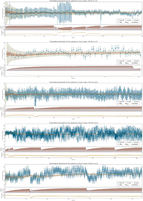
www.nature.com/scientificreports/
Figure 1. The schematic diagram of the experimental setup. All optics and detectors are placed inside the
vacuum chamber. The electronic equipment and the laser are kept outside.
Figure 2. A picture of optics in the open chamber.
DFB-1368-A-A81-SA) operating at ∼ 1368.60 nm with 2 MHz line width is used to scan 101313–00021211 water
absorption line. The DFB CW output power is about 1 mW at 27 ◦C. The laser diode is equipped with an internal
InGaAs photodiode. The DFB diode is controlled by an integrated current and temperature controller (Thorlabs,
CLD1015) placed outside the chamber. The temperature setting of the diode is set to 27 ◦C. The laser beam is fed
into the chamber using single-mode optical fibers (SMF-28E and SMG652.D) using vacuum feedthrough (SQS,
KF40 SM). The beam is collimated with adjustable ECO-550 lenses (Thorlabs, PAF2-2C). The vertical multi-pass
setup is made up of two 3” dielectric concave mirrors f = 500 mm (Thorlabs, CM750-500-E04-SP) held vertically
by metal rods about 76.7 cm apart from each other. Two flat silver mirrors (Thorlabs, MRA03-P01, MRA10-
P01) are used to direct laser beam from the collimator to/from the multipass cell and towards a 92/8 pellicle
beamsplitter (Thorlabs, CM1-BP108). The first flat mirror that directs the laser beam up to the multipass cell is
approx. 8 cm from the collimator. The beamsplitter is approx. 20 cm away from this mirror. Detector 1 is approx.
5.2 cm from the beamsplitter, Detector 2 is 6.7 cm away. The total light path length is approx. 61.4 m long and it
is ∼ 1.5 cm shorter towards Detector 1. The multipass cell axis is in line with the chamber vertical axis to assure
equally long distance from the chamber walls, approx. 25 cm. All optical components are installed on a small
breadboard standing on the chamber floor, see Fig. 2.
Transmittance is measured in parallel by a pair of ø200 µm InGaAs photodiodes (Hamamatsu G11193-02R).
A circular aperture stop to reduce detector’s effective active area is inserted in front of the detector (Ch1) placed
in line with the beamsplitter incoming beam, see Table 1. The aperture is installed ∼ 1 mm away from the pho-
tosensitive surface. The second detector (Ch2 ), without an aperture, gives a reference transmittance reading.
Both detectors and the aperture stop are installed in their own X–Y translation units. The ∼ 92% of the beam
is directed towards the first detector.
Both photodiodes operate in a photovoltaic m ode12 with no bias voltage. The photodiode current is a mplified13
by a custom-built current-to-voltage amplifier using the low current op-amp (TI, LMC662), followed by a
Scientific Reports | (2021) 11:6221 | https://doi.org/10.1038/s41598-021-85568-w 2
Vol:.(1234567890)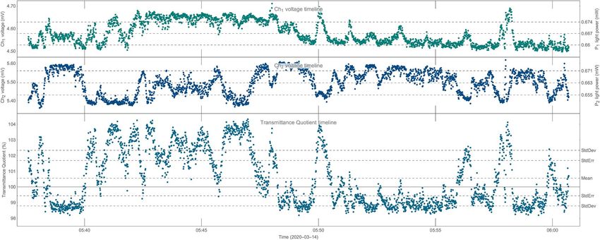
www.nature.com/scientificreports/
Size 2 µm 5 µm 15 µm 25 µm 40 µm 50 µm 100 µm 150 µm
Model P2H P5D P15D P25D P40D P50D P100D P150D
Diameter tolerance ±0.25 µm ±1 µm ±1.5 µm ±2 µm ±3 µm ±3 µm ±4 µm ±6 µm
Circularity ≥85% ≥90% ≥90% ≥95% ≥95% ≥95% ≥95% ≥95%
Gain - resistor ( ) 50 × 106 10 × 106 51 × 103 51 × 103 51 × 103 51 × 103 2 × 10³ 2 × 10³
Table 1. Ch1 aperture stops parameters.
Run name R-3 R-5 R-6 R-7 R-8 R-9 R-10 R-11 R-12 R-13 R-14 R-15
Aperture installed 2 µm 2 µm 25 µm 5 µm none 150 µm none 15 µm 40 µm 25 µm 50 µm 100 µm
No. of cycles 131 218 71 81 31 268 709 558 645 1177 1014 1012
No. of measurements 384 289 577 676 183 212 214 318 80 220 695 544 1 185 491 262 717 202 953 555 846 478 307 479 172
Table 2. Basic statistics of the experiment runs.
low-pass 10 Hz RC filter. The amplifier gain is controlled by a feedback loop resistor. The Ch1 resistance is adjusted
for each aperture individually to keep output voltage within a range of a few dozen mV, see Table 1. The Ch2
resistance is constant and equal to 2k . Gains are chosen to obtain both characteristics curves as linear as pos-
sible within the range used for actual measurement.
Vacuum is evacuated with a scroll pump and a turbo molecular pump. Two independent vacuum meters are
used (Leybold, Ceravac CTR 100N, Ionivac ITR90).
All voltage data is acquired by the DAQ unit (LabJack, U6). The digital data, from the DAQ unit and the
laser driver, is retrieved via a USB by a PC computer running LabView. A custom built LabView GUI is used to
automate the measurement procedure. The LabView text files data is extracted periodically into the SQL database
from where it is retrieved for statistical analyses performed by the Mathematica 12 package.
In this paper Ch1 and Ch2 may denote either a respective photodiode or one of measurement channels or a
voltage read from one of channels.
Gas and spectral line selection. We selected water vapor due to its large cross-section in the near infra-
red. The HITRAN14 and MARVEL15 data was referenced. The large cross-section allows for testing transmittance
at low pressures with shorter path of light. Low pressure and a narrow spectral range of the laser allow for isolat-
ing a single absorption line with sufficient resolution.
For our setup the expected mean free path of water particles for the pressure of ∼ 10−3 mbar is longer than
37 cm. With approximate mean speed in the room temperature of 600 ms−1 it gives approx. 0.6 ms particle mean
free time. Plugging this time to the Schrödinger equation free particle solution we calculate the particle wave
packet standard deviation to be ∼ 14.6 µm. This is a conservative calculation using ideal gas laws.
The chamber size is another restriction on the particle mean free path. There should be enough distance
between walls and the measuring laser beam. This is why a chamber diameter of 58 cm was chosen.
Stages of the experiment. The experiment is carried out in successive, several days long runs, see Table 2.
There is a different aperture stop installed during each run. A run consists of many consecutive either ∼ 30 min
or ∼ 10 min long cycles.
Replacement of an aperture requires opening of the vacuum chamber. After the aperture installation, the Ch1
gain is adjusted by soldering in the appropriate feedback loop resistor. In case of two runs (R-8 and R-10), the
aperture stop was removed in order to perform a comparative measurement for two detectors equal (according
to manufacturer) in size.
After the chamber has been closed, vacuum is build to ∼ 10−5 mbar , which takes roughly 1–2 days. In some
cases, the decision was taken to extend this period to 3–5 days. Water is sucked in from an external tank due to
the pressure difference. Dosing is controlled using a needle valve adjusted by a manual micrometer screw. Water
vapor is produced as a result of spontaneous boiling of water at low pressure.
Water vapor tends to settle on the inside walls of the chamber and setup components16. This can be seen in
the spontaneous pressure drop, starting immediately after the feed valve has been closed. To obtain the working
pressure in the order of 10−3 − 10−2 mbar , the valve is kept open for a longer period of time (e.g., an hour),
while maintaining higher pressure (e.g., 2 × 10⁻² mbar ), see pressure plots in Fig. 9.
The pressure measurement below 10−3 mbar, made using the Ionivac vacuum gauge (PRSB), is burdened with
quite a large error, in the order of ±15%. However, this range is used solely to build vacuum prior to feeding
the water. The total working pressure, i.e. above 10−3 mbar , is measured, with the accuracy of ±0.5%, using the
Ceravac vacuum gauge ( PRSA). The partial pressure of the water ( PRSH2 O ) may be determined by converting
the classical transmittance measured with Ch2, see Eq. 6. The partial pressure can be determined in our setup
within the range of approx. 1 × 10⁻³ − 3 × 10⁻² mbar.
To purify the chamber atmosphere vacuum may be build and water may be fed many times during a single
run without opening the chamber. These operations are visible as discontinuities on pressure plots in Fig. 9.
Scientific Reports | (2021) 11:6221 | https://doi.org/10.1038/s41598-021-85568-w 3
Vol.:(0123456789)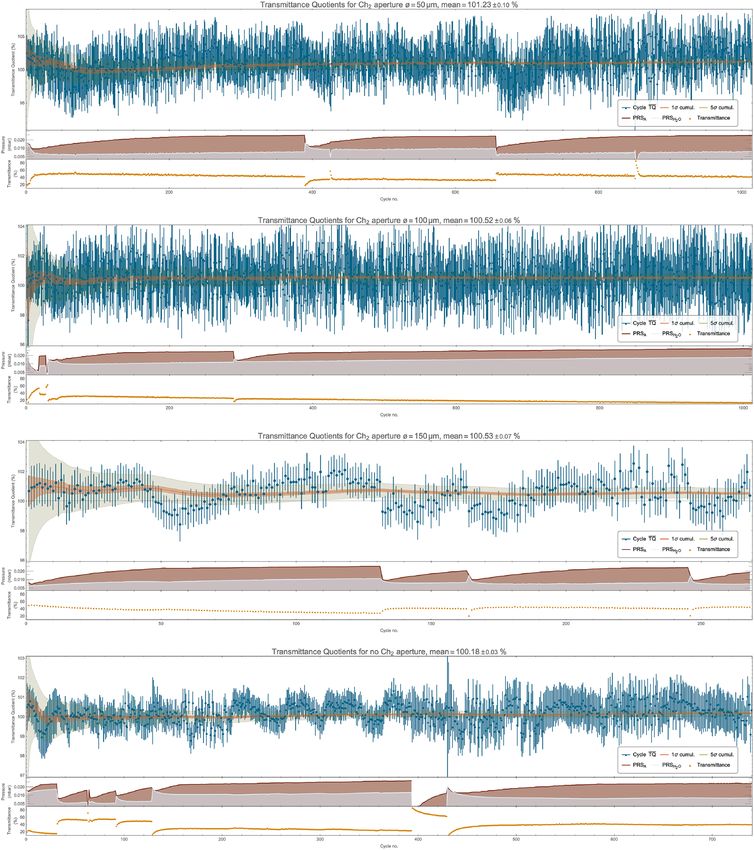
www.nature.com/scientificreports/
Figure 3. Sample readings of the Ch2 detector during two successive 30 min cycles along with both cycles steps
numbers are presented. Reversing laser current step is visible at the 1st step of the second cycle.
Data acquisition
Within a single run the measurement is made in cycles composed of following steps:
1. measuring detectors characteristic curves,
2. tuning in the wavelength of the laser light to the chosen absorption line,
3. measuring both transmittances,
4. measuring detectors characteristic curves again (with the laser current step reversed).
The 4th step is the 1st step of the next cycle. Fig. 3 presents sample readings of the Ch2 detector during two
successive cycles. Cycles last either 30 min or (in the 2nd part of the experiment) 10 min. All cyclic measurements
are fully automated with a LabView app. Each cycle has its own, time-based identifier assigned e.g., 20200314-
0531. The identifier is referred during data post processing and data presentation.
Detector characteristics acquisition (step 1). The setup is susceptible to various types of drifts: laser
tuning, changes in light polarization in optical fibers (affecting the detector readings), pressure and mechanical
changes. They cause, among others, a change of the detector characteristics. Due to the adopted method of deter-
mining the transmittance quotient, acquiring the appropriate voltage versus light power characteristic curves is
of key importance: P1 (Ch1 ) and P2 (Ch2 ). Although they are called for convenience “detectors characteristics”,
they are not just photodiodes characteristics. They cover all light & signal processing steps in turn: the fibers &
mirrors light attenuation, the aperture stop (Ch2 only), the photodiodes light-to-current conversion, the current-
to-voltage conversion & amplification and A/D conversion.
The characteristics are determined by changing the DFB diode current ILD . Based on the fact that the DFB
diode output power is proportional to the current set, the detector response is determined as a function of the
laser power. The range of current changes is automatically selected based on the last reading (from the previous
cycle) of the transmittance in the absorption line. It is assumed that the transmittance in the current cycle will
be similar to the previous one, i.e. that the partial pressure of the water vapor does not change significantly.
The span of the ILD current changes is arbitrarily set as either ILD = ± 12 mA for 30 min long cycles or
ILD = ± 9 mA for the shorter ones. DFB controller’s minimum current step is 0.05 mA . It is known that a
change of the DFB diode current also causes a change of the wavelength. In case of the diode used in the
experiment � /�ILD ≈ 78 pm mA−1, which for (current span of) 24 mA leads to a change of the wavelength
by ∼ 1.8 nm. We chosen span and range to avoid overlapping with other strong absorption lines while charac-
teristics acquisition.
Such a change in wavelength may also cause a slight change in detector sensitivity (up to 1% according to
the manufacturer). It is assumed, however, that due to the use of two detectors from the same series, the relative
change in sensitivity between the detectors is the same. The same offset cancels possible measurement error
because it appears both in the numerator and the denominator of the formula used to determine the transmit-
tance quotient, see Eq. (3).
It is required that the actual laser temperature is within the ±0.003% range from the set point of 27 ◦ C for each
measurement. The scan starts 250 ms after reaching required temperature range. Each recorded measurement
within a scan is the arithmetic mean of 30 consecutive single readings (Ch1, Ch2, PLD ) made every 11 ms. Despite
allowing a fairly narrow range of stabilized temperature, the current change direction (up/down) is switched in
each cycle. It’s either +0.05 mA or −0.05 mA. A constant increase (or a decrease, accordingly) of the laser current
ILD makes the laser diode working temperature always a little higher (or lower, accordingly) on average. This is
because the temperature compensation circuit (Peltier TEC, PID) keeps up with the current changes quite slowly.
To compensate this effect the measurements obtained both at the beginning and at the end of the cycle (steps 1 &
4) are used together to calculate the characteristic curve for the given cycle. This way up to 2×2×12/0.05 = 960
(or later 2×2×9/0.05 = 720) points are available for approximate characteristics models.
The scan range may be automatically limited from the bottom. For higher pressures (in the order of
10−2 mbar ) the absorption line is so deep that only a few percent of the light reaches the detectors. In such case
the characteristic is obtained close to the lower limit of the laser action and it is impossible to measure some of
the distant points in the ILD negative range. The measurement of the characteristics is then limited so that the
ILD current fed is large enough (min. 3 mA ) to excite the laser action.
Scientific Reports | (2021) 11:6221 | https://doi.org/10.1038/s41598-021-85568-w 4
Vol:.(1234567890)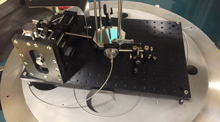
www.nature.com/scientificreports/

                                  Figure 4.  Example of linear approximation of both characteristics along with source measurements. The
                                  colored vertical stripe indicates the range of the detected voltage variability in the cycle. The grey vertical stripes
                                  indicate an additional range (up to 25%) of the points used to determine the linear regression.

                                     The scan range is limited from the top as well. Laser current ILD can’t exceed 52 mA , so that, by accident, no
                                  measurement of the water absorption line is made.
                                     The characteristic acquisition takes approx. 6 minutes. Most of this time is spent waiting for temperature
                                  stabilization of the laser.

                                  Tuning in the wavelength (step 2). After the characteristics has been measured, a fixed value of the laser
                                  current ILD is set to get the wavelength as close as possible to the absorption line maximum. Because of drifts of
                                  the diode and the controller it’s necessary to adjust the laser current ILD . We check, for 3 distinct settings, which
                                  transmittance in the Ch2 detector is the lowest: one that is identical as in the previous cycle or one that is different
                                  by either plus or minus 0.05 mA. Checking starts 45 seconds after the measurements of the characteristics had
                                  been completed, providing time to properly relax temperature of the laser to the range of ±0.003%. This way,
                                  actual wavelength is kept as close as possible to the absorption maximum during the entire experiment.

                                  The transmittances measurement (step 3). Having set the fixed laser current and temperature set-
                                  points near the absorption line maximum, the transmittances measurement is carried out in the continuous
                                  mode. We don’t use any wavelength modulation techniques. Single measurements are recorded twice a second.
                                  A single measurement includes following parameters read synchronously: both detectors voltages (Ch1, Ch2),
                                  laser power read from the laser photodiode ( PLD ), actual laser temperature and current (TLD , ILD ) as well as both
                                  pressure readings ( PRSA, PRSB). This measurement step ends half an hour (or 10 min) from the start of the cycle.

                                  The 2nd characteristics acquisition (step 4). The last step in the cycle is to acquire measurements for
                                  the characteristics again. This time, stepping the laser current in the reverse direction. It is also the first step of
                                  the next cycle.

                                  Data processing
                                  The difference of the water vapor transmittances measured by both detectors is calculated as the transmittance
                                  quotient (TQ) according to the following procedure.

                                  Determination of the linear model of the detector characteristics. The characteristics P1 (Ch1 )
                                  and P2 (Ch2 ) of both detectors are determined for each measurement cycle. They are approximated with a linear
                                  regression near the range of the detector voltage values observed during the given measurement cycle:
                                                                                 P1 (Ch1 ) =A1 Ch1 + B1 ,
                                                                                                                                                      (1)
                                                                                 P2 (Ch2 ) =A2 Ch2 + B2 ,
                                  where A1,2 and B1,2 are linear model coefficients.
                                       There are up to 960 (or 720) points (Ch1n, PLDn), (Ch2n, PLDn) available for each linear regression fitting. PLD is
                                  the power of light emitted by the laser as reported by the DFB built-in photodiode, Ch1,2 is the detector’s voltage
                                  reading, the n index denotes the subsequent readings during scans. See Fig. 4.
                                       A set of points used for actual fitting is limited to the range of voltages measured by the detector within the
                                  cycle. It gives linear approximation with a smaller error within the interesting range. Usually these are very
                                  narrow ranges of detector operation (e.g. tenths of mV ), resulting from noise and a small pressure difference
                                  during the cycle. Very often they are so narrow that there are too few measurements available for accurate model
                                  fitting. The range is then extended up to 25% of the voltage range of the characteristic being measured. This way
                                  the model is fitted using approx. 150–200 points only. Thanks to the surplus of points, the linear regression can
                                  be assessed visually in a broader context, see overview in Fig. 4. Such plots are available online for all measure-
                                  ment cycles.

Scientific Reports |   (2021) 11:6221 |                 https://doi.org/10.1038/s41598-021-85568-w                                                      5

                                                                                                                                                   Vol.:(0123456789)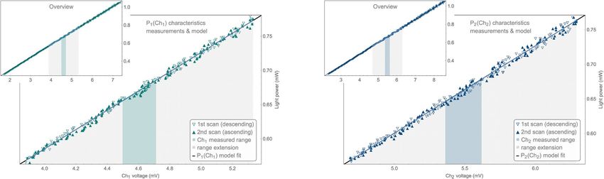
www.nature.com/scientificreports/

                                            Figure 5.  Example of the linear regression residuals—only within the range of points designated for
                                            determining the regression.

                                                The quality of the approximation is assessed for each cycle by independently using parameter R2 . The
                                            residuals graph may be also examined, see Fig. 5. Usually cycles where pressure fluctuations are too large (i.e.
                                            Max(PRSB ) − Min(PRSB ) > 5 × 10⁻³ mbar ) are skipped because there is no way to find a good enough linear
                                            approximation. Most often these are the first 1-2 cycles after feeding water into the chamber.
                                                The measurements obtained at both ends of the given cycle are used together to determine the detectors
                                            characteristics models. They always differ based on the direction of the laser current change (“up” or “down”).
                                            This way, any potential systematic shifts of the characteristics related to the laser temperature relaxation is elimi-
                                            nated. The triangles direction in Figs. 4 and 5 denote measurements from two different directions of obtaining
                                            the characteristics.
                                                We chose the parameters of the experiment (i.e. temperature and range of the laser current, absorption line,
                                            working pressure and length of the light path) in the way the characteristics are determined in a range where
                                            other water absorption lines are sufficiently weak. Therefore, water vapor do not cause any disturbances of the
                                            detector characteristics model calculations.

                                            Transmittance Quotient calculation. Gas optical transmittance is the ratio of the power of the light
                                            beam that has passed through the medium divided by the power of the light that has entered the medium. The
                                            characteristics of the detectors calculated above allow for calculating the transmittance for each of the channels:
                                                                                           TR1 =P1 (Ch1 )/PLD ,
                                                                                                                                                              (2)
                                                                                           TR2 =P2 (Ch2 )/PLD .
                                                All “constant” light power loses for both measurement channels are encoded within P1 and P2 models, respec-
                                            tively. These loses mainly result from mirrors reflectivity, photodiodes efficiency and beam splitting. This way
                                            the Eq. (2) are valid for determining just water vapor transmittance.
                                                We compare transmittance values using the transmittance quotient (TQ) as defined below:
                                                                                       TR1   P1 (Ch1 )/PLD   P1 (Ch1 )
                                                                                TQ =       =               =           .                                      (3)
                                                                                       TR2   P2 (Ch2 )/PLD   P2 (Ch2 )
                                                Note that the quotient defined above is not a simple quotient of light power measured by both detectors. It
                                            is the quotient of transmittances measured by both detectors.
                                                There is either transmittance difference or transmittance quotient referred in this report. Transmittance
                                            difference is expressed as a percentage so it is just the transmittance quotient minus 1. TQ values greater than 1
                                            (transmittance difference greater than 0) mean that the transmittance measured by the smaller detector Ch1 is
                                            greater than the transmittance measured by the classical one Ch2. Examples of the TQ values for the individual
                                            measurements are shown in Fig. 6.
                                                There is a possible issue with a non linearity of the DFB laser diode (current vs output power) and the DFB
                                            photodiode (incident light vs current). It was checked that this non linearity is so small in the operational range
                                            that it doesn’t significantly affect transmittance measurement. It should be taken into account for very accurate
                                            transmittance measurements. Besides we’re interested just in transmittance quotient in this experiment. This
                                            non linearity cancels out because it appears in both numerator and denominator of Eq. (3).
                                                The actual reading (including its error) of the laser photodiode ( PLD ) is irrelevant for the calculation of
                                            transmittance quotient TQ because it cancels out appearing in both numerator and denominator of Eq. (3).
                                                Determination of the transmittances and their quotient is possible only if the domains of characteristics P1,2
                                            includes the appropriate range of the Ch1,2 voltages. It is checked automatically for each cycle. If the appropriate
                                            characteristic range is missing the measurements made within the given cycle are skipped by the aggregating
                                            algorithm. It may happen sometimes for sudden pressure changes.
                                                There is a small (∼ 1.5 cm) difference in total light path length towards detectors. Because light path towards
                                            Detector 1 is ∼ 0.024% shorter transmittance measured by Detector 1 is systematically ∼ 0.024% higher. We will
                                            see later that such a difference is negligible but it should be noted.

                                            Transmittance Quotient aggregation. We determine the transmittance quotient for each single meas-
                                            urement within a cycle. There are 2 measurements per second recorded which makes hundreds measurements
                                            per cycle. Assuming that the experimental conditions are sufficiently constant during the cycle, the average
                                            transmittance quotient TQk for the entire cycle is determined:

          Scientific Reports |   (2021) 11:6221 |                https://doi.org/10.1038/s41598-021-85568-w                                                     6

Vol:.(1234567890)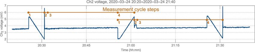
www.nature.com/scientificreports/
Figure 6. Example of the Ch1, Ch2 and transmittance quotient (TQ) measurements within a single cycle.
Mk
1 P1k (Ch1m )
TQk =
Mk P2k (Ch2m )
m=1
Mk
(4)
1 A1k Ch1m + B1k
=
Mk A2k Ch2m + B2k
m=1
where k-cycle index, Mk-number of the single measurements in the k-th cycle, m-measurement index within a
cycle, A1,2k , B1,2k-linear regression factors of P1,2k characteristics, respectively for channel 1 and 2.
Determination of the transmittance quotient TQ for the entire run (for single aperture) involves calculating
the arithmetic mean of the quotients measured in the successive cycles:
K
1
TQ = TQk (5)
K
k=1
where K-number of cycles in a run.
Water vapor partial pressure calculation. Having determined the classical transmittance in the Ch2
channel, the partial pressure of water vapor ( PRSH2 O ) can be determined based on the relationship between
transmittance, absorbance and pressure:
PRSH2 O ≈ −0.00854 Log(TR2 ) mbar . (6)
We calculated the conversion factor depending on light path length, absorption line cross-section and
temperature.
Results and interpretation
The aggregated results of the experiment are presented in Fig. 7. The mean transmittance quotient TQ is shown
for each individual aperture examined. The rightmost point is the result of no aperture runs. All measured values
are greater than 100%. It means that the Ch1 (smaller) detector measured higher transmittance.
All presented quantitative results (transmittance quotient and transmittance difference) don’t take into
account the systematic shift introduced by the ∼ 0.024% shorter light path towards Detector 1. This is because
one may simply shift the reference base from 100% to 100.024% when analyzing if transmittance measured with
the smaller detector is greater or not.
The more detailed graphs showing the values of measurements for the individual cycles along with pressure
and transmittance are presented in the Appendix, see Fig. 9. Yet more data and figures are available online at
www.smearedgas.org/experiment1. Among others, there are “cycle cards” prepared for all measurement cycles.
They presents all essential data collected during single cycle along with parameters calculated, see Appendix for
the guide. Raw data is available upon request.
Runs with aperture stops. We observe that all runs with the pinhole installed show higher transmittance
when measured by the smaller Ch1 detector! This is exactly the effect qualitatively predicted by the smeared gas
theory. For runs with bigger, namely 25-, 40-, 50-, 100- and 150 µm apertures, the statistical significance is higher
than 5σ.
Scientific Reports | (2021) 11:6221 | https://doi.org/10.1038/s41598-021-85568-w 7
Vol.:(0123456789)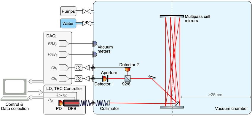
www.nature.com/scientificreports/
Figure 7. The aggregated results of the experiment: mean transmittance quotients TQ along with their 1σ
standard errors (vertical bars) and aperture tolerances (horizontal bars). The transmittance quotients are
averaged for all pressures for each examined aperture. The rightmost point is the result of no aperture runs.
Quotient greater than 100% means that transmittance measured by the smaller (< 200 µm) Ch1 detector is
higher than transmittance measured by the bigger (200 µm) Ch2 detector, which is the case for each run.
The maximum transmittance difference equals to 1.23 ± 0.1 %, when the 50 µm aperture is installed. For
the 100- and 150 µm apertures the difference is equal to 0.52 ± 0.06 % and 0.53 ± 0.07 % respectively. They are
smaller than the 50 µm aperture result. This is in line with the model’s qualitative prediction: as the detector size
increases, the measured transmittance should decrease—for detectors significantly larger then the wavelength
(a kind of geometric optics approximation).
This relationship is the other way around for the 6 smallest apertures, however. Furthermore, for the 3 small-
est apertures the statistical significance falls down to 2–3σ . This is because the transmittance, according to the
smeared gas model, is proportional to the definite integral of | |2 over so-called “visibility tunnel”. The visibility
tunnel is a volume where a photon amplitude doesn’t cancel out when using certain detector - according to
the path integrals a pproach17. For detectors comparable in size to the wavelength the non-cancelling photon
probability amplitudes outside the “classic” visibility tunnel effectively thicken this tunnel. This increases the
volume over which the probability distributions of the smeared gas particles are integrated. As a consequence,
the likelihood of observing a photon scattering event with such a small detector rises. Therefore, the measured
transmittance decreases—in the extreme case down to the classical transmittance level. We see this kind of rela-
tion on the left side of the Fig. 7. The transmittance quotient is decreasing towards 100% along with decreasing
Ch1 detector aperture diameter (from 50- down to 2 µm).
The result for the 100 µm aperture (with much higher average pressure) is discussed later on. The very low
reading for the 15 µm aperture needs further analysis.
The quantitative model fitting to experimental results will be performed further down the line. Still, we
observe qualitative predictions are met in the experiment.
Control runs without aperture. During the R-8 and R-10 runs there are no apertures installed. Transmit-
tance is measured using two naked detectors with a comparable diameter. The measured transmittance differ-
ence is 0.12 ± 0.04 %. The transmittances are thus not perfectly identical but very close to each other.
Apart from obvious measurement errors, such difference may result, for example, from the diameter toler-
ance due to the workmanship of the detectors themselves, impurities etc. This tolerance, in turn, is irrelevant in
case of the measurements made with aperture stops in place because detector Ch1 is obscured by the aperture
anyway. Another reason for the observed difference may be a potential variance in the sensitivity of both detec-
tors to different wavelengths as discussed earlier. This may cause some systematic error when determining the
characteristics of all measurements. However, this control runs would indicate at least the order of magnitude
of such a systematic error. Even if it is ∼0.12 %, it is still significantly smaller than the measured transmittance
differences for 5 apertures larger than 25 µm. Consequently, it does not undermine the conclusions drawn.
Transmittance quotient versus pressure. There are at least two phenomena influencing the transmit-
tance quotient that should be taken into account when the pressure changes and temperature is kept constant. As
the pressure increases, (1) the number of molecules increases (the transmittance drops), (2) the mean free path
shortens. The experiment was not designed to examine these correlations so very little may be concluded in this
field. However, there are some indications we can take a closer look at. They are in accordance with the model.
Transmittance quotient versus number of molecules. According to the model the increasing num-
ber of molecules with the mean wave function spread unchanged (aka the mean free time constant) along with
a fixed visibility tunnel should increase the transmittance quotient. We show it qualitatively on the Fig. 8. There
are presented sample predictions of the model in a range of “geometric optics” approximation for two different
water vapor partial pressures: ∼ 1 × 10⁻² mbar and ∼ 6 × 10⁻³ mbar . According to Eq. (6) they correspond to
Scientific Reports | (2021) 11:6221 | https://doi.org/10.1038/s41598-021-85568-w 8
Vol:.(1234567890)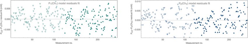
www.nature.com/scientificreports/
Figure 8. A comparison of the experiment results with exemplary predictions of the model taking into account
the basic pressure dependence. Solid lines represent exemplary predictions of the model in a range of “geometric
optics” approximation (see text) for two different pressures (expressed as 30% and 50% transmittances). The
measured transmittance quotients TQ averaged for two distinct TR2 transmittances ranges (20–40% and 40–60%
respectively) are presented with 1σ standard error bars. The 5-, 15- and 100 µm apertures are omitted due to
missing data in this range of pressures. The transmittance quotients averaged for all pressures for all apertures
are superimposed for convenience (blue circles without error bars).
transmittance (TR2) of 30% and 50% respectively. The transmittances for each detector d = 1, 2 are calculated
with the following equation9:
N
2
Gd () on − rTd on + rTd
TRd (t̄) = 1− erf √ − erf √ , (7)
4 2stdevAn (t̄) 2stdevAn (t̄)
n=1
where t̄ denotes the molecules mean free time, N is a number of molecules in the chamber, on is the n-th mol-
ecule distance from the beam. The standard deviation stdevAn (t̄) is assumed to be ∼ 14.6 µm (see next para-
graphs). The geometry coefficient Gd () is equal to cross section of the 101313-00021211 water absorption line
(≈ 7.76 × 10⁻¹⁹ cm2 ) divided by the area of the detector. Theoretical transmittance quotients are calculated
assuming the transmittance tunnel has the shape of a 60 m long truncated cone. The smaller base is of the size of
an aperture. The angle (an effective divergence towards the source) is 0.008 mrad . Note, that this divergence is
much smaller than the typical laser beam divergence thanks to the spherical mirrors re-focusing the beam for 80
times. The rTd is the radius of the (cylindrical) visibility tunnel, it’s different for each detector d. For simplifying
calculations the conical tunnel is approximated as a cylinder, thus rTd is equal to the mean of both bases radii.
There are TQ measurements shown on the Fig. 8 for at least 4 different apertures: 25-, 40-, 50- and 150 µm
following the model qualitative prediction: TQ is higher for the higher pressure. The statistical significance of this
relation reaches as much as 3σ for the 25- and 40 µm apertures. Measurements for other apertures and pressures
are omitted due to missing comparable data.
Transmittance quotient versus mean free path. The measured transmittance quotient for the 100 µm
aperture stop is smaller than ones measured for 50- and 150 µm apertures, see Fig. 7. According to the model
TQ closer to 100% may indicate a shorter mean free time. Indeed for the 100 µm aperture stop, most of the time
the total pressure was higher than 3 × 10⁻² mbar and the water vapor partial pressure PRSH2 O was higher than
1 × 10⁻² mbar . The measurements for other apertures was made at a lower total pressure, approx. in a range
from 1 × 10⁻³ mbar to 3 × 10⁻² mbar . It seems that so high pressure eventually led to shortening the mean free
path to a value smaller than the one constrained by the chamber size. This way the water molecule wave function
standard deviation might drop below 14.6 µm lowering the TQ reading.
Further works
First of all it is necessary to conduct the quantitative model fitting. Careful consideration of the shape of the
visibility tunnel is essential. All factors like reflections, collimation, laser power density or small apertures (non-
classic trajectories) should be taken into account.
The experiment should be repeated under modified conditions to eliminate any missed systematic errors and
increase accuracy. Potential modifications include, among others:
• making both light paths equal in length,
• analyzing and/or avoiding interference caused by the single mode laser (fringes),
• a split of the beam in parallel towards more than 2 detectors,
• mounting apertures at each detector and testing the differences under varying configurations of reflection
and beam split, e.g., 50/50 split,
Scientific Reports | (2021) 11:6221 | https://doi.org/10.1038/s41598-021-85568-w 9
Vol.:(0123456789)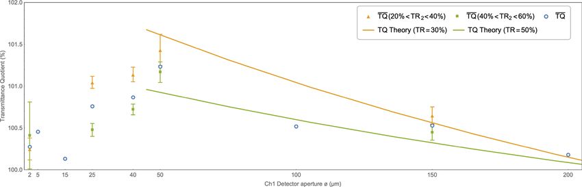
www.nature.com/scientificreports/
• better ways to reduce diode noise, e.g., changing the wiring or moving the first stage amplifiers closer to
photodiodes, even inside the vacuum chamber,
• more precise tuning of the wavelength to the absorption line using externally modulated laser driver, con-
trolled with the standalone wavemeter or the lock-in feedback l oop18,
• increasing the diameter of the vacuum chamber (extending the mean free path),
• more stable fastening of the multi-pass cell mirrors,
• removing the multi-pass cell rods shortening the mean free path near the laser beam,
• applying a different number of reflections in the multi-pass cell,
• assembling the measuring system outside the main section of the vacuum chamber so that the system could
be reconfigured faster,
• testing other gases e.g., methane (also with a large cross section in NIR).
A slight modification of the proposed method will allow for conducting measurements of transmittance differ-
ences and mean free paths for larger working pressure ranges. In particular, the length of the light path should
be adjusted by controlling the number of reflections in the multi-pass cell. The experiment can be carried out
without the use of a multi-pass cell, using a sufficiently long vacuum chamber.
Another modification may involve enabling limiting and adjusting the mean free path by installing internal
walls or pipes. This will allow for studying the relationship between the transmittance quotient and the mean
free path.
The presented values of the transmittance quotient in a range of 1% may not seem respectable. However,
higher values can be achieved e.g., by lengthen particles mean free time in a bigger chamber.
Conclusions
For ultra thin gas we observed the effect of changing the optical transmittance measurement readings using
detectors of different sizes. For detectors of a diameter much bigger than the wavelength transmittance increased
as detector size decreased. Thus, the objective of the experiment, which is to observe in laboratory conditions the
qualitative effect predicted by the non-local smeared gas transmittance m odel9, is achieved. The fact of observing
a non-obvious phenomenon predicted by the theory is a strong premise for its validity. As far as we know there
is no other gas transmittance model predicting such results.
The results are presented with a very high statistical significance level thanks to the long, repetitive measure-
ment process. However, too few measurements were made to categorically determine the type of relationship
between transmittance quotient and pressure. Moreover, there are many other improvements available regarding
robustness, accuracy, flexibility etc. Some of them are outlined in the paper.
This experiment is a kind of a typical quantitative spectroscopy setup. It is relatively cheap and easy to repeat.
However, it differs in two very important details from a well known TDLAS. Firstly, a sufficiently long gas par-
ticles mean free path is required. Free from any reactions that could be considered a quantum measurement or
lead to decoherence. Therefore, the following should be provided: a large chamber, low pressure, electromagnetic
shielding and weak measurement laser light. Secondly, the detector’s light sensitive diameter should be com-
parable (or lower) to the standard deviation of the smearing of the tested gas particles wave packets. It seems
highly unlikely that both of these conditions could have been accidentally met during some earlier quantitative
spectroscopy experiment. No reports of a similar experiment have been found in the literature.
In the experiment quite small detectors where used and a moderate pressure with a not so long light path
was examined. However, the shown predictions of the smeared gas model apply for lower pressure levels, bigger
detectors and longer distances. We believe the suitability of the smeared g as9 model should be verified in relation
to the conditions of astronomical measurements.
Appendix
Cycle measurement results. There are measurement results for each cycle presented in Fig. 9. They are
grouped by the Ch2 aperture size, aggregating data from different runs if required. Each point on a plot repre-
sents the measurement result for an entire (either 10- or 30-minutes long) cycle. The graphs also present bands
showing the 1σ and 5σ measurement uncertainties accumulated for the preceding cycles. There are both total &
partial pressure and transmittance plots superimposed. Single measurements results are available online.
Online data. Online data & additional material are available on the website https: //www.smeare dgas. org/exper
iment1. There is a separate web page for each aperture size available. It consists of a run (or runs) summary,
timeline figures and a list of measurement cycles within those runs. For each cycle on the list there is a link to a
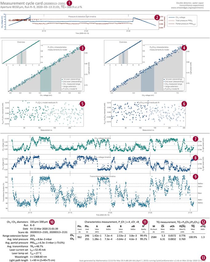
“cycle card”. All single measurements taken during a cycle are shown on a single cycle card. A sample cycle card
is presented in Fig. 10. It consists of the following sections.
1. The title of the card includes id of the cycle, the aperture diameter, the run name, timestamp the cycle
started and the mean transmittance quotient (TQ) as measured in the cycle.
2. The timeline of the cycle contains the total & partial pressures (red, dashed) and power of light (blue)
as detected by the reference (Ch2) detector. The partial pressure is calculated only for the period during
which the transmittance measurement was carried out (the 3rd step of a cycle). The total pressure shown
is measured with the PRSA vacuum meter.
3. The linear approximation of the Ch1 characteristic along with source measurements. The colored vertical
stripe indicates the range of the detected Ch1 voltage variability during the cycle. The grey vertical stripes
indicate an additional range (up to 25%) of the points used to determine the regression. The triangle direc-
Scientific Reports | (2021) 11:6221 | https://doi.org/10.1038/s41598-021-85568-w 10
Vol:.(1234567890)www.nature.com/scientificreports/
Figure 9. Mean transmittance quotients along with their 1σ standard errors for the individual cycles and
the bands showing the accumulated 1σ and 5σ measurement uncertainties, both total & partial pressures and
transmittance readings are superimposed.
Scientific Reports | (2021) 11:6221 | https://doi.org/10.1038/s41598-021-85568-w 11
Vol.:(0123456789)www.nature.com/scientificreports/
Figure 9. (continued)
tion reflects the laser current stepping direction during scanning (the 1st & 4th steps of a cycle). Refer to
Fig. 4 notes in the main text for more details.
4. The same as the #3 above but for the Ch2 detector.
5. The Ch1 linear regression residuals - within the range of points designated for determining the regression.
6. The same as the #5 above but for the Ch2 detector.
7. The timeline contains each single reading of the Ch1 detector recorded. The left axis presents raw voltage
as reported by the DAQ unit. On the right axis there is the corresponding power of light as calculated with
the current cycle’s P1 characteristic model. The dashed horizontal lines denote the mean value and ±1σ
deviation.
8. The same as the #7 above but for the Ch2 detector.
9. Each point is the transmittance quotient TQm calculated for a pair of Ch1m & Ch2m values from the same
measurement. The dashed horizontal lines denote the mean value, its standard deviation and the standard
error of the entire cycle.
10. A variety of the run and cycle parameters.
11. The parameters of both P1 & P2 characteristics models determined in the cycle.
Scientific Reports | (2021) 11:6221 | https://doi.org/10.1038/s41598-021-85568-w 12
Vol:.(1234567890)www.nature.com/scientificreports/
Figure 10. All measurements taken during the cycle are shown on a sample cycle card. The numbers in the
circles refer to the sections descriptions in the text.
Scientific Reports | (2021) 11:6221 | https://doi.org/10.1038/s41598-021-85568-w 13
Vol.:(0123456789)www.nature.com/scientificreports/
12. The mean transmittance quotient for the cycle (referred as TQk in the main text) along with its standard
error and other uncertainty related parameters: the number of measurements, the mean detector readings
and the relevant standard deviations.
13. The footer contains the software version used & card generation timestamp.
Uncertainty and errors. Two main areas where errors originate can be distinguished in the system: i)
errors in determining the characteristics of the detectors and ii) errors while performing the actual measurement
of the transmittance i.e., power of light received by the detectors. The error in determining the characteristic is a
systematic error in measuring the transmittance quotient in the given cycle. When aggregating data from multi-
ple cycles, this error becomes a random error, however. Therefore, the rules used to calculate the standard error
of the mean can be applied. Transmittance measurement errors are always random errors.
Although the setup remains unchanged all the time, the measurement error is different for the runs carried
out with different apertures. This is due to the fact that for the individual apertures detector Ch1 works at differ-
ent parts of its characteristic. In particular, in case of small apertures of 2 µm & 5 µm the detector works close
to the lower limit of its sensitivity and therefore its signal to noise ratio is lower. In addition, various gains are
used in channel Ch1.
Furthermore, values of transmittance itself vary, as it depends, after all, on the partial pressure of the water
vapor in the chamber. Error rate also depends on the wiring. The result is that the partial derivatives used to
calculate error propagation in each cycle may vary. As a consequence, errors has to be estimated for each cycle
independently.
The measure of uncertainty in the experiment is standard deviation and standard error. We use typical uncer-
tainty propagation rules based on partial derivatives for their calculation19.
Equation (4) let us determine standard error σ TQk of the mean transmittance quotient in the k-th cycle:
2
σ Adk 2 σ Chdk 2 σ Bdk 2
2
1
(8)
σ TQk = + + ,
Pdk Adk Nk Pdk Chdk Pdk
d=1
where aggregation based on d = 1, 2 denotes both detectors’ errors. Parameters σ Adk and σ Bdk denote standard
deviations of parameters Adk and Bdk of the characteristics models of detector d in the k-th cycle. These deviations
are calculated when linear regressions of characteristics P1 (Ch1 ) and P2 (Ch2 ) are determined.
There are some approximations applied in Eq. (8). They are based on the fact that throughout the entire cycle
the Chdm readings are relatively constant and approximately equal to the cycle’s mean Chdk :
Mk
1
Chdk = Chdm . (9)
Mk
m=1
Therefore Pdk (Chdm ) can be approximated with Pdk , an average independent of n:
(10)
Pdk = Pdk Chdk .
We also disregard the variability of σ Chdm /Chdm for the successive measurements due to the low variability
of the denominator. The σ Chdk /Chdk quotient is used instead, where σ Chdk denotes the standard deviation of
the measurements in detector Chd during the k-th cycle.
The Chdm value may drift due to small pressure drift during the cycle. Usually it will be a small, continuous
change due to a small continuous change of the partial pressure of water vapor. This drift has nothing to do
with the measurement error and could be compensated (with a kind of trend detection) when determining
the standard deviation inducted by real random errors. However, we don’t compensate this trend what leads
to a bit higher uncertainty. It’s a conservative approach. It makes algorithm simpler and actually there is not so
many cycles with high pressure drifts. It should be noted that the drift has no effect on the measurement of the
transmittance quotient, since the quotient is calculated individually for each m-th measurement within a cycle.
In order to determine standard error σ TQ for the entire measurement run we use the formula:
1
K
2
(11)
σ TQ =
σ TQk
K
k=1
Preliminary analysis indicates following sources of noise during the experiment.
1. Own noise of photodiodes operating at very low light with a significant dark current input.
2. Electromagnetic interference by photodiodes wiring.
3. Photodiodes and wiring noise amplification by both amplifier stages.
4. Pendulum type vibrations of the upper mirror of the multi-pass cell amplified by the multiple reflections of
the laser beam.
5. Laser light power and wavelength drift caused by laser current and operating temperature drifts.
6. Changes in polarization and/or intensity of light incident on the detectors resulting from optical fiber tension
and vibrations.
Scientific Reports | (2021) 11:6221 | https://doi.org/10.1038/s41598-021-85568-w 14
Vol:.(1234567890)www.nature.com/scientificreports/
7. Variable interference patterns (fringes) of a single mode laser light caused by (i) changing wavelength during
characteristics determination, (ii) mechanical drifts. This is a very low frequency noise or even a potential
systematic error.
Received: 11 August 2020; Accepted: 2 March 2021
References
1. Bouguer, P. Essai d’optique sur la gradation de la lumière [Optics essay on the attenuation of light]. Claude Jombert 16–22 (1729).
2. McNaught, A. D. & Wilkinson, A. IUPAC. Compendium of Chemical Terminology, 2nd ed. (the “Gold Book”) (Blackwell Scientific
Publications, Oxford, 1997).
3. Bernath, P. F. Spectra of Atoms and Molecules (Oxford University Press, Oxford, 2016).
4. Handsteiner, J. et al. Cosmic bell test: measurement settings from milky way stars. Phys. Rev. Lett. 118, 060401. https://doi.
org/10.1103/PhysRevLett.118.060401 (2017).
5. Rauch, D. et al. Cosmic bell test using random measurement settings from high-redshift quasars. Phys. Rev. Lett. 121, 080403.
https://doi.org/10.1103/PhysRevLett.121.080403 (2018).
6. Einstein, A., Podolsky, B. & Rosen, N. Can quantum-mechanical description of physical reality be considered complete?. Phys.
Rev. 47, 777–780. https://doi.org/10.1103/PhysRev.47.777 (1935).
7. Musser, G. Spooky Action at a Distance (Scientific American/Farrar, Straus, 2016).
8. Shankar, R. Principles of Quantum Mechanics 2nd edn. (Springer, Berlin, 2011).
9. Ratajczak, J. M. The dark form of matter, on optical transmittance of ultra diluted gas. Results Phys.https://doi.org/10.1016/j.
rinp.2020.103674 (2020).
10. Wang, Z., Kamimoto, T. & Deguchi, Y. Industrial applications of tunable diode laser absorption spectroscopy. Temp. Sens..https://
doi.org/10.5772/intechopen.77027 (2018) (InTech).
11. Toth, R. A. Extensive measurements of H2O line frequencies and strengths: 5750 to 7965 cm-1. Appl. Opt. 33, 4851. https://doi.
org/10.1364/ao.33.004851 (1994).
12. Ready, J. F. Industrial Applications of Lasers 2nd edn. (Elsevier Inc, Amsterdam, 1997).
13. Orozco, L. Optimizing Precision Photodiode Sensor Circuit Design. Tech. Rep., Analog Devices (2014).
14. Gordon, I. E. et al. The HITRAN2016 molecular spectroscopic database. J. Quant. Spectrosc. Radiat. Transf. 203, 3–69. https://doi.
org/10.1016/j.jqsrt.2017.06.038 (2017).
15. Furtenbacher, T., Császár, A. G. & Tennyson, J. MARVEL: measured active rotational-vibrational energy levels. J. Mol. Spectrosc.
245, 115–125. https://doi.org/10.1016/j.jms.2007.07.005 (2007).
16. Berman, A. Water vapor in vacuum systems. Vacuum 47, 327–332. https://doi.org/10.1016/0042-207X(95)00246-4 (1996).
17. Feynman, R. P., Hibbs, A. R. & Styer, D. F. Quantum Mechanics and Path Integrals Emended (Dover Publications, Georgia, 2005).
18. Neuhaus, R. Diode Laser Control Electronics Diode Laser Locking and Linewidth Narrowing. Tech. Rep., TOPTICA Photonics
AG (2012).
19. Caria, M. Measurement analysis: an introduction to the statistical analysis of laboratory data in physics, chemistry and the life
sciences. Meas. Sci. Technol.https://doi.org/10.1088/0957-0233/12/9/710 (2001).
Acknowledgements
The experiment was conducted at ACS Ltd. ACS Laboratory and the Institute of Plasma Physics and Laser
Microfusion in Warsaw. We would like to thank Krzysztof Tomaszewski for enabling the experiment to be car-
ried out at that site, for renting the vacuum equipment and supervision over vacuum evacuation as well as for his
assistance. Special thanks go to Michał Popiel-Machnicki for documenting the project and for the operational
support. We would also like to thank: Prof. Joanna Sułkowska, Prof. Tadeusz Stacewicz, Jarosław Baszak (Hama-
matsu), Prof. Piotr Sułkowski, Prof. Janusz Bȩdkowski, Prof. Piotr Wasylczyk, Prof. Dominik Jańczewski, Jacek
Kaczmarczyk and Grzegorz Reda for the subject matter discussions, providing the equipment and resources as
well as for their assistance. The experiment was financed entirely from private funds and with the support of the
above mentioned persons and organizations.
Author contributions
J.M.R. is the sole author of the manuscript.
Competing interests
The author declares no competing interests.
Additional information
Correspondence and requests for materials should be addressed to J.M.R.
Reprints and permissions information is available at www.nature.com/reprints.
Publisher’s note Springer Nature remains neutral with regard to jurisdictional claims in published maps and
institutional affiliations.
Scientific Reports | (2021) 11:6221 | https://doi.org/10.1038/s41598-021-85568-w 15
Vol.:(0123456789)You can also read