Determining the daytime Earth radiative flux from National Institute of Standards and Technology Advanced Radiometer (NISTAR) measurements - Atmos ...
←
→
Page content transcription
If your browser does not render page correctly, please read the page content below
Atmos. Meas. Tech., 13, 429–443, 2020
https://doi.org/10.5194/amt-13-429-2020
© Author(s) 2020. This work is distributed under
the Creative Commons Attribution 4.0 License.

Determining the daytime Earth radiative flux from National
Institute of Standards and Technology Advanced Radiometer
(NISTAR) measurements
Wenying Su1 , Patrick Minnis2 , Lusheng Liang2 , David P. Duda2 , Konstantin Khlopenkov2 , Mandana M. Thieman2 ,
Yinan Yu3 , Allan Smith3 , Steven Lorentz3 , Daniel Feldman4 , and Francisco P. J. Valero5
1 Science Directorate, NASA Langley Research Center, Hampton, Virginia, USA
2 Science Systems & Applications, Inc., Hampton, Virginia, USA
3 L-1 Standards and Technology, Inc., New Windsor, Maryland, USA
4 Lawrence Berkeley National Laboratory, MS 84R0171, Berkeley, California, USA
5 Scripps Institute of Oceanography, University of California, San Diego, CA, USA

Correspondence: Wenying Su (wenying.su-1@nasa.gov)

Received: 24 May 2019 – Discussion started: 1 August 2019
Revised: 16 December 2019 – Accepted: 9 January 2020 – Published: 5 February 2020

Abstract. The National Institute of Standards and Tech-           of the sunlit portion of the Earth. They are also highly corre-
nology Advanced Radiometer (NISTAR) onboard the Deep              lated, having correlation coefficients of 0.89, indicating that
Space Climate Observatory (DSCOVR) provides continu-              they both capture the diurnal variation. Global annual day-
ous full-disk global broadband irradiance measurements over       time mean LW fluxes from NISTAR are 3 % greater than
most of the sunlit side of the Earth. The three active cavity     those from CERES, but the correlation between them is only
radiometers measure the total radiant energy from the sunlit      about 0.38.
side of the Earth in shortwave (SW; 0.2–4 µm), total (0.4–
100 µm), and near-infrared (NIR; 0.7–4 µm) channels. The
Level 1 NISTAR dataset provides the filtered radiances (the       1   Introduction
ratio between irradiance and solid angle). To determine the
daytime top-of-atmosphere (TOA) shortwave and longwave            The Earth’s climate is determined by the amount and distri-
radiative fluxes, the NISTAR-measured shortwave radiances         bution of the incoming solar radiation absorbed and the out-
must be unfiltered first. An unfiltering algorithm was devel-     going longwave radiation (OLR) emitted by the Earth. Satel-
oped for the NISTAR SW and NIR channels using a spectral          lite observations of the Earth radiation budget (ERB) provide
radiance database calculated for typical Earth scenes. The re-    critical information needed to better understand the driving
sulting unfiltered NISTAR radiances are then converted to         mechanisms of climate change; the ERB has been monitored
full-disk daytime SW and LW flux by accounting for the            from space since the early satellite missions of the late 1950s
anisotropic characteristics of the Earth-reflected and emit-      and the 1960s (House et al., 1986). Currently, the Clouds and
ted radiances. The anisotropy factors are determined using        the Earth’s Radiant Energy System (CERES) instruments
scene identifications determined from multiple low-Earth or-      (Wielicki et al., 1996; Loeb et al., 2016) have been providing
bit and geostationary satellites as well as the angular distri-   continuous global top-of-atmosphere (TOA) reflected short-
bution models (ADMs) developed using data collected by the        wave radiation and OLR since 2000. CERES data have been
Clouds and the Earth’s Radiant Energy System (CERES).             crucial to advancing our understanding of the Earth’s energy
Global annual daytime mean SW fluxes from NISTAR are              balance (e.g., Trenberth et al., 2009; Kato et al., 2011; Loeb
about 6 % greater than those from CERES, and both show            et al., 2012; Stephens et al., 2012), aerosol direct radiative
strong diurnal variations with daily maximum–minimum dif-         effects (e.g., Satheesh and Ramanathan, 2000; Zhang et al.,
ferences as great as 20 Wm−2 depending on the conditions          2005; Loeb and Manalo-Smith, 2005; Su et al., 2013), and

Published by Copernicus Publications on behalf of the European Geosciences Union.
430 W. Su et al.: Determining the daytime Earth radiative flux
tor the energy from the sunlit side of the Earth continuously
and to understand the effects of weather systems and clouds
on the daytime energy. However, one limitation of NISTAR
is its relatively low signal-to-noise ratios, which necessitates
averaging significant time periods to adequately reduce the
instrument noise levels. This constrains the temporal reso-
lution of meaningful results to about 4 h, thus preventing us
from “continuously” monitoring the sunlit side of the Earth.
Nevertheless, NISTAR measurements can still be useful for
assessing the hourly fluxes produced by combining the ob-
servations from multiple low-Earth orbit and geostationary
satellites (Doelling et al., 2013) and for model evaluation
using the spectral ratio information (Carlson et al., 2019).
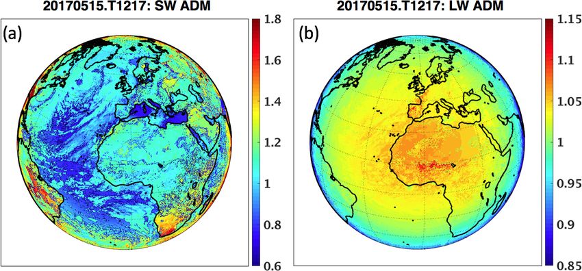
NISTAR measures an irradiance at the L1 point at a small
relative azimuth angle, φo , which varies from 4 to 15◦ , as
shown in Fig. 1a. As such, the radiation it measures comes
Figure 1. Schematic of the (a) Earth–Sun–DSCOVR geometry and from the near-backscatter position, which is different from
(b) Earth disk visible to the L1 DSCOVR view (left with an area
that seen at other satellite positions, as indicated in Fig. 1a
fraction of At ) and to the L2 view (right). The golden area on the left
shows the daytime area fraction (Av ) visible to DSCOVR, the black
by the varying arrow lengths corresponding to scattering an-
area on the left shows the night portion (Ad ) within the DSCOVR gles, 21 − 23 . Other types of Earth-orbiting satellites view
view, and the golden area on the right is the daytime portion (Ah ) a given spot on the Earth from various scattering angles that
missed by DSCOVR. Not to scale. vary as a function of local time (e.g., geostationary) or over-
pass time (e.g., Sun-synchronous). When averaged over the
globe, the uncertainties in the anisotropy corrections are mit-
aerosol–cloud interactions (e.g., Loeb and Schuster, 2008; igated by compensation. That is, any small biases at partic-
Quaas et al., 2008; Su et al., 2010b), as well as evaluating ular angles are balanced by observations taken at other an-
global general circulation models (e.g., Pincus et al., 2008; gles. In contrast, instruments on DSCOVR view every spot
Su et al., 2010a; Wang and Su, 2013; Wild et al., 2013). on the Earth from a single scattering angle that varies slowly
The Earth’s radiative flux data record is augmented by within a small range over the course of the Lissajous orbit.
the Deep Space Climate Observatory (DSCOVR) launched Thus, the correction for anisotropy is critical. The biases in
on 11 February 2015. DSCOVR is designed to continuously the anisotropy correction for the DSCOVR scattering angle
monitor the sunlit side of the Earth, being the first Earth- are mitigated and potentially minimized by the wide range
observing satellite at the Lagrange-1 (L1) point, ∼ 1.5 mil- of different scene types viewed in a given NISTAR measure-
lion km from Earth, where it orbits the Sun at the same rate as ment (Su et al., 2018).
the Earth (see Fig. 1a). DSCOVR is in an elliptical Lissajous Su et al. (2018) described the methodology to derive the
orbit around the L1 point and is not positioned exactly on global mean daytime shortwave (SW) anisotropic factors
the Earth–Sun line; therefore, only about 92 %–97 % of the by using the CERES angular distribution models (ADMs)
sunlit Earth is visible to DSCOVR. As illustrated in Fig. 1b, and a cloud property composite based on lower-Earth or-
the daytime portion (Ah ) is not visible to DSCOVR. Strictly bit satellite imager retrievals. These SW anisotropic factors
speaking, the measurements from DSCOVR are not truly were applied to EPIC broadband SW radiances, which were
“global” daytime measurements. However, for simplicity we estimated from EPIC narrowband observations based upon
refer to them as global daytime measurements. Onboard narrowband-to-broadband regressions, to derive the global
DSCOVR, the National Institute of Standards and Tech- daytime SW fluxes. Daily mean EPIC and CERES SW fluxes
nology Advanced Radiometer (NISTAR) provides continu- calculated using concurrent hours agree with each other to
ous full-disk global broadband irradiance measurements over within 2 %. They concluded that the SW flux agreement is
most of the sunlit side of the Earth (viewing the sunlit side of within the calibration and algorithm uncertainties, which in-
the Earth as one pixel). Besides NISTAR, DSCOVR also car- dicates that the method developed to calculate the global
ries the Earth Polychromatic Imaging Camera (EPIC), which anisotropic factors from the CERES ADMs is robust and
provides 2048 by 2048 pixel imagery 10 to 22 times per day that the CERES ADMs accurately account for the Earth’s
in 10 spectral bands from 317 to 780 nm. On 8 June 2015, anisotropy in the near-backscatter direction.
more than 100 d after launch, DSCOVR started orbiting In this paper, the same global daytime mean anisotropic
around the L1 point. factors developed by Su et al. (2018) are applied to the
The NISTAR instrument was designed to measure the NISTAR measurements to derive the global daytime mean
global daytime shortwave (SW) and longwave (LW) radia- SW and longwave (LW) fluxes. The NISTAR data and the
tive fluxes. The original objective of NISTAR was to moni- unfiltering algorithms developed for the NISTAR shortwave
Atmos. Meas. Tech., 13, 429–443, 2020 www.atmos-meas-tech.net/13/429/2020/
W. Su et al.: Determining the daytime Earth radiative flux                                                                     431

and near-infrared channels are detailed in Sect. 2. The data       ment noise level and the relatively short time allotted to the
and methodology used to derive the global daytime mean             space views.
anisotropic factors are presented in Sect. 3. Hourly daytime           NISTAR Level 1B radiometric products are derived by
SW and LW fluxes calculated from NISTAR measurements               first subtracting the offsets from Earth-view measurements
and comparisons with the CERES synoptic flux products              and then dividing by the laboratory-measured responsivity.
(SYN1deg; Doelling et al., 2013) are detailed in Sect. 4, fol-     The result is irradiance measured at the instrument aperture.
lowed by conclusions and a discussion in Sect. 5.                  Radiance (I ) is then calculated from the irradiance data and
                                                                   the solid angle (2) determined from the DSCOVR-to-Earth
                                                                   distance and the Earth dimensions. When averaging over a
2   NISTAR observation                                             4 h period, the NISTAR total and SW channel uncertainties
                                                                   (k = 1) are 1.5 % and 2.1 %, respectively. As the LW is de-
The NISTAR instrument measures Earth irradiance data for           rived from the difference between the total and unfiltered
an entire hemisphere using cavity electrical substitution ra-      SW channels, it contains noise contributions from both. The
diometers (ESRs) and filters covering three channels: short-       LW uncertainty is about 3.3 % (8 Wm−2 ) given that the day-
wave (SW, 0.2–4.0 µm), near-infrared (NIR, 0.7–4.0 µm),            time mean LW and SW fluxes are approximately 210 and
and total (0.2–100 µm). Each channel has a dedicated ESR           240 Wm−2 , respectively, and that the uncertainties between
that by itself is sensitive to radiation from 0.2 to 100 µm. For   the total and SW channels are largely uncorrelated.
the NIR and SW channels, filters are positioned in front of            As mentioned before, filters are placed in front of the ra-
each ESR to limit the incident radiation to spectral bands.        diometers to measure the energies from the SW and NIR por-
The filters reside in a filter wheel that, during normal oper-     tions of the spectrum. Since no corrections for the impact of
ation, configures each ESR to measure contemporaneously            filter transmission were applied to the NISTAR L1B data, the
in a different band. Additionally, each ESR has a shutter          SW and NIR radiances from NISTAR must first be unfiltered
that modulates the Earth signal by cycling between open and        before they can be used to derive the daytime Earth radia-
closed states continually with a 50 % duty cycle and a period      tive flux. Here we follow the algorithm developed by Loeb
of 4 min. The modulation is necessary as the ESRs only mea-        et al. (2001) to convert measured NISTAR-filtered radiances
sure changes in the incident optical power and, being thermal      to unfiltered radiances.
detectors, they have large offsets (background signals) that           Unfiltered SW and NIR radiances are defined as follows:
drift over relatively short time frames (hours) but not signifi-             Z λ2
cantly over a shutter cycle. Demodulating the resulting signal       band
                                                                   Iu =           Iλ dλ,                                       (1)
removes those offsets and the associated drifts and/or noise.                λ1
What remains is a much more stable shutter-modulated back-         where “band” represents either SW or NIR, λ(µm) is the
ground that is measured during periodic views of dark space        wavelength, and Iλ (Wm−2 sr−1 µm−1 ) is the spectral SW
and subsequently subtracted from the signal. The shutter-          radiance. The filtered radiance is the radiation that passes
modulated background is largest for the total channel and          through the spectral filter and is measured by the detector:
much smaller for the SW and NIR channels.
                                                                            Z λ2
   The NISTAR-calibrated Level 1B data products are de-
rived from prelaunch system-level optical calibration and on-      Ifband =      Sλband Iλ dλ,                                (2)
                                                                             λ1
orbit offset measurements. The former involved optical re-
sponse measurements of each active cavity radiometer with-         where Sλband is the spectral transmission function. Figure 2
out a filter in place using a narrowband calibration source        shows the NISTAR SW and NIR spectral transmission func-
whose irradiance was measured with a NIST-calibrated (Na-          tions. These functions are determined from ground testing
tional Institute of Standards and Technology) reference de-        done in 1999 and 2010 at the National Institute of Standards
tector. Those measurements establish the irradiance respon-        and Technology (NIST). The spectral radiance database is
sivity of each spectrally flat broadband radiometer. Addi-         calculated using a high-spectral-resolution radiative transfer
tionally, measurements of the transmittance of the SW and          model (Kato et al., 2002). Unfiltered radiances are deter-
NIR filters were made. This was done at NIST prior to in-          mined by integrating spectral radiances over the appropriate
stallation into the NISTAR filter wheel at wavelengths rang-       wavelength intervals using Gaussian quadrature. Similarly,
ing from 200 nm to approximately 18 µm. Further, system-           filtered radiances are computed by integrating over the prod-
level filter transmittance measurements at discrete visible and    uct of spectral radiance and spectral transmission function.
near-infrared wavelengths were made using the external light       The calculations are done for 480 angles: 6 solar zenith an-
source and the NISTAR photodiode channel as a detector.            gles (0.0, 29.0, 41.4, 60.0, 75.5, 85.0◦ ), 8 viewing zenith an-
The two transmittance measurements agreed to within a few          gles (0, 12, 24, 36, 48, 60, 72, 84◦ ), and 10 relative azimuth
tenths of a percent. Radiometric offsets are measured on-          angles (0 to 180, at every 20◦ ).
orbit monthly when NISTAR briefly views dark space. The                The database includes spectral radiances calculated over
offset measurement uncertainty is determined by the instru-        ocean, land–desert, and snow–ice surfaces for clear and

www.atmos-meas-tech.net/13/429/2020/                                                   Atmos. Meas. Tech., 13, 429–443, 2020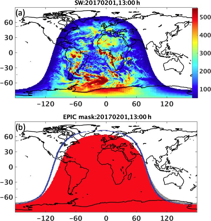
432                                                                  W. Su et al.: Determining the daytime Earth radiative flux

Table 1. Summary of the cases included in the spectral radiance database. AOD is for aerosol optical depth, and COD is for cloud optical
depth.

                                                                      Clear
                                        AOD     Aerosol type         Surface     Atmosphere
                              Ocean         8   Maritime tropical         4      Standard
                              Land          6   Continental              15      Standard
                              Snow          5   Continental               2      Arctic winter and summer
                                                                     Cloudy
                                        COD     Cloud type           Surface     Atmosphere
                              Ocean         7   4 liquid and 3 ice        4      Standard
                              Land          7   4 liquid and 3 ice       15      Standard

                                                                      tropical aerosol type for clear ocean, only changes the ratios
                                                                      to the fourth decimal point. As the ratio is not sensitive to the
                                                                      scene type and the Sun-viewing geometry, the SW unfiltering
                                                                      for NISTAR can be accomplished by
                                                                                Ifsw
                                                                      Iusw =            ,                                           (3)
                                                                                κ sw
                                                                      where Ifsw represents the filtered radiances directly from the
                                                                      NISTAR L1B data. As the NISTAR view always contains
                                                                      clouds, we choose to use the mean ratios of the cloudy ocean
                                                                      and land cases in Table 2, which is 0.8690 for the SW band.
Figure 2. NISTAR SW and NIR spectral transmission function.           The estimated uncertainty of using this single ratio for unfil-
                                                                      tering the SW band is less than 0.3 %.
                                                                         On the other hand, the variability in the ratios of the NIR
                                                                      band can be as large as 6 %. Fortunately, the large variabil-
cloudy conditions. Table 1 summarizes the numbers of each             ity only occurs between clear ocean and clear land. As men-
variable that are included in the database; there are a total of      tioned earlier, the NISTAR view always contains clouds, and
142 clear-sky cases and a total of 931 cloudy-sky cases for           the mean ratios of the cloudy ocean and land cases, which
each Sun-viewing geometry. This is a much larger database             is 0.8583, is used to unfilter the NISTAR NIR observations.
compared with that used by Loeb et al. (2001).                        This mean ratio can differ with the individual ratios for dif-
    For CERES unfiltering, regression coefficients between            ferent solar zenith angles under cloudy conditions by about
filtered and unfiltered radiances were derived as functions of        1 %–2 %. The mean ratio of the NIR bands is used to convert
scene type and Sun-viewing geometry (Loeb et al., 2001).              the filtered radiances to unfiltered radiances:
Given that NISTAR views the Earth as a single pixel, a mix
of scenes and many Sun-viewing geometries are observed at                       Ifnir
                                                                      Iunir =           .                                           (4)
the same time. The method used for CERES is not feasible                        κ nir
for unfiltering NISTAR observations. We instead investigated
                                                                      In this paper, the measurements from the NISTAR NIR chan-
the feasibility of using the ratio, κ, between filtered and un-
                                                                      nel are not used. The unfiltering of the NIR channel is re-
filtered radiances for unfiltering the NISTAR observations.
                                                                      ported here for readers who intend to use this channel.
Table 2 lists the mean and the standard deviations of the ra-
                                                                         As there is no filter placed in front of the total channel, the
tios at different solar zenith angles. The ratios for the SW
                                                                      radiance from the total channel does not need to be unfiltered.
band are extremely stable, varying less than 0.3 % among the
                                                                      The LW (4–100 µm) radiance can be derived by subtracting
scenes and Sun-viewing geometries considered (the small-
                                                                      the unfiltered SW radiance from the total:
est ratio, 0.8659, occurs for clear ocean under overhead Sun
and the largest ratio, 0.8694, occurs for clear or cloudy land        Iulw = I tot − Iusw .                                         (5)
under overhead Sun). Furthermore, the ratios are not sensi-
tive to the atmospheric profile and the aerosol type used. For        The unfiltered radiances (Iusw and Iulw ) will be used hereafter
example, using a tropical profile instead of the standard at-         to derive the daytime mean radiative flux. Although NISTAR
mosphere, and using the maritime clean instead of maritime            L1B data provide observations every second, hourly data

Atmos. Meas. Tech., 13, 429–443, 2020                                                         www.atmos-meas-tech.net/13/429/2020/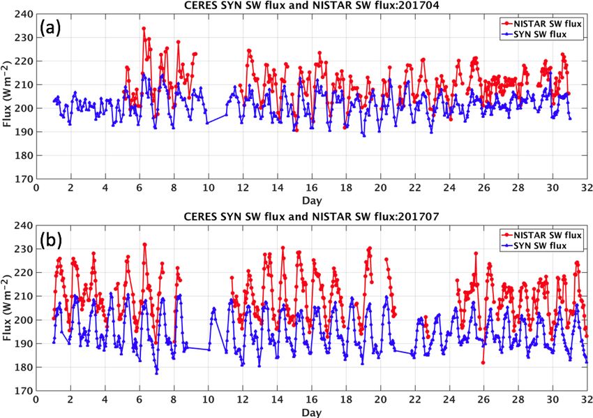
W. Su et al.: Determining the daytime Earth radiative flux                                                                                     433

Table 2. Mean ratio and standard deviation (in parenthesis) of filtered radiance to unfiltered radiance for SW and NIR bands over different
scene types.

             SW ratio (standard deviation ×1000)
                                      0.0             29.0             41.4            60.0                      75.5             85.0
             Clear ocean     0.8659 (1.0)     0.8660 (1.0)     0.8661 (1.1)    0.8664 (1.2)         0.8669 (1.0)         0.8674 (0.8)
             Clear land      0.8694 (0.6)     0.8693 (0.6)     0.8692 (0.6)    0.8690 (0.5)         0.8687 (0.5)         0.8685 (0.8)
             Clear snow      0.8689 (0.1)     0.8689 (0.1)     0.8689 (0.2)    0.8688 (0.2)         0.8688 (0.3)         0.8687 (0.4)
             Cld ocean       0.8687 (1.0)     0.8687 (1.0)     0.8688 (0.9)    0.8688 (0.8)         0.8688 (0.7)         0.8687 (0.6)
             Cld land        0.8694 (0.4)     0.8693( 0.3)     0.8693 (0.3)    0.8692 (0.3)         0.8690 (0.4)         0.8689 (0.5)
             NIR ratio (standard deviation ×1000)
                                      0.0             29.0             41.4            60.0                      75.5             85.0
             Clear ocean    0.8293 (23.1)    0.8270 (24.0)   0.8253 (25.5)    0.8235 (28.3)        0.8238 (28.4)        0.8229 (26.4)
             Clear land      0.8790 (9.6)    0.8777 (10.4)   0.8764 (10.7)    0.8730 (10.8)        0.8663 (10.1)        0.8501 (12.4)
             Clear snow      0.8360 (1.7)     0.8360 (1.8)    0.8361 (1.9)     0.8363 (2.1)         0.8370 (2.8)         0.8365 (6.0)
             Cld ocean       0.8557 (3.2)     0.8555 (2.6)    0.8562 (2.4)     0.8567 (3.1)         0.8565 (4.4)         0.8539 (7.9)
             Cld land        0.8627 (8.2)     0.8624 (7.8)    0.8621 (7.3)     0.8613 (6.2)         0.8598 (4.8)         0.8566 (6.2)

(smoothed with 4 h running mean) are used to derive fluxes              lated, and all radiances in the upwelling directions are inte-
because of the level of noise presented in the measurements             grated to provide the ADM flux (F̂ ). The ADM anisotropic
(DSCOVR NISTAR data quality report v02).                                factors (R) for scene type χ are then calculated as

                                                                                                            π Iˆ(θ0 , θ, φ, χ )
3     Global daytime shortwave and longwave anisotropic                 R(θ0 , θ, φ, χ ) = R R       π
                                                                                            2π
                                                                                              0     0
                                                                                                     2
                                                                                                         Iˆ(θ0 , θ, φ, χ ) cos θ sin θ dθ dφ
      factors
                                                                                            π Iˆ(θ0 , θ, φ, χ )
To derive the global daytime mean SW and LW fluxes from                                 =                           ,                          (6)
                                                                                                  F̂ (θ0 , χ )
the NISTAR unfiltered radiances, the anisotropy of the TOA
radiance field must be considered. The CERES Edition 4 em-              where θ0 is the solar zenith angle, θ is the CERES view-
pirical ADMs and a cloud property composite based upon                  ing zenith angle, and φ is the relative azimuth angle between
lower-Earth orbit satellite retrievals are used here to estimate        CERES and the solar plane.
the global mean shortwave and longwave anisotropic factors.
                                                                        3.2   EPIC composite data
3.1    CERES ADMs
                                                                        As stated in the section above, the anisotropy of the radi-
The Edition 4 CERES ADMs (Su et al., 2015) are con-                     ation field at the TOA was constructed for different scene
structed using the CERES observations taken during the ro-              types, which were defined using many variables including
tating azimuth plane (RAP) scan mode. In this mode, the in-             cloud properties such as cloud fraction, cloud optical depth,
strument scans in elevation as it rotates in azimuth, thus ac-          and cloud phase (Loeb et al., 2005; Su et al., 2015). Al-
quiring radiance measurements from a wide range of view-                though the EPIC L2 cloud product includes a threshold-based
ing combinations. The CERES ADMs are derived for various                cloud mask, which identifies the EPIC pixels as high confi-
scene types, which are defined using a combination of vari-             dent clear, low confident clear, high confident cloudy, and
ables (e.g., surface type, cloud fraction, cloud optical depth,         low confident cloudy (Yang et al., 2019), the low resolution
cloud phase, aerosol optical depth, precipitable water, lapse           of EPIC imagery (24 × 24 km2 ) and its lack of infrared chan-
rate, etc). To provide accurate scene-type information within           nels diminish its capability to identify clouds and to accu-
CERES footprints, imager (Moderate Resolution Imaging                   rately retrieve cloud properties. As EPIC lacks the channels
Spectroradiometer – MODIS – on Terra and Aqua), cloud,                  that are suitable for cloud size and phase retrievals (Meyer
and aerosol retrievals (Minnis et al., 2010, 2011) are aver-            et al., 2016), two cloud optical depths are determined assum-
aged over CERES footprints by accounting for the CERES                  ing the cloud phase is liquid or ice using a constant cloud ef-
point spread function (PSF, Smith, 1994) and are used for               fective radius (14 µm for liquid and 30 µm for ice) for cloudy
scene-type classification. Over a given scene type (χ), the             EPIC pixels. These cloud properties are not sufficient to pro-
CERES-measured radiances are sorted into discrete angular               vide the scene-type information necessary for ADM selec-
bins. Averaged radiances (Iˆ) in all angular bins are calcu-            tions. Therefore, more accurate cloud property retrievals are

www.atmos-meas-tech.net/13/429/2020/                                                              Atmos. Meas. Tech., 13, 429–443, 2020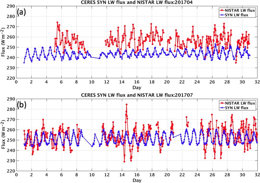
434                                                                W. Su et al.: Determining the daytime Earth radiative flux

needed to provide anisotropy characterizations to convert ra-       the global and EPIC composites are provided in Khlopenkov
diances to fluxes.                                                  et al. (2017).
   To accomplish this, we take advantage of the cloud prop-            Figure 3a shows an image from EPIC taken on
erty retrievals from multiple imagers on low-Earth orbit            15 May 2017 at 12:17 UTC; the corresponding total cloud
(LEO) satellites and geostationary (GEO) satellites. The            fraction (the sum of liquid and ice cloud fractions) from
LEO satellite imagers include MODIS on the Terra and Aqua           the EPIC composite is shown in Fig. 3b. The liquid and ice
satellites, the Visible Infrared Imaging Suite (VIIRS) on           cloud fraction, optical depth, and effective height are shown
the Suomi-National Polar-orbiting Partnership satellite, and        in Fig. 3c–h. For this case, most of the clouds are in the liquid
the Advanced Very High Resolution Radiometer (AVHRR)                phase. Optically thick liquid clouds with effective heights of
on the NOAA and MetOps platforms. The GEO imagers                   2 to 4 km are observed in the northern Atlantic Ocean and in
are on the Geostationary Operational Environmental Satel-           the Arctic. Ice clouds with effective heights of 8 to 10 km are
lites (GOES), the Meteosat series, and Himawari-8 to pro-           observed off the west coast of Africa and Europe.
vide semi-global coverage. All cloud properties were deter-
mined using a common set of algorithms, the Satellite ClOud         3.3    Calculating global daytime anisotropic factors
and Radiation Property retrieval System (SatCORPS; Min-
nis et al., 2008a, 2016), based on the CERES cloud detec-           To determine the global daytime mean anisotropic factors,
tion and retrieval system (Minnis et al., 2008b, 2010, 2011).       we use the anisotropies characterized in the CERES ADMs,
Cloud properties from these LEO–GEO imagers are opti-               and they are selected based upon the scene-type information
mally merged together to provide a seamless global compos-          provided by the EPIC composite for every EPIC FOV. For
ite product at 5 km resolution by using an aggregated rating        a given EPIC FOV (j ), its anisotropic factor is determined
that considers five parameters (nominal satellite resolution,       based upon the Sun–EPIC viewing geometry and the scene
pixel time relative to the EPIC observation time, viewing           identification information provided by the EPIC composite:
zenith angle, distance from day–night terminator, and Sun                                          π Iˆj (θ0 , θ e , φ e , χ e )
glint factor to minimize the usage of data taken in the glint       Rj (θ0 , θ e , φ e , χ e ) =                                 ,    (7)
region) and selects the best observation at the time nearest the                                         Fˆj (θ0 , χ e )
EPIC measurements. About 80 % of the LEO–GEO satellite              where θ e is the EPIC viewing zenith angle, φ e is the rela-
overpass times are within 40 min of the EPIC measurements,          tive azimuth angle between EPIC and the solar plane, and
while 96 % are within 2 h of the EPIC measurements. Most            χ e is the scene identification from the EPIC composite. Here
of the regions covered by GEO satellites (between around            Iˆj is the radiance from CERES ADMs and F̂j is the flux
50◦ S and 50◦ N) have a very small time difference, in the          from CERES ADMs (see Eq. 6). To derive the global mean
range of ±30 min, because of the availability of hourly GEO         anisotropic factor, we follow the method developed by Su
observations. The polar regions are also covered very well by       et al. (2018) and calculate the global daytime mean ADM
polar orbiters. Thus, larger time differences generally occur       radiance as
over the 50 to 70◦ latitude regions. Given the temporal reso-             PN
                                                                                   ˆ        e e     e
lution of the currently available GEO–LEO satellites, this is        ˆ       j =1 Ij (θ0 , θ , φ , χ )
                                                                    I=                                 .                      (8)
the best collocation possible for those latitudes.                                     N
   The global composite data are then remapped into the             To calculate the global mean ADM flux, we first grid the
EPIC field of view (FOV) by convolving the high-resolution          ADM flux (F̂ ) for each EPIC pixel into 1◦ latitude by 1◦
cloud properties with the EPIC point spread function (PSF)          longitude bins (F̂ (lat, lon)). These gridded ADM fluxes are
defined with a half-pixel accuracy to produce the EPIC com-         then weighted by the cosine of latitude to provide the global
posite. As the PSF is sampled with half-pixel accuracy, the         daytime mean ADM flux:
nominal spacing of the PSF grid is about the same size                   PM
as in the global composite data. Thus, the accuracy of the                  j =1 F̂j (lat, lon) cos(latj )
cloud fraction in the EPIC composite is not degraded com-           F̂ =           P                       .                  (9)
                                                                                       cos(latj )
pared to the global composite (Khlopenkov et al., 2017).
PSF-weighted averages of radiances and cloud properties are         The global mean anisotropic factor is calculated as
computed separately for each cloud phase because the LEO–
GEO cloud products are retrieved separately for liquid and                 π Iˆ
                                                                    R=            .                                                  (10)
ice clouds (Minnis et al., 2008a). Ancillary data (i.e., sur-              F̂
face type, snow and ice map, skin temperature, precipitable
water, etc.) needed for anisotropic factor selections are also      We use Rsw and Rlw to denote the mean SW and LW
included in the EPIC composite. These composite images              anisotropic factors. The mean SW anisotropic factor is then
are produced for each observation time of the EPIC instru-          used to convert the NISTAR SW unfiltered radiance to flux:
ment (typically 300 to 600 composites per month). Detailed                      π Iusw
descriptions of the method and the input used to generate           Fnsw =               .                                           (11)
                                                                                Rsw

Atmos. Meas. Tech., 13, 429–443, 2020                                                        www.atmos-meas-tech.net/13/429/2020/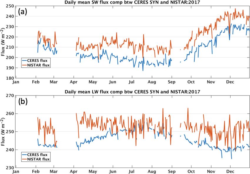
W. Su et al.: Determining the daytime Earth radiative flux 435
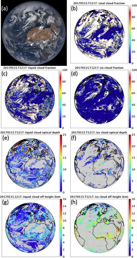
Figure 4. SW anisotropic factors (a) and LW anisotropic factors
(b) derived from the CERES ADMs using the EPIC composite for
scene identification for 15 May 2017 at 12:17 UTC.
larger over clear regions than over cloudy regions because of
the hot spot effect, which leads to anisotropic factors greater
than 1.6 over clear land regions at large viewing zenith an-
gles. The LW anisotropic factors show much less variabil-
ity compared to the SW anisotropic factors, with limb dark-
ening being the dominant feature. The mean SW and LW
anisotropic factors for this case are 1.275 and 1.041, respec-
tively.
4 NISTAR shortwave and longwave flux
The temporal resolution of the NISTAR Level 1B data
is 1 s; however, meaningful changes in the data only oc-
cur over many shutter cycles (each shutter cycle is 4 min)
due to the demodulation algorithm, which includes a box-
car filter having the width of a shutter period. The filter
reduces noise and rejects higher harmonics of the shut-
ter frequency. Following demodulation, significant instru-
ment noise remains. Therefore, further averaging in time
over a minimum of 2 h is recommended to further reduce
the noise levels (https://eosweb.larc.nasa.gov/project/dscovr/
DSCOVR_NISTAR_Data_Quality_Report_V02.pdf, last ac-
Figure 3. EPIC RGB image for 15 May 2017 at 12:17 UTC (a) cess: 24 January 2020). In this study, we use hourly radi-
and the corresponding total cloud fraction (b; %). Liquid and ice ances averaged from 4 h running means as suggested by the
cloud fractions are shown in (c) and (d), liquid and ice cloud optical NISTAR instrument team. The hours that are coincident with
depths are shown in (e) and (f), and liquid and ice cloud effective
the EPIC image times are converted to fluxes using the global
height (km) are shown in (g) and (h). Panels (b) to (h) are all derived
anisotropic factors calculated using the EPIC composites for
from the EPIC composite. Figure 3a is taken from: https://epic.gsfc.
nasa.gov (last access: 29 January 2020). scene identification. Figure 5 shows the hourly SW and LW
fluxes derived from NISTAR for April (a) and July (b) 2017.
For both months, the SW fluxes fluctuate around 210 Wm−2 ,
The LW flux is similarly derived from the following: with the difference between the daily maximum and mini-
mum as large as 30 Wm−2 . The LW fluxes fluctuate around
π Iulw 260 Wm−2 and exhibit surprisingly large diurnal variations.
Fnlw = . (12) These NISTAR fluxes are compared to the CERES synop-
Rlw
tic radiative fluxes and clouds product (SYN1deg; Doelling
Figure 4 shows an example of SW and LW anisotropic et al., 2013), which provides hourly cloud properties and
factors for every EPIC FOV. The SW anisotropic factors are fluxes for each 1◦ latitude by 1◦ longitude. Within the
generally smaller over clear than over cloudy oceanic re- SYN1deg data product, fluxes between CERES observations
gions. Over land, however, the SW anisotropic factors are are inferred from hourly GEO visible and infrared imager
www.atmos-meas-tech.net/13/429/2020/ Atmos. Meas. Tech., 13, 429–443, 2020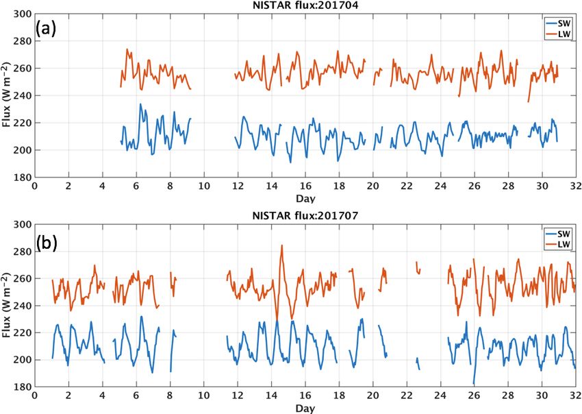
436                                                                W. Su et al.: Determining the daytime Earth radiative flux

Figure 5. SW flux (blue) and LW flux (red) derived from NISTAR measurements for April (a) and July (b) 2017.

measurements between 60◦ S and 60◦ N using observation-              mean daytime fluxes that are comparable to those from the
based narrowband-to-broadband radiance and radiance-to-              NISTAR measurements:
flux conversion algorithms. However, the GEO narrowband                    P
                                                                              Fj cos(latj )ωj
channels have a greater calibration uncertainty than MODIS           Fsyn = P                 .                           (13)
                                                                               cos(latj )ωj
and CERES. Several procedures are implemented to ensure
consistency between the MODIS-derived and GEO-derived                Here, Fj is the gridded hourly CERES SYN fluxes, “lat”
cloud properties and between the CERES fluxes and the                is the latitude, and ω indicates whether a grid box is visi-
GEO-based fluxes. These include calibrating GEO visible              ble to NISTAR (1 when visible, 0 when not visible). Fig-
radiances against the well-calibrated MODIS 0.65 µm radi-            ure 6a shows an example of the gridded SYN SW fluxes at
ances by ray-matching MODIS and GEO radiances; apply-                13:00 UTC on 1 February 2017. SW fluxes for the daytime
ing similar cloud retrieval algorithms to derive cloud prop-         grid boxes are shown in color, while all nighttime grid boxes
erties from MODIS and GEO observations; and normaliz-                are shown in white. Figure 6b shows the daytime areas (in
ing GEO-based broadband fluxes to CERES fluxes using co-             red) and the nighttime areas (in grey) visible to the NISTAR
incident measurements. Comparisons with broadband fluxes             view. Daytime areas of northern high latitudes and North
from the Geostationary Earth Radiation Budget (GERB; Har-            America are not within the NISTAR view and are therefore
ries et al., 2005) indicate that SYN1deg hourly fluxes are           not included in the comparison with the NISTAR fluxes, and
able to capture the subtle diurnal flux variations. Compar-          the nighttime slivers in the southern high latitudes of the In-
ing with the GERB fluxes, the bias of the SYN SW fluxes is           dian Ocean and Pacific Ocean are included in the LW flux
1.3 Wm−2 , the monthly regional all-sky SW flux root mean            comparison with NISTAR.
square (RMS) error is 3.5 W m−2 , and the daily regional all-           Figure 7 compares the SW fluxes from NISTAR with
sky SW flux RMS error is 7.8 W m−2 (Doelling et al., 2013).          those from the CERES SYN1deg product integrated for the
These uncertainties could be overestimated, as the GERB do-          NISTAR view (Eq. 19) for April (a) and July (b) 2017. The
main has a disproportionate number of strong diurnal cycle           CERES SW fluxes oscillate around 200 and 195 Wm−2 for
regions compared with the globe.                                     April and July, whereas the NISTAR counterparts are about
   To account for the missing energy from the daytime por-           10 to 20 Wm−2 greater. The maxima and minima of SW
tion that is not observed by NISTAR (Ah in Fig. 1b) and              fluxes from NISTAR align well with those from CERES,
the energy from the nighttime sliver within the DSCOVR               though the differences between the daily maximum and min-
view (Ad in Fig. 1b; only applicable to LW flux), the hourly         imum from NISTAR appear to be larger than those from
gridded SYN fluxes are integrated by considering only the            CERES. The diurnal variations of SW flux derived from
grid boxes that are visible to NISTAR to produce the global          EPIC showed a much better agreement with those from
                                                                     CERES (Su et al., 2018). The exact cause for these larger di-

Atmos. Meas. Tech., 13, 429–443, 2020                                                    www.atmos-meas-tech.net/13/429/2020/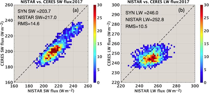
W. Su et al.: Determining the daytime Earth radiative flux                                                                       437

                                                                     SW fluxes from NISTAR are highly correlated (correlation
                                                                     coefficient of about 0.89) with those from CERES SYN1deg,
                                                                     but the correlation for the LW fluxes is rather low (correlation
                                                                     coefficient is about 0.38). Note that when inverting fluxes
                                                                     from hourly mean NISTAR radiances (instead of 4 h running
                                                                     mean radiances), it changed the monthly mean SW and LW
                                                                     fluxes by less than 1.0 and 0.5 Wm−2 , respectively. However,
                                                                     the RMS errors increased for both SW and LW fluxes due to
                                                                     the noise presented in the NISTAR observation.
                                                                        NISTAR fluxes derived at the EPIC image times are aver-
                                                                     aged into daily means and compared with the daily means
                                                                     from CERES SYN1deg using concurrent hours (Fig. 10).
                                                                     The NISTAR SW fluxes are consistently higher than those
                                                                     from CERES by about 10 to 15 Wm−2 . CERES SW fluxes
                                                                     show a strong annual cycle, which is driven by the incident
                                                                     solar radiation that is affected by the Earth–Sun distance.
                                                                     This annual cycle is also evident in the NISTAR SW fluxes,
                                                                     although the fluxes during the period from April to August
                                                                     are flatter than those from CERES. The NISTAR LW fluxes
                                                                     are greater than those from CERES except during the boreal
                                                                     summer months, with the largest difference of 10 Wm−2 in
                                                                     February and the smallest difference of a few Watts per me-
Figure 6. An example of the daytime SW flux distributions from the   ter during the boreal summer months. The CERES LW fluxes
CERES SYN1deg product at 13:00 UTC on 1 February 2017 (a)
                                                                     show an annual cycle of about 10 Wm−2 , with the largest
and the corresponding daytime areas (in red) and nighttime areas
(in grey) that are visible to NISTAR and the terminator boundary
                                                                     LW fluxes occurring during the boreal summer when the
(in blue) (b).                                                       vast landmasses of the Northern Hemisphere are warmer than
                                                                     during the other seasons. The annual cycle of the NISTAR
                                                                     LW fluxes shows less seasonal variation. From April to Octo-
                                                                     ber, the NISTAR LW fluxes oscillate around 255 Wm−2 , and
urnal variations from the NISTAR SW flux is not known. LW            they oscillate around 250 Wm−2 for other months. Addition-
flux comparisons are shown in Fig. 8. The daily maximum–             ally, the CERES LW fluxes exhibit much smaller day-to-day
minimum LW differences from CERES are typically less                 variations than their NISTAR counterparts. Note that some
than 15 Wm−2 and exhibit small day-to-day and month-to-              of the variations of daily mean fluxes shown in Fig. 10 are
month variation. However, the daily maximum–minimum                  due to temporal sampling changes when data transmissions
LW differences from NISTAR can vary from 10 to 50 Wm−2 .             encountered difficulties and/or during spacecraft maneuvers.
This larger than expected variability of NISTAR LW fluxes
is due to the fact that noise and offset variabilities from
both the NISTAR total and SW channel are present in the              5   Conclusions and discussion
NISTAR LW radiances. The NISTAR LW fluxes are con-
sistently greater than CERES LW fluxes by about 10 to                The SW radiances included in the NISTAR L1B data are
20 Wm−2 in April. The LW fluxes agree better for July, but           filtered radiances, and the effect of the filter transmission
the NISTAR LW fluxes show larger diurnal variations than             must be addressed before these measurements can be used
the CERES fluxes.                                                    to derive any meaningful fluxes. A comprehensive spectral
   Figure 9 compares the SW and LW fluxes from the CERES             radiance database has been developed to investigate the rela-
SYN1deg product with those from NISTAR at all coinci-                tionship between filtered and unfiltered radiances using the-
dent hours of 2017. The mean SW fluxes are 203.7 and                 oretically derived values simulated for typical Earth scenes
217.0 Wm−2 , respectively, for CERES and NISTAR, and the             and the NISTAR spectral transmission functions. The ratio
RMS error is 14.6 Wm−2 (Fig. 9a). The mean LW fluxes are             between filtered and unfiltered SW radiances is very sta-
246.0 and 252.8 Wm−2 for CERES and NISTAR, and the                   ble, varying less than 0.3 % for the scenes and the Sun-
RMS error is 10.5 Wm−2 (Fig. 9b). Tables 3 and 4 summa-              viewing geometries included in the database. The mean ratio
rize the flux comparisons between NISTAR and CERES for               of 0.8690 is used to derive the unfiltered SW radiance from
all months of 2017. The NISTAR SW fluxes are consistently            the NISTAR L1B filtered SW radiance measurements.
greater than those from CERES SYN1deg by about 3.4 % to                  To convert these unfiltered radiances into fluxes, the
7.8 %, and the NISTAR LW fluxes are also greater than those          anisotropy of the radiance field must be taken into ac-
from CERES SYN1deg by 1.0 % to 5.0 %. Furthermore, the               count. We use the scene-type-dependent CERES angular

www.atmos-meas-tech.net/13/429/2020/                                                     Atmos. Meas. Tech., 13, 429–443, 2020
438 W. Su et al.: Determining the daytime Earth radiative flux
Table 3. SW flux comparisons between NISTAR and CERES SYN1deg for all coincident observations of 2017. Fn is the NISTAR flux
(Wm−2 ), Fs is the SYN flux (Wm−2 ), and RMS is the root mean square error between them (Wm−2 ).
Jan Feb Mar Apr May Jun Jul Aug Sep Oct Nov Dec
Fs – 208.1 203.4 199.8 201.0 200.2 194.4 193.0 198.7 208..9 221.6 228.2
Fn – 218.5 215.4 211.5 214.1 213.5 209.2 208.7 211.2 222.8 235.1 240.0
RMS – 11.9 14.0 12.9 14.0 14.6 16.0 16.8 13.9 15.5 14.5 14.0
Table 4. LW flux comparisons between NISTAR and CERES SYN1deg for all coincident observations of 2017. Fn is the NISTAR flux
(Wm−2 ), Fs is the SYN flux (Wm−2 ), and RMS is the root mean square error between them (Wm−2 ).
Jan Feb Mar Apr May Jun Jul Aug Sep Oct Nov Dec
Fs – 242.0 241.1 243.0 246.3 249.1 251.5 248.9 245.5 242.9 239.8 240.6
Fn – 253.1 248.1 257.7 255.8 255.2 255.6 253.2 255.5 253.5 250.4 253.3
RMS – 13.4 10.0 16.0 11.5 10.3 8.7 10.0 12.2 12.5 12.4 14.4
distribution models to characterize the global SW and LW Furthermore, the NISTAR LW fluxes have very low corre-
anisotropy. These global anisotropies are calculated based lations with the CERES LW fluxes. NISTAR LW fluxes ex-
upon the anisotropies for each EPIC pixel. To accurately ac- hibit a nearly flat annual variation, whereas the CERES LW
count for the anisotropy for each EPIC pixel, an EPIC com- fluxes exhibit a distinct annual cycle, with the highest LW
posite was developed that includes all information needed flux occurring in July when the vast Northern Hemisphere
for angular distribution model selections. The EPIC compos- landmasses are warmest. The NISTAR LW fluxes also ex-
ite includes cloud property retrievals from multiple imagers hibit unrealistically large day-to-day variations.
on the LEO and GEO satellites. Cloud properties from these The SW flux discrepancy between NISTAR and CERES
LEO and GEO imagers are optimally merged together to pro- is caused by (1) CERES instrument calibration uncertainty,
vide a global composite product at 5 km resolution by using (2) CERES flux algorithm uncertainty, (3) NISTAR instru-
an aggregated rating that considers several factors and se- ment measurement uncertainty, and (4) NISTAR flux al-
lects the best observation at the time nearest the EPIC mea- gorithm uncertainty. The CERES SW channel calibration
surements. The global composite data are then remapped into uncertainty is 1 % (1σ ; McCarthy et al., 2011; Priestley
the EPIC FOV by convolving the high-resolution cloud prop- et al., 2011; Loeb et al., 2018), which corresponds to about
erties with the EPIC PSF to produce the EPIC composite. 2.1 Wm−2 for daytime mean SW fluxes. The CERES algo-
PSF-weighted averages of radiances and cloud properties are rithm uncertainty includes radiance-to-flux conversion error,
computed separately for each cloud phase, and ancillary data which is 1.0 Wm−2 according to Su et al. (2015), and diurnal
needed for anisotropic factor selections are also included in correction uncertainty, which is estimated to be 1.9 Wm−2
the EPIC composite. when Terra and Aqua are combined (Loeb et al., 2018).
These global anisotropies are applied to the NISTAR ra- The NISTAR SW channel measurement uncertainty is 2.1 %,
diances to produce the global daytime SW and LW fluxes, which corresponds to 4.4 Wm−2 . The NISTAR algorithm
and they are validated against the CERES synoptic 1◦ lati- uncertainty is essentially the radiance-to-flux conversion er-
tude by 1◦ longitude flux product. Only the grid boxes that ror. The estimation of this error source is not readily avail-
are visible to the NISTAR view are integrated to produce able given the unique NISTAR viewing perspective. How-
global mean daytime fluxes that are comparable to the fluxes ever, if we assume that the discrepancy between the EPIC-
from the NISTAR measurements. The NISTAR SW fluxes derived SW flux and CERES SW flux (Su et al., 2018) is
are consistently greater than those from CERES SYN1deg also from uncertainty sources (1) and (2) listed above, plus
by 10 to 15 Wm−2 (3.3 % to 7.8 %), but these two SW flux the EPIC calibration, narrowband-to-broadband conversion,
datasets are highly correlated, indicating that the diurnal and and radiance-to-flux conversion for EPIC, then we can de-
seasonal variations of the SW fluxes are fairly similar for duce that the radiance-to-flux conversion uncertainty for the
both of them. The NISTAR LW fluxes are also greater than NISTAR viewing geometry should be less than 2 Wm−2 .
those from CERES SYN1deg, but the magnitude of the dif- Thus, the total difference expected from these uncertainty
ference has larger month-to-month variations than that for sources should be (2.12 + 1.92 + 1.02 + 4.42 + 2.02 )1/2 =
the SW fluxes. The largest difference of about 14 Wm−2 5.7 Wm−2 .
(∼ 5.5 %) occurred in April 2017, and the smallest differ- Similarly, the LW flux discrepancy between NISTAR and
ence of about ∼ 4 Wm−2 (∼ 1.6 %) occurred during July. CERES is due to the same sources of error. The daytime
Atmos. Meas. Tech., 13, 429–443, 2020 www.atmos-meas-tech.net/13/429/2020/W. Su et al.: Determining the daytime Earth radiative flux 439 Figure 7. SW flux (Wm−2 ) comparisons between NISTAR and CERES SYN for April (a) and July (b) 2017. Figure 8. LW flux (Wm−2 ) comparisons between NISTAR and CERES SYN for April (a) and July (b) 2017. CERES LW flux uncertainty from calibration is 2.5 Wm−2 accuracy because of its Sun-synchronous orbit. Given that (1σ ; Loeb et al., 2009). The CERES LW radiance-to-flux NISTAR only views the Earth from the backscattering an- conversion error is about 0.75 Wm−2 (Su et al., 2015), and gles, the LW flux uncertainty due to radiance-to-flux con- diurnal correction uncertainty is estimated to be 2.2 Wm−2 version could be larger for the clear-sky footprints (Min- (Loeb et al., 2018). However, the CERES LW ADMs were nis et al., 2004). As the clear-sky occurrences are small at developed without taking the relative azimuth angle into con- the EPIC footprint size level, our best estimate of this un- sideration, which has little impact on the CERES LW flux certainty is no more than 0.4 Wm−2 . The calibration uncer- www.atmos-meas-tech.net/13/429/2020/ Atmos. Meas. Tech., 13, 429–443, 2020
440                                                             W. Su et al.: Determining the daytime Earth radiative flux

Figure 9. Comparison of coincident hourly SW and LW fluxes from NISTAR and CERES SYN1deg for 2017. The color bar indicates the
number of occurrences.

Figure 10. Daily mean SW flux (a) and LW flux (b) comparisons between CERES SYN1deg (blue) and NISTAR (red) for 2017.

tainty for NISTAR LW is deduced from the calibration un-          between CERES and NISTAR. The error sources related
certainties of total and SW channels. The total channel cal-      to NISTAR are preliminary and are under careful evalua-
ibration uncertainty is 1.5 %, which is about 6.8 Wm−2 as-        tion. Although the LW flux differences between CERES and
suming the total radiative energy of 450 Wm−2 . The SW            NISTAR are within the uncertainty estimation, the correla-
channel measurement uncertainty is 4.4 Wm−2 . The result-         tion between NISTAR and CERES is rather low, about 0.38.
ing LW channel measurement uncertainty is thus equal to           This is because the NISTAR LW radiance is derived as the
(6.82 + 4.42 )1/2 = 8.1 Wm−2 . Although no direct estimation      difference between total channel radiance and SW channel
of the radiance-to-flux conversion uncertainty for LW is          radiance; thus, the noise and offset variability of both the
available, we do not expect that it exceeds its SW counter-       NISTAR total and SW channels is present in the NISTAR
part of 2.0 Wm−2 . Thus, the total difference expected from       LW fluxes. As a result, more variability is expected in the
these uncertainty sources should be (2.52 + 0.752 + 0.42 +        LW data, which leads to the low correlation. Although the
2.22 + 8.12 + 2.02 )1/2 = 9.1 Wm−2 .                              noise level present in the NISTAR measurements prevents
   The uncertainty sources listed above can explain part of       the production of a high-frequency SW flux, the current 4 h
the SW flux differences and all of the LW flux differences        running mean fluxes are highly correlated with the CERES

Atmos. Meas. Tech., 13, 429–443, 2020                                               www.atmos-meas-tech.net/13/429/2020/
W. Su et al.: Determining the daytime Earth radiative flux                                                                                 441

product. The NISTAR SW flux can be used to test the diurnal               G., Smith, G. L., Szewczyk, Z. P., Mlynczak, P. E., Slingo, A.,
variations of SW flux in the high-temporal-resolution model               Allan, R. P., and Ringer, M. A.: The Geostationary Earth radia-
outputs from the Coupled Model Intercomparison Project.                   tion budget project, B. Am. Meteorol. Soc., 86, 945–960, 2005.
Furthermore, the spectral ratio information from NISTAR                 House, F. B., Gruber, A., Hunt, G. E., and Mecherikunnel, A. T.:
presents a new way to evaluate the models and opens a new                 History of satellite missions and measurements of the Earth radi-
                                                                          ation budget (1957–1984), Rev. Geophys., 24, 357–377, 1986.
perspective on exoplanet observations (Carlson et al., 2019).
                                                                        Kato, S., Loeb, N. G., and Rutledge, K.: Estimate of top-
                                                                          of-atmosphere albedo for a molecular atmosphere over
                                                                          ocean using Clouds and the Earth’s Radiant Energy
Data availability. The data presented in this paper can be obtained       System measurements, J. Geophys. Res., 107, 4396,
by emailing the corresponding author.                                     https://doi.org/10.1029/2001JD001309, 2002.
                                                                        Kato, S., Rose, F. G., Sun-Mack, S., Miller, W. F., Chen, Y., Rutan,
                                                                          D. A., Stephens, G. L., Loeb, N. G., Minnis, P., Wielicki, B. A.,
Author contributions. WS and PM designed the research; WS de-             Winker, D. M., Charlock, T. P., Stackhouse Jr., P. W., Xu, K.-
veloped the radiance-to-flux calculation algorithm; WS wrote the          M., and Collins, W. D.: Improvements of top-of-atmosphere and
paper with contributions from PM, LL, AS, and DPD; LL devel-              surface irradiance computation with CALIPSO-, and MODIS-
oped the unfiltering algorithm and contributed to the data process;       derived cloud and aerosol properties, J. Geophys. Res., 116,
DPD, KK, and MMT developed the EPIC composite product; YY,                D19209, https://doi.org/10.1029/2011JD016050, 2011.
AS, and SL produced the NISTAR Level 1 data; DF and FPJV con-           Khlopenkov, K., Duda, D., Thieman, M., Minnis, P., Su, W.,
tributed to the discussion.                                               and Bedka, K.: Development of Multi-sensor global cloud
                                                                          and radiance composites for Earth radiation budget moni-
                                                                          toring from DSCOVR, in: Remote sensing of clouds and
Competing interests. The authors declare that they have no conflict       the atmosphere XXII, edited by: Comeron, A., Kassianov,
of interest.                                                              E. I., Schafer, K., Picard, R. H., and Weber, K., vol.
                                                                          10424K (2 October 2017), Proc. SPIE 10424, Warsaw, Poland,
                                                                          https://doi.org/10.1117/12.2278645, 2017.
Acknowledgements. This research was supported by the NASA               Loeb, N. G. and Manalo-Smith, N.: Top-of-atmosphere direct radia-
DSCOVR project. We thank the DSCOVR project, managed by                   tive effect of aerosols over global oceans from merged CERES
Richard Eckman, for support. The CERES data were obtained from            and MODIS observations, J. Climate, 18, 3506–3526, 2005.
the NASA Langley Atmospheric Science Data Center.                       Loeb, N. G. and Schuster, G. L.: An observational study of the
                                                                          relationship between cloud, aerosol and meteorology in bro-
                                                                          ken low-level cloud conditions, J. Geophys. Res., 113, D14214,
Financial support. This research has been supported by NASA               https://doi.org/10.1029/2007JD009763, 2008.
(grant no. NNH18ZDA001N-DSCOVR).                                        Loeb, N. G., Priestley, K. J., Kratz, D. P., Geier, E. B., Green, R. N.,
                                                                          Wielicki, B. A., Hinton, P. O., and Nolan, S. K.: Determination of
                                                                          unfiltered radiances from the Clouds and the Earth’s Radiant En-
                                                                          ergy System instrument, J. Appl. Meteorol., 40, 822–835, 2001.
Review statement. This paper was edited by Jun Wang and re-
                                                                        Loeb, N. G., Kato, S., Loukachine, K., and Manalo-Smith, N.: An-
viewed by four anonymous referees.
                                                                          gular Distribution Models for Top-of-Atmosphere Radiative Flux
                                                                          Estimation from the Clouds and the Earth’s Radiant Energy Sys-
                                                                          tem Instrument on the Terra Satellite. Part I: Methodology, J. At-
References                                                                mos. Ocean. Tech., 22, 338–351, 2005.
                                                                        Loeb, N. G., Wielicki, B. A., Doelling, D. R., Smith, G. L., Keyes,
Carlson, B. E., Lacis, A. A., Colose, C., Marshak, A., Su, W., and        D. F., Kato, S., Manalo-Smith, N., and Wong, T.: Towards opti-
  Lorentz, S.: Spectral Signature of the Biosphere: NISTAR finds          mal closure of the Earth’s top-of-atmosphere radiation budget, J.
  it in our solar system from the Lagrangia L-1 point, Geophys.           Climate, 22, 748–766, https://doi.org/10.1175/2008JCLI2637.1,
  Res. Lett., 46, https://doi.org/10.1029/2019GL083736, 2019.             2009.
Doelling, D. R., Loeb, N. G., Keyes, D. F., Nordeen, M. L.,             Loeb, N. G., Lyman, J. M., Johnson, G. C., Allan, R. P., Doelling,
  Morstad, D., Wielicki, B. A., Young, D. F., and Sun, M.:                D. R., Wong, T., Soden, B. J., and Stephens, G. L.: Observed
  Geostationary enhanced temporal interpolation for CERES                 changes in top-of-the-atmosphere radiation and upper-ocean
  flux products, J. Atmos. Ocean. Tech., 30, 1072–1090,                   heating consistent within uncertainty, Nat. Geosci., 5, 110–113,
  https://doi.org/10.1175/JTECH-D-12-00136.1, 2013.                       https://doi.org/10.1038/NGEO1375, 2012.
Harries, J. E., Russell, J. E., Hanafin, J. A., Brindley, H., Futyan,   Loeb, N. G., Manalo-Smith, N., Su, W., Shankar, M., and
  J., Rufus, J., Kellock, S., Matthews, G., Wrigley, R., Last, A.,        Thomas, S.: CERES top-of-atmosphere Earth radia-
  Mueller, J., Mossavati, R., Ashmall, J., Sawyer, E., Parker, D.,        tion budget climate data record: Accounting for in-orbit
  Caldwell, M., Allan, P. M., Smith, A., Bates, M. J., Coan, B.,          changes in instrument calibration, Remote Sens., 8, 182,
  Stewart, B. C., Lepine, D. R., Cornwall, L. A., Corney, D. R.,          https://doi.org/10.3390/rs8030182, 2016.
  Ricketts, M. J., Drummond, D., Smart, D., Cutler, R., Dewitte,        Loeb, N. G., Doelling, D. R., Wang, H., Su, W., Nguyen,
  S., Clerbaux, N., Gonzales, L., Ipe, A., Bertrand, C., Joukoff, A.,     C., Corbett, J., Liang, L., Mitrescu, C., Rose, F. G., and
  Crommelynck, D., Nelms, N., Llewwllyn-Jones, D. T., Butcher,

www.atmos-meas-tech.net/13/429/2020/                                                           Atmos. Meas. Tech., 13, 429–443, 2020
442 W. Su et al.: Determining the daytime Earth radiative flux Kato, S.: Clouds and the Earth’s Radiant Energy Sys- Radiometric performance of the CERES Earth radiation bud- tem (CERES) Energy Balanced and Filled (EBAF) Top-of- get climate record sensors on the EOS Aqua and Terra space- Atmosphere (TOA) Edition-4.0 Data Product, J. Climate, 31, craft through April 2007, J. Atmos. Ocean. Tech., 28, 3–21, 895–918, https://doi.org/10.1175/JCLI-D-17-0208.1, 2018. https://doi.org/10.1175/2010JTECHA1521.1, 2011. McCarthy, J. M., Bitting, H., Evert, T. A., Frink, M. E., Hedman, Quaas, J., Boucher, O., Bellouin, N., and Kinne, S.: T. R., Skaguchi, P., and folkman, M.: A summary of the per- Satellite-based estimate of the direct and indirect formance and long-term stability of the pre-launch radiomet- aerosol climate forcing, J. Geophys. Res., 113, D05204, ric calibration facility for the Clouds and the Earth’s Radiant https://doi.org/10.1029/2007JD008962, 2008. Energy System (CERES) instruments, in: 2011 IEEE Interna- Satheesh, S. K. and Ramanathan, V.: Large differences in tropcial tional Geoscience and Remote Sensing Symposium, 1009–1012, aerosol forcing at the top of the atmosphere and Earth’s surface, https://doi.org/10.1109/IGARSS.2011.6049304, 2011. Nature, 405, 60–63, 2000. Meyer, K., Yang, Y., and Platnick, S.: Uncertainties in cloud phase Smith, G. L.: Effects of time response on the point spread function and optical thickness retrievals from the Earth Polychromatic of a scanning radiometer, Appl. Optics, 33, 7031–7037, 1994. Imaging Camera (EPIC), Atmos. Meas. Tech., 9, 1785–1797, Stephens, G. L., Li, J.-L., Wild, M., Clayson, C. A., Loeb, N. G., https://doi.org/10.5194/amt-9-1785-2016, 2016. Kato, S., L’Ecuyer, T., Stackhouse., P. W., Lebsock, M., and Minnis, P., Gambheer, A. V., and Doelling, D. R.: Azimuthal Andrews, T.: An update on Earth’s energy balance in light anisotropy of longwave and infrared window radiances from the of the latest global observations, Nat. Geosci., 5, 691–696, Clouds and the Earth’s Radiant Energy System on the Tropical https://doi.org/10.1038/NGEO1580, 2012. Rainfall Measuring Mission on Terra satellites, J. Geophys. Res., Su, W., Bodas-Salcedo, A., Xu, K.-M., and Charlock, T. P.: Com- 109, D08202, https://doi.org/10.1029/2003JD004471, 2004. parison of the tropical radiative flux and cloud radiative effect Minnis, P., Nguyen, L., Palikonda, R., Heck, P. W., Spangenberg, profiles in a climate model with Clouds and the Earth’s Radiant D. A., Doelling, D. R., Ayers, J. K., Smith, W. L. J., Khaiyer, Energy System (CERES) data, J. Geophys. Res., 115, D01105, M. M., Trepte, Q. Z., Avey, L. A., Chang, F.-L., Yost, C. R., Chee, https://doi.org/10.1029/2009JD012490, 2010a. T. L., and Sun-Mack, S.: Near-real time cloud retrievals from Su, W., Loeb, N. G., Xu, K., Schuster, G. L., and Eitzen, Z. A.: An operational and research meteorological satellites, in: Proc. SPIE estimate of aerosol indirect effect from satellite measurements 7108, Remote Sens. Clouds Atmos. XIII, Cardiff, Wales, UK, with concurrent meteorological analysis, J. Geophys. Res., 115, https://doi.org/10.1117/12.800344, 2008a. D18219, https://doi.org/10.1029/2010JD013948, 2010b. Minnis, P., Trepte, Q. Z., Sun-Mack, S., Chen, Y., Doelling, D. R., Su, W., Loeb, N. G., Schuster, G. L., Chin, M., and Rose, Young, D. F., Spangenberg, D. A., Miller, W. F., Wielicki, B. A., F. G.: Global all-sky shortwave direct radiative forcing of Brown, R. R., Gibson, S. C., and Geier, E. B.: Cloud detection anthropogenic aerosols from combined satellite observations in nonpolar regions for CERES using TRMM VIRS and TERRA and GOCART simulations, J. Geophys. Res., 118, 1–15, and AQUA MODIS data, IEEE T. Geosci. Remote, 46, 3857– https://doi.org/10.1029/2012JD018294, 2013. 3884, 2008b. Su, W., Corbett, J., Eitzen, Z., and Liang, L.: Next-generation an- Minnis, P., Sun-Mack, S., Trepte, Q. Z., Chang, F.-L., Heck, P. W., gular distribution models for top-of-atmosphere radiative flux Chen, Y., Yi, Y., Arduini, R. F., Ayers, K., Bedka, K., Bedka, S., calculation from CERES instruments: methodology, Atmos. and Brown, R.: CERES Edition 3 Cloud Retrievals, in: 13th Con- Meas. Tech., 8, 611–632, https://doi.org/10.5194/amt-8-611- ference on Atmospheric Radiation, Am. Meteorol. Soc., Oregon, 2015, 2015. Portland, 2010. Su, W., Liang, L., Doelling, D. R., Minnis, P., Duda, D. P., Minnis, P., Sun-Mack, S. Young, D. F., Heck, P. W., Gar- Khlopenkov, K. V., Thieman, M., Loeb, N. G., Kato, S., Valero, ber, D. P., Chen, Y., Spangenberg, D. A., Arduini, R. F., F. P. J., Wang, H., and Rose, F. G.: Determining the Short- Trepte, Q. Z., Smith, W. L. J., Ayers, J. K., Gibson, S. C., wave Radiative Flux from Earth Polychromatic Imaging Camera, Miller, W. F., Chakrapani, V., Takano, Y., Liou, K., and J. Geophys. Res., 123, https://doi.org/10.1029/2018JD029390, Xie, Y.: CERES Edition-2 cloud property retrievals using 2018. TRMM VIRS and TERRA and AQUA MODIS data, Part Trenberth, K. E., Fasullo, J. T., and Kiehl, J.: Earth’s I: Algorithms, IEEE T. Geosci. Remote, 49, 4374–4400, global energy budget, B. Am. Meteorol. Soc., 90, 311–323, https://doi.org/10.1109/TGRS.2011.2144601, 2011. https://doi.org/10.1175/2008BAMS2634.1, 2009. Minnis, P., Bedka, K., Trepte, Q. Z., Yost, C. R., Bedka, S. T., Wang, H. and Su, W.: Evaluating and understanding top of the Scarino, B., Khlopenkov, K. V., and Khaiyer, M. M.: A atmosphere cloud radiative effects in Intergovernmental Panel consistent long-term cloud and clear-sky radiation property on Climate Change (IPCC) fifth assessment report (AR5) clou- dataset from the Advanced Very High Resolution Radiometer pled model intercomparison project phase 5 (CMIP5) mod- (AVHRR). Climate Algorithm Theoretical Basis Document (C- els using satellite observations, J. Geophys. Res., 118, 1–17, ATBD), CDRP-ATBD-0826 Rev 1–NASA,NOAA CDR Pro- https://doi.org/10.1029/2012JD018619, 2013. gram, https://doi.org/10.7289/V5HT2M8T, 2016. Wielicki, B. A., Barkstrom, B. R., Harrison, E. F., Lee, R. B., Smith, Pincus, R., Batstone, C. P., Hofmann, R. J. P., Taylor, K. E., and G. L., and Cooper, J. E.: Clouds and the Earth’s Radiant Energy Glecker, P. J.: Evaluating the present-day simulation of clouds, System (CERES): An Earth Observing System Experiment, B. precipitation, and radiation in climate models, J. Geophys. Res., Am. Meteorol. Soc., 77, 853–868, 1996. 113, D14209, https://doi.org/10.1029/2007JD009334, 2008. Wild, M., Folini, D., Schar, C., Loeb, N. G., Dutton, E. G., Priestley, K. J., Smith, G. L., Thomas, S., Cooper, D., Lee, R. B., and Konig-Langlo, G.: The global energy balance from Walikainen, D., Hess, P., Szewczyk, Z. P., and Wilson, R.: Atmos. Meas. Tech., 13, 429–443, 2020 www.atmos-meas-tech.net/13/429/2020/
You can also read