Shallow Damage Zone Structure of the Wasatch Fault in Salt Lake City from Ambient-Noise Double Beamforming with a Temporary Linear Array
←
→
Page content transcription
If your browser does not render page correctly, please read the page content below
Shallow Damage Zone Structure of the
              Wasatch Fault in Salt Lake City from
              Ambient-Noise Double Beamforming with
              a Temporary Linear Array
              Konstantinos Gkogkas*1, Fan-Chi Lin1, Amir A. Allam1, and Yadong Wang2

                  Abstract
                  We image the shallow structure across the East Bench segment of the Wasatch fault
                  system in Salt Lake City using ambient noise recorded by a month-long temporary linear
                  seismic array of 32 stations. We first extract Rayleigh-wave signals between 0.4 and
                  1.1 s period using noise cross correlation. We then apply double beamforming to
                  enhance coherent cross-correlation signals and at the same time measure frequency-
                  dependent phase velocities across the array. For each location, based on available
                  dispersion measurements, we perform an uncertainty-weighted least-squares inversion
                  to obtain a 1D V S model from the surface to 400 m depth. We put all piece-wise con-
                  tinuous 1D models together to construct the final 2D V S model. The model reveals high
                  velocities to the east of the Pleistocene Lake Bonneville shoreline reflecting thinner
                  sediments and low velocities particularly in the top 200 m to the west corresponding
                  to the Salt Lake basin sediments. In addition, there is an ∼ 400mwide low-velocity                                                Cite this article as Gkogkas, K., F.-
                  zone that narrows with depth adjacent to the surface trace of the East Bench fault,                                                 C. Lin, A. A. Allam, and Y. Wang (2021).
                                                                                                                                                      Shallow Damage Zone Structure of the
                  which we interpret as a fault-related damage zone. The damage zone is asymmetric,                                                   Wasatch Fault in Salt Lake City from
                  wider on the hanging wall (western) side and with greater velocity reduction. These                                                 Ambient-Noise Double Beamforming with
                                                                                                                                                      a Temporary Linear Array, Seismol. Res.
                  results provide important constraints on normal-fault earthquake mechanics,                                                         Lett. XX, 1–11, doi: 10.1785/
                  Wasatch fault earthquake behavior, and urban seismic hazard in Salt Lake City.                                                      0220200404.

              Introduction                                                                                    (Thomas et al., 2020), critical zones (Keifer et al., 2019), and
              Seismic tomography using surface waves from ambient-noise                                       hydrothermal dynamics (Wu et al., 2017; Wu et al., 2019). In
              cross correlations has emerged as a useful tool over the past                                   particular, it is well established that the shallow shear-velocity
              decades for imaging the Earth’s interior structure (e.g.,                                       structure greatly affects the amplitudes of seismic waves
              Shapiro et al., 2005; Lin et al., 2009; Shen et al., 2013;                                      (Tinsley et al., 1991), making shallow seismic imaging a critical
              Nakata et al., 2015; Li et al., 2016; Spica et al., 2016; Berg et al.,                          component of seismic hazard assessment (e.g., Graves et al.,
              2020). By exploiting natural vibrations to extract empirical                                    2011; Fu et al., 2017).
              Green’s functions (e.g., Lobkis and Weaver, 2001), ambient-                                         The Salt Lake City (SLC) (Utah, U.S.A.) metropolitan area is
              noise tomography has the advantages of not relying on the                                       situated in the Salt Lake basin, a Cenozoic lacustrine and fluvial
              availability of ballistic active or passive sources. Combined with                              basin bounded by the normal-fault horsts of the Wasatch (east)
              the recent development of portable low-cost temporary seismic                                   and Oquirrh (west) mountains (Stokes, 1980). The upper few
              instrumentation, it is now possible to acquire unprecedented                                    hundred meters of the basin comprise late Pleistocene, Lake
              high-resolution data in previously difficult or inaccessible                                    Bonneville, unconsolidated sediments (Kowalewska and
              regions providing new insight for seismic hazard assessment                                     Cohen, 1998), which can dramatically amplify coseismic shak-
              (Lin et al., 2013; Bowden et al., 2015; Nakata et al., 2015;                                    ing (e.g., Johnson and Silva, 1981; Moschetti et al., 2017). With
              Clayton, 2020; Castellanos et al., 2020), tectonic processes                                    a population of ∼1:2 million and an ∼70% chance of a
              (Wang et al., 2019b), earthquake mechanics (Roux et al.,
              2016; Mordret et al., 2019; Li et al., 2019; Wang et al., 2019b),
                                                                                                              1. Department of Geology and Geophysics, University of Utah, Salt Lake City, Utah,
              volcanic structures (Brenguier et al., 2016; Nakata et al., 2016;                               U.S.A.; 2. Halliburton R&D, Singapore, Singapore
              Wang et al., 2017; Ranasinghe et al., 2018; Wu et al., 2020),                                   *Corresponding author: gkogkaskonstantinos@gmail.com
              reservoir monitoring (De Ridder and Biondi, 2013), landslides                                   © Seismological Society of America

              Volume XX        •   Number XX          •   – 2021      •   www.srl-online.org                                                         Seismological Research Letters            1

Downloaded from http://pubs.geoscienceworld.org/ssa/srl/article-pdf/doi/10.1785/0220200404/5246566/srl-2020404.1.pdf
by FanChi.Lin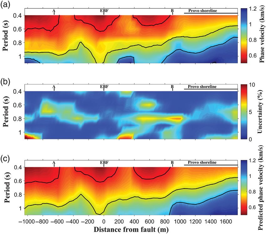
In this study, we use data
                                                                                                                           from a temporary linear nodal
                                                                                                                           array that was deployed across
                                                                                                                           1700 South Street in SLC. The
                                                                                                                           array cut across both the EBF
                                                                                                                           and the Provo shoreline
                                                                                                                           (Fig. 1), one of the major pale-
                                                                                                                           oshorelines of Lake Bonneville
                                                                                                                           (Oviatt, 2015). First, we com-
                                                                                                                           pute the cross-correlation
                                                                                                                           functions and use vertical–ver-
                                                                                                                           tical cross correlations to
                                                                                                                           extract Rayleigh waves propa-
                                                                                                                           gating along the line. A chal-
                                                                                                                           lenge in our analysis is the
                                                                                                                           presence of non-diffusive noise
                                                                                                                           in the ambient wavefield, likely
                                                                                                                           relative to urban activities. To
                  Figure 1. Street map of Salt Lake City (SLC) along 1700 South Street, showing station locations
                  (black triangles) of the temporary network. The surface trace of the East Bench fault (EBF) of the       enhance the signal and mea-
                  Wasatch fault system is shown with black solid lines (McKean, 2018; McDonald et al., 2020). The          sure phase velocities across
                  retrogressive phases of the Provo shoreline are shown with dotted lines (McKean, 2018). The              the linear array, we use the
                  upside-down triangle shows the virtual source station location used in the record sections of            double-beamforming method
                  Figure 2. Few major streets mentioned in the Data and Methods section are identified. Inset plot:        developed by Wang et al.
                  Map of western US where the location of Salt Lake City is indicated by a diamond.
                                                                                                                           (2019a,b), which has been suc-
                                                                                                                           cessfully applied to both
                                                                                                                           regional (Cascadia; Wang et al.,
                  damaging earthquake in the next 50 yr (Petersen et al., 2020),         2019a) and local scales (San Jacinto fault; Wang et al., 2019b).
                  the region represents some of the highest risk potential in the        In this study, we apply the method to study the shallow struc-
                  conterminous United States. The overall basin structure has            ture and simultaneously test its performance in an inland
                  long been constrained by geologic mapping (Gilbert, 1890)              urban environment. After we measure period-dependent phase
                  and borehole data (Kowalewska and Cohen, 1998), including              velocities, we invert the dispersion curve at each location for a
                  three major paleoshorelines of Lake Bonneville (Oviatt, 2015).         1D V S model using the weighted least-squares approach
                  The mechanical properties are less defined (Magistrale et al.,         described by Herrmann (2013). Finally, we combine all 1D
                  2009), because the sediments are prone to highly variable              V S models to produce a 2D V S model across the array.
                  amplification during earthquake shaking (Tinsley et al., 1991).
                      The fault system that contributes most to the seismic poten-       Data and Methods
                  tial in the area is the north–south-striking Wasatch fault sys-        A network of 32 nodal stations was deployed along 1700 South
                  tem (WFS). The WFS comprises 10 segments with total length             Street in SLC from 8 February to 12 March 2018 (station loca-
                  of more than 350 km, and is the largest normal fault in North          tions shown in Fig. 1; Lin, 2018). The linear array had an
                  America as part of the intermountain seismic belt, which               ∼2:9 km aperture and spanned from 700 East to 1900 East
                  bounds the eastern edge of the Basin and Range Province.               Street. The availability of deployment locations—primarily
                  Recent acquisition and analysis of light detection and ranging         local volunteer homeowners—resulted in some irregularity
                  data (McDonald et al., 2020) provide newly mapped fault                in station spacing with variation from ∼10 to ∼100 m.
                  scarps across the WFS segments and extends the surface traces
                  of known faults. Paleoseismic studies of the WFS (DuRoss et al.,       Noise cross correlations
                  2016) have identified six events with M > 6 in the last 5000 yr.       We compute ambient-noise cross correlations following Wang
                  The East Bench fault (EBF; surface mapping by McKean 2018;             et al. (2019a). Examples of the vertical–vertical (Z − Z) cross-
                  McDonald et al., 2020) is a subsystem of the Salt Lake segment         correlation record sections between a common station (virtual
                  of the WFS expressed as a series of en echelon west-dipping            source) close to the array center and all other receiver stations
                  faults that cross the SLC metropolitan area. Active-source seis-       across the array are shown in Figure 2, band-passed near 0.9 s
                  mic surveys in the area (Liberty et al., 2018a) have identified        (Fig. 2a) and 0.4 s (Fig. 2b). The observed Rayleigh-wave signal
                  the shallow expression of fault traces and relates velocity struc-     moveout is asymmetric, indicating stronger seismic energy
                  ture to the hydrostratigraphy of the area.                             propagating to the east. Besides the primary Rayleigh-wave

                  2       Seismological Research Letters                                                               www.srl-online.org   •   Volume XX   •   Number XX   •   – 2021

Downloaded from http://pubs.geoscienceworld.org/ssa/srl/article-pdf/doi/10.1785/0220200404/5246566/srl-2020404.1.pdf
by FanChi.Lin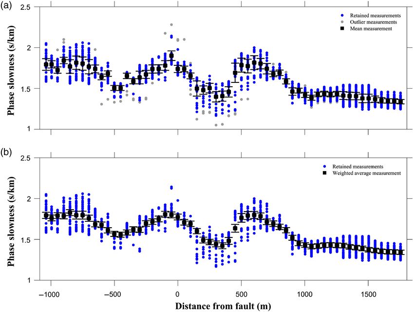
because of the limited array
                                                                                                                              aperture and hence the number
                                                                                                                              of beam pairs passing the selec-
                                                                                                                              tion criterion. The application
                                                                                                                              of this distance criterion can
                                                                                                                              still result in including individ-
                                                                                                                              ual station pairs with distance
                                                                                                                              smaller than 1 or 1.5 wave-
                                                                                                                              lengths, but we see no obvious
                                                                                                                              disturbance to the observed
                                                                                                                              Rayleigh-wave moveout when
                                                                                                                              including those short-distance
                                                                                                                              pairs. Following Wang et al.
                                                                                                                              (2019a), we assume planar
                                                                                                                              wavefront geometry and no
                                                                                                                              off-great-circle propagation.
                                                                                                                                  For each source–receiver
                                                                                                                              beam pair, we first cut and taper
                                                                                                                              the cross-correlation wave-
                                                                                                                              forms based on an empirically
                                                                                                                              determined period-dependent
                                                                                                                              maximum group              velocity
              Figure 2. Vertical–vertical cross-correlation functions between a virtual source station (gray reversed         (0:5–1:1 km=s).         Following
              triangle in Fig. 1) and all the array receivers, band-passed (a) near 0.9 s and (b) near 0.4 s. Solid line
                                                                                                                              Wang et al. (2019b), we then
              depicts a reference velocity line (1 km=s). Rayleigh-wave signal moveout is observed in the record
              sections with the dominant energy propagating toward the east. The color version of this figure is              shift and stack the waveforms
              available only in the electronic edition.                                                                       in the frequency domain
                                                                                                                              (Fig. 3a) using different source
                                                                                                                              (us ) and receiver (ur ) phase
                                                                                                                              slowness combinations, ranging
              signals, secondary signals are also observed especially at                   from 0.4 to 5 s=km. We measure the phase slowness on both
              shorter periods (Fig. 2b), likely due to the presence of persistent          source and receiver sides using a two-step grid search (coarse
              noise sources or active scatterers (Ma et al., 2013) in the vicin-           and finer grid, Wang et al., 2019b) based on the maximum
              ity of the study area. Although determining the nature of these              amplitude of the stacked waveform (beampower; example
              secondary signals is out of the scope of our current study,                  shown in Fig. 3b). To ensure that the grid search is picking
              future 2D dense array deployment in the area would allow                     the energy packet corresponding to the fundamental mode
              us to study the radiation pattern in detail and determine if                 Rayleigh-wave signal, we require the dispersion measurements
              the phase is fault-zone related.                                             to be continuous across different periods. We first determine the
                                                                                           phase slowness at periods longer than 0.9 s in which signals are
              Double-beamforming tomography                                                clean and simple. Starting at 0.9 s, we then use the slowness from
              To enhance the coherent Rayleigh-wave signals and measure                    the period immediately above as the reference slowness. Only
              phase velocities, we follow Wang et al. (2019a,b) and perform                source and receiver slowness measurements within 25% of their
              double beamforming. We form source and receiver beams                        corresponding reference slowness are accepted.
              across the array with a fixed 250 m beam width and 50 m beam                     After performing the grid search for all source and receiver
              center spacing. The beam width was chosen here to be large                   beam pairs across the array, the phase slowness at each location
              enough to include a sufficient number of stations (at least three            (i.e., each beam center) is determined by the mean of measure-
              stations in both the source and receiver beams). The beam                    ments at that location with different source-receiver beam com-
              width also intrinsically controls the lateral smoothing applied              binations. Measurements outside of two standard deviations
              by the method. We adopt a less strict far-field criterion to                 (st.dev.) are considered as outliers and removed. The uncertainty
              remove all beam pairs with distance between the source and                   for each location is computed as the st.dev. of the mean divided
              the receiver beam center smaller than either 1 or 1.5 wave-                  by the square root of independent measurements (Fig. 4a),
              lengths for periods between 1.1–0.7 and 0.6–0.4 s, respectively.             defined as the number of nonoverlapping beams (Wang et al.,
              Here, we use a 1 km=s reference velocity to estimate the wave-               2019a). To account for potential systematic biases due to an
              length. The slightly looser criterion for longer periods is                  uneven source distribution, we set the minimum uncertainty

              Volume XX        •   Number XX          •   – 2021      •   www.srl-online.org                               Seismological Research Letters      3

Downloaded from http://pubs.geoscienceworld.org/ssa/srl/article-pdf/doi/10.1785/0220200404/5246566/srl-2020404.1.pdf
by FanChi.Lin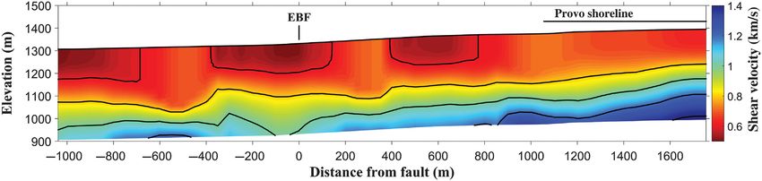
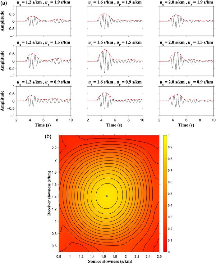
Figure 3. Example of the waveform shift and stacking procedure                                  indicate the envelope function of each stacked waveform.
                  and the 2D grid search for a beam pair at 0.5 s, in which the                                   (b) Beampower plot with varying source and receiver slowness.
                  source beam center is located at −0:6 km and the receiver beam                                  The black cross denotes the location of maximum beam
                  center is located at 1.25 km along the linear array (Fig. 2).                                   amplitude. Iso-amplitude contours are plotted as black lines
                  (a) Stacked waveforms after shifting using different source (us )                               using 0.05 interval. The color version of this figure is available
                  and receiver (ur ) phase slowness combinations. Dashed lines                                    only in the electronic edition.

                  4       Seismological Research Letters                                                               www.srl-online.org   •   Volume XX   •   Number XX   •   – 2021

Downloaded from http://pubs.geoscienceworld.org/ssa/srl/article-pdf/doi/10.1785/0220200404/5246566/srl-2020404.1.pdf
by FanChi.Lin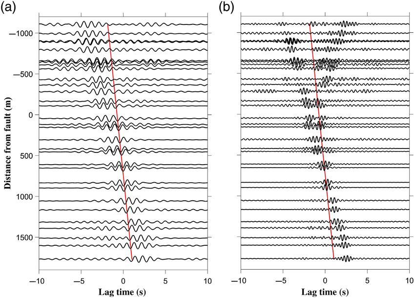
as 2% of the mean. In addition, we perform signal-to-noise ratio                                Figure 4. Phase slowness profiles for 0.5 s period. Phase slowness
              (SNR; Lin et al., 2009) calculations based on the stacked wave-                                 measurements not satisfying the SNR criterion are not shown.
              form and remove spurious measurements with SNR smaller                                          (a) Profile before smoothing and (b) profile after smoothing. The
                                                                                                              color version of this figure is available only in the electronic
              than 5. We define SNR as the peak-stacked waveform amplitude
                                                                                                              edition.
              within the signal window (velocity between 0:3 km=s and an
              empirically determined period-dependent maximum velocity
              between 0.5 and 1:1 km=s) divided by the root mean square
              of the noise window (20 s following the signal window).                                         The anomaly is wider at shorter periods and narrower at longer
              Considering the irregular station spacing and the significant                                   periods (0.8–1.1 s) potentially related to the depth-dependent
              beam overlap, we further smooth the phase slowness profile                                      fault-zone damage structure.
              for each period. The smoothed phase slowness and uncertainty
              at each location is computed as the weighted average of the three                               Shear-velocity inversion
              neighboring points (the three locations are 50 m apart) and the                                 To invert for a 2D V S model across the nodal array, we first
              standard error of the weighted average, respectively (Fig. 4b).                                 extract the Rayleigh-wave phase velocity dispersion curve at
              The phase slowness and their uncertainties for all periods are                                  each location across the profile. Then, we invert each
              combined and converted into phase velocity (Fig. 5a) and uncer-                                 dispersion curve independently using the iterative weighted
              tainty (Fig. 5b) profiles before shear-velocity inversions are per-                             least-squares algorithm of Herrmann (2013) to obtain a 1D
              formed. The overall slower phase velocities to the west and faster                              V S model. Following Wang et al. (2019b), we use a homo-
              phase velocities to the east likely reflect the thickening of sedi-                             geneous starting model with fixed V P =V S ratio equal to
              ments toward the center of the basin. On a smaller scale, a local-                              1.75 and an empirical density calculated from V P using the
              ized slow anomaly is observed near the surface trace of the EBF.                                relationship of Brocher (2005). Based on the geological setting

              Volume XX        •   Number XX          •   – 2021      •   www.srl-online.org                                                 Seismological Research Letters   5

Downloaded from http://pubs.geoscienceworld.org/ssa/srl/article-pdf/doi/10.1785/0220200404/5246566/srl-2020404.1.pdf
by FanChi.Lin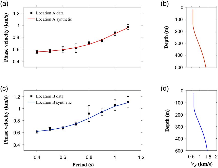
Results and
                                                                                                                                                     Discussion
                                                                                                                            The 2D shear-velocity model
                                                                                                                            (Fig. 8) exhibits similar spatial
                                                                                                                            patterns to the phase-velocity
                                                                                                                            map (Fig. 5a). The overall
                                                                                                                            trend in the V S profile is
                                                                                                                            decreasing velocity to the west
                                                                                                                            likely corresponding to sedi-
                                                                                                                            mentary thickening toward the
                                                                                                                            center of the basin (Radkins
                                                                                                                            et al., 1989; Hill et al., 1990).
                                                                                                                            The decreasing velocity may
                                                                                                                            also represent changes in the
                                                                                                                            overall composition of the
                                                                                                                            shallow lacustrine deposits,
                                                                                                                            which transition from younger
                                                                                                                            and softer clay, silt, and fine
                                                                                                                            sand in the west to older and
                                                                                                                            mechanically stronger sand
                                                                                                                            and gravel toward the east
                                                                                                                            (McDonald and Ashland,
                                                                                                                            2008). The highest velocities
                                                                                                                            (>1:2 km=s) in the model
                                                                                                                            observed at depth in the east
                                                                                                                            end of our model potentially
                                                                                                                            mark the transition between
                  Figure 5. (a) Phase-velocity map, (b) uncertainty map, and (c) predicted phase-velocity map cal-
                  culated from the inverted 2D V S model. Phase-velocity contours are separated by 200 m=s. The             shallow          unconsolidated
                  two example locations (A and B) used in Figures 6 and 7 are also denoted.                                 Quaternary sediments and
                                                                                                                            deeper Tertiary strata, com-
                                                                                                                            prised of volcanic and plutonic
                                                                                                                            rocks (Liberty et al., 2018b).
                  in the area, we impose a monotonically increase constraint to         The basin bedrock formations with shear velocities greater
                  the inverted 1D shear velocity models. We allow the inversion         than 3 km=s suggested by previous geophysical studies in the
                  to iterate up to 80 times to get the final 1D V S model, but stop     area (Bashore, 1982; Hill et al., 1990; Mabey, 1992; Magistrale
                  the iteration when the chi-square misfit does not improve by          et al., 2009) are likely below our maximum resolved depth; a
                  more than 1% compared to the previous iteration. On average,          future study with a larger array aperture is needed to constrain
                  the inversion stopped after ∼18 iterations.                           the deeper basin structure.
                      Examples of local dispersion curves and their inverted V S            The EBF is expressed in the period-dependent phase velocity
                  models are shown in Figure 6. The shear-velocity model for            (Fig. 6) and final V S profiles (Fig. 8) as a narrow asymmetric
                  location A (Fig. 6a, −0:55 km distance) is generally slower com-      low-velocity zone. Large-scale seismogenic faults are well known
                  pared to location B (Fig. 6c, 0.9 km distance). This is somewhat      to produce low velocities in their vicinity by breaking surround-
                  expected as location B is closer to the eastern basin edges and       ing rock during coseismic shaking (e.g., Ben-Zion and Sammis,
                  hence has thinner soft sediment. The observed phase velocity          2003); these features are termed “damage zones” and are typi-
                  dispersion curves in general can be fitted well by the model pre-     cally on the order of tens to hundreds of meters wide depending
                  dicted dispersion curves in which discrepancies are mostly            on the size of the largest earthquakes (Faulkner et al., 2011),
                  smaller than the estimated measurement uncertainties. We only         depth of the seismogenic zone (Ampuero and Mao, 2017),
                  consider the top 400 m of the inverted models robust consid-          cumulative fault slip (Sagy et al., 2007; Perrin et al., 2016), and
                  ering the overall depth sensitivity of our measurements (Fig. 7).     local rheology (e.g., Finzi et al., 2009; Molli et al., 2010; Thakur
                  We combine all 1D V S models across the profile to create a 2D        et al., 2020). In addition to the main mapped trace of the EBF,
                  V S model (Fig. 8). The predicted phase-velocity profile (Fig. 5c)    there are two other similar low-velocity zones (−1000 to −600 m
                  closely resembles the observed profile (Fig. 5a) with only notice-    and 400 to 800 m relative to EBF), which likely correspond to
                  able differences where uncertainties are high.                        other strands within the Wasatch fault zone; large-scale normal

                  6       Seismological Research Letters                                                               www.srl-online.org   •   Volume XX   •   Number XX   •   – 2021

Downloaded from http://pubs.geoscienceworld.org/ssa/srl/article-pdf/doi/10.1785/0220200404/5246566/srl-2020404.1.pdf
by FanChi.Lin
Hamiel, 2007). The main trace
of the EBF observed here
(Fig. 8) narrows with depth
from ∼600 m width at the sur-
face to ∼300 m width at the
bottom of the resolved profile.
The inferred damage zone is
asymmetric with respect to
the surface trace of the fault,
with more and higher intensity
damage in the hanging wall.
This pattern is expected for
normal faults and has previ-
ously been observed both geo-
logically (Flodin and Aydin,
2004; Berg and Skar, 2005)
and in numerical simulations
of dipping faults (Xu et al.,
2015). Because of the compli-
cated damage pattern and the
limited resolution of our tomo-
graphic image, it is difficult to
constrain the precise dip of
Figure 6. (a) Comparison between measured and synthetic dispersion curves at −0:65 km from EBF. the EBF and other subsidiary
(b) The inverted 1D V S model at −0:65 km. Panels (c,d) are same as panels (a,b) but at 0.9 km from strands from our result.
EBF. Error bars demonstrate uncertainties times 2. The color version of this figure is available only in However, the central portion
the electronic edition. of the damage zone is either
vertical or dipping slightly to
the west. If this is the case, it
is further support for a listric
faults are expected to branch into “flower structures” at shallow structure to the Wasatch fault zone (Mohapatra and Johnson,
depths due to the reduced normal stress (e.g., Twiss et al., 1992; 1998; Pang et al., 2020), listric structure to normal faults more
chapter 5). Previous active-source imaging in the same area generally (Wernicke, 1981; Davison 1986; Bose and Mitra,
resolved 11 fault strands across a 4.5 km linear array, only 2010), and is in line with free-surface orthogonality expectations
one of which was mapped at the surface (Liberty et al., from Andersonian faulting theory (Leung and Su, 1996).
2018b). We acknowledge that the observed localized low-veloc- The Provo shoreline is observed as a sharply bounded high-
ity zones can also be related to other factors (Wang, 2001), velocity region in the east within our 2D V S model (Fig. 8) with
including differences in sediment compaction rate and lithology much higher velocity at all resolved depths (particularly at
(e.g., Olig et al., 1996), layering-induced anisotropy (e.g., Behera depth). Because of this relatively sharp lateral boundary, which
et al., 2011), and increased porosity, pore-fluid saturation (e.g., persists to at least 400 m depth, we interpret this boundary as an
Shimeld et al., 2016). In addition, the low-velocity anomalies additional fault strand related to the EBF or Wasatch fault zone
may represent remnant liquefaction areas from past earthquakes more generally. Previously imaged non-fault shoreline bounda-
(e.g., Liberty et al., 2018a), and also be affected by interbedded ries in SLC have gradually thickened sediments westward from
smaller-scale structures such as colluvial wedges (e.g., the shoreline (Liberty et al., 2018b). A recent geodetic study (Hu
Buddensiek et al., 2008) with increasing thickness proportional et al., 2018) indicates that the EBF is also hydrological boundary
to past earthquake magnitude (e.g., Morey and Schuster, 1999). controlling surface deformation in the area.
Additional ground truth information (e.g., drilling cores) will be
required to distinguish these interpretations. Conclusions
The increasing normal stress with depth also leads to a nar- We present new results of noise-based shallow imaging in Salt
rower damage zone with depth (e.g., Allam and Ben-Zion, Lake Valley near the vicinity of the EBF using a dense linear
2012), either due to inhibited mode I fracture growth (e.g., array. We enhanced our noise cross-correlation signals and mea-
Prudencio and Van Sint Jan, 2007) or due to enhanced rock sured Rayleigh-wave phase velocities between 0.4 and 1.1 s
healing with increasing temperature (Lyakhovsky and Ya period across the array using the double beamforming method
Volume XX • Number XX • – 2021 • www.srl-online.org Seismological Research Letters 7
Downloaded from http://pubs.geoscienceworld.org/ssa/srl/article-pdf/doi/10.1785/0220200404/5246566/srl-2020404.1.pdf
by FanChi.Linnarrower with depth. The reso-
lution achieved in this study
enabled the imaging of this
low-velocity fault-zone struc-
ture for the first time, because
its spatial extent is smaller than
the resolution limit of previous
studies (e.g., Hill et al., 1990;
Magistrale et al., 2009). Our
results, along with other recent
studies (Liberty et al., 2018a;
McDonald et al., 2020; Pang
et al., 2020), indicate that the
fine-scale structure of the WFS
is a complicated series of fault
strands and their associated
damage. The success of this
study motivates future work in
the area to better understand
the structure and the seismic
hazard associated with the
WFS. The deployment of a net-
work with wider aperture and in
2D is needed to study the WFS
at greater depth, constrain its
Figure 7. V S sensitivity kernels for Rayleigh-wave phase velocity at 0.5, 0.7, and 1 s periods at two
lateral variation, and better
example locations. (a) −0:65 km and at (b) 0.9 km from EBF. understand the SLC urban noise
characteristics.
(Wang et al., 2019). Despite the less known and potentially com- Data and Resources
Seismic data from this network (DOI: 10.7914/SN/9H_2018) will be
plex noise wavefield associated with the inland metropolis, the
available to download from Incorporated Research Institutions for
observed phase velocity profile and 2D V S model constructed
Seismology (IRIS). Resources used for maps are available from the
between the surface and 400 m depth are consistent with the Utah Automated Geographic Reference Center (AGRC) (https://
geologic and the geotectonic models of the area. This indicates gis.utah.gov/) and the Utah Geological Survey (UGS). The surface
the ability of the method to produce reliable shallow crustal wave inversion tool used in this study is part of “Computer
images even in an urban environment far away from the ocean Programs in Seismology” (Herrmann, 2013) and available from
microseism. We provide new constrains on the shallow struc- http://www.eas.slu.edu/eqc/eqccps.html. All websites were last
ture of the EBF, which has an ∼400 m damage zone that gets accessed in October 2020.
Figure 8. 2D shear-velocity model constructed by piece-wise by 200 m=s.
continuous 1D inversions. Shear-velocity contours are separated
8 Seismological Research Letters www.srl-online.org • Volume XX • Number XX • – 2021
Downloaded from http://pubs.geoscienceworld.org/ssa/srl/article-pdf/doi/10.1785/0220200404/5246566/srl-2020404.1.pdf
by FanChi.LinDeclaration of Competing Interests Brocher, T. M. (2005). Empirical relations between elastic wavespeeds
The authors acknowledge there are no conflicts of interest and density in the Earth's crust, Bull. Seismol. Soc. Am. 95, no. 6,
recorded. 2081–2092, doi: 10.1785/0120050077.
Buddensiek, M. L., J. Sheng, T. Crosby, G. T. Schuster, R. L. Bruhn,
and R. He (2008). Colluvial wedge imaging using traveltime and
Acknowledgments waveform tomography along the Wasatch fault near Mapleton,
The authors thank Dylan Mikesell and an anonymous reviewer for
Utah, Geophys. J. Int. 172, no. 2, 686–697.
improving the context of the article. The authors thank Elizabeth
Castellanos, J. C., R. W. Clayton, and A. Juarez (2020). Using a time-based
Berg, Sin-Mei Wu, Jamie Farrell, and Jim Pechmann for constructive
subarray method to extract and invert noise-derived body waves at
discussions through this study. The authors thank Kevin Mendoza,
Long Beach, California, J. Geophys. Res. 125, no. 5, e2019JB018855.
Monique Holt, Elizabeth Berg, Clay Woods, and the students of the
Clayton, R. W. (2020). Imaging the subsurface with ambient noise auto-
University of Utah class “Seismic Imaging II” (Spring 2018) for their
correlations, Seismol. Res. Lett. 91, 930–935, doi: 10.1785/0220190272.
help during the deployment of the nodal stations and homeowners
Davison, I. (1986). Listric normal fault profiles: Calculation using
who volunteered to host nodal stations. This study was supported
bed-length balance and fault displacement, J. Struct. Geol. 8,
by the National Science Foundation Grant EAR 1753362. K. G. ac-
no. 2, 209–210.
knowledges a scholarship by the Alexander S. Onassis Foundation
De Ridder, S. A. L., and B. L. Biondi (2013). Daily reservoir-scale sub-
(Scholarship ID: F ZO 02-1/2018–2019).
surface monitoring using ambient seismic noise, Geophys. Res.
Lett. 40, no. 12, 2969–2974.
References DuRoss, C. B., S. F. Personius, A. J. Crone, S. S. Olig, M. D. Hylland,
Allam, A. A., and Y. Ben-Zion (2012). Seismic velocity structures W. R. Lund, and D. P. Schwartz (2016). Fault segmentation:
in the southern California plate-boundary environment from New concepts from the Wasatch fault zone, Utah, USA, J.
double-difference tomography, Geophys. J. Int. 190, no. 2, Geophys. Res. 121, no. 2, 1131–1157.
1181–1196. Faulkner, D. R., T. M. Mitchell, E. Jensen, and J. Cembrano (2011).
Ampuero, J. P., and X. Mao (2017). Upper limit on damage zone Scaling of fault damage zones with displacement and the implica-
thickness controlled by seismogenic depth, in Fault Zone tions for fault growth processes, J. Geophys. Res. 116, no. B5, doi:
Dynamic Processes: Evolution of Fault Properties during Seismic 10.1029/2010JB007788.
Rupture, Vol. 227, 243. Finzi, Y., E. H. Hearn, Y. Ben-Zion, and V. Lyakhovsky (2009).
Bashore, W. M. (1982). Upper crustal structure of the Salt Lake Valley Structural properties and deformation patterns of evolving
and the Wasatch fault from seismic modeling, M. S. Thesis, strike-slip faults: Numerical simulations incorporating damage
University of Utah, Salt Lake City, Utah, 95 pp. rheology, Pure Appl. Geophys. 166, nos. 10/11, 1537–1573.
Behera, L., P. Khare, and D. Sarkar (2011). Anisotropic P-wave veloc- Flodin, E., and A. Aydin (2004). Faults with asymmetric damage zones
ity analysis and seismic imaging in onshore Kutch sedimentary in sandstone, Valley of Fire State Park, southern Nevada, J. Struct.
basin of India, J. Appl. Geophys. 74, no. 4, 215–228. Geol. 26, no. 5, 983–988.
Ben-Zion, Y., and C. G. Sammis (2003). Characterization of fault Fu, H., C. He, B. Chen, Z. Yin, Z. Zhang, W. Zhang, T. Zhang, W. Xue,
zones, Pure Appl. Geophys. 160, nos. 3/4, 677–715. W. Liu, W. Yin, et al. (2017). 9-Pflops nonlinear earthquake sim-
Berg, E. M., F. C. Lin, A. Allam, V. Schulte-Pelkum, K. M. Ward, and ulation on Sunway Taihu Light: Enabling depiction of 18-Hz and
W. Shen (2020). Shear velocity model of Alaska via joint inversion 8-meter scenarios, Proc. of the International Conf. for High
of Rayleigh wave ellipticity, phase velocities, and receiver functions Performance Computing, Networking, Storage and Analysis, 1–12.
across the Alaska transportable array, J. Geophys. Res. 125, no. 2, Gilbert, G. K. (1890). Lake Bonneville, United States Geological
e2019JB018582, doi: 10.1029/2019JB018582. Survey, Monographs, Vol. 1, U.S. Government Printing Office,
Berg, S. S., and T. Skar (2005). Controls on damage zone asymmetry of Washington, DC, 438 pp.
a normal fault zone: Outcrop analyses of a segment of the Moab Graves, R. W., B. T. Aagaard, and K. W. Hudnut (2011). The
fault, SE Utah, J. Struct. Geol. 27, no. 10, 1803–1822, doi: 10.1016/ ShakeOut earthquake source and ground motion simulations,
j.jsg.2005.04.012. Earthq. Spectra 27, no. 2, 273–291.
Bose, S., and S. Mitra (2010). Analog modeling of divergent and Herrmann, R. B. (2013). Computer programs in seismology: An
convergent transfer zones in listric normal fault systems, AAPG evolving tool for instruction and research, Seismol. Res. Lett. 84,
Bulletin 94, no. 9, 1425–1452, doi: 10.1306/01051009164. no. 6, 1081–1088.
Bowden, D. C., V. C. Tsai, and F. C. Lin (2015). Site amplification, Hill, J., H. Benz, M. Murphy, and G. Schuster (1990). Propagation and
attenuation, and scattering from noise correlation amplitudes resonance of SHwaves in the Salt Lake Valley, Utah, Bull. Seismol.
across a dense array in Long Beach, CA, Geophys. Res. Lett. 42, Soc. Am. 80, no. 1, 23–42.
no. 5, 1360–1367, doi: 10.1002/2014GL062662. Hu, X., Z. Lu, and T. Wang (2018). Characterization of hydrogeo-
Brenguier, F., P. Kowalski, N. Ackerley, N. Nakata, P. Boué, M. logical properties in Salt Lake Valley, Utah, using InSAR, J.
Campillo, E. Larose, S. Rambaud, C. Pequegnat, T. Lecocq, et al. Geophys. Res. 123, no. 6, 1257–1271.
(2016). Toward 4D noise-based seismic probing of volcanoes: Johnson, L. R., and W. Silva (1981). The effects of unconsolidated
Perspectives from a large-N experiment on Piton de la Fournaise sediments upon the ground motion during local earthquakes,
Volcano, Seismol. Res. Lett. 87, no. 1, 15–25. Bull. Seismol. Soc. Am. 71, no. 1, 127–142.
Volume XX • Number XX • – 2021 • www.srl-online.org Seismological Research Letters 9
Downloaded from http://pubs.geoscienceworld.org/ssa/srl/article-pdf/doi/10.1785/0220200404/5246566/srl-2020404.1.pdf
by FanChi.LinKeifer, I., K. Dueker, and P. Chen (2019). Ambient Rayleigh wave field and Idaho, Utah Geol. Surv. Investig. Rept. 280, 23 pp., doi:
imaging of the critical zone in a weathered granite terrane, Earth 10.34191/RI-280.
Planet. Sci. Lett. 510, 198–208. McKean, A. P. (2018). Interim geologic map of the Sugar House quad-
Kowalewska, A., and A. S. Cohen (1998). Reconstruction of paleoen- rangle, Salt Lake County, Utah, Utah Geol. Surv. Open-File Rept.
vironments of the Great Salt Lake basin during the late Cenozoic, J. 687DM, 2 plates, scale 1:24,000, 28 pp.
Paleolimnol. 20, no. 4, 381–407. Mohapatra, G. K., and R. A. Johnson (1998). Localization of listric
Leung, A. Y. T., and R. K. L. Su (1996). Analytical solution for faults at thrust fault ramps beneath the Great Salt Lake Basin,
mode I crack orthogonal to free surface, Int. J. Fract. 76, no. 1, Utah: Evidence from seismic imaging and finite element modeling,
79–95. J. Geophys. Res. 103, no. B5, 10,047–10,063.
Li, G., H. Chen, F. Niu, Z. Guo, Y. Yang, and J. Xie (2016). Molli, G., G. Cortecci, L. Vaselli, G. Ottria, A. Cortopassi, E. Dinelli,
Measurement of Rayleigh wave ellipticity and its application to the M. Mussi, and M. Barbieri (2010). Fault zone structure and fluid–
joint inversion of high-resolution S wave velocity structure beneath rock interaction of a high angle normal fault in Carrara marble
northeast China, J. Geophys. Res. 121, no. 2, 864–880. (NW Tuscany, Italy), J. Struct. Geol. 32, no. 9, 1334–1348.
Li, J., F. C. Lin, A. Allam, Y. Ben-Zion, Z. Liu, and G. Schuster (2019). Mordret, A., P. Roux, P. Boué, and Y. Ben-Zion (2019). Shallow three-
Wave equation dispersion inversion of surface waves recorded on dimensional structure of the San Jacinto fault zone revealed from
irregular topography, Geophys. J. Int. 217, no. 1, 346–360. ambient noise imaging with a dense seismic array, Geophys. J. Int.
Liberty, L. M., J. S. Clair, and G. Gribler (2018a). Seismic land- 216, no. 2, 896–905.
streamer data reveal complex tectonic structures beneath Salt Morey, D., and G. T. Schuster (1999). Paleoseismicity of the Oquirrh
Lake City, SEG Technical Program Expanded Abstracts 2018, fault, Utah from shallow seismic tomography, Geophys. J. Int. 138,
Society of Exploration Geophysicists, 2662–2666. 25–35.
Liberty, L. M., J. S. Clair, and G. Gribler (2018b). Seismic profiling in Moschetti, M. P., S. Hartzell, L. Ramírez-Guzmán, A. D. Frankel, S. J.
downtown Salt Lake City: Mapping the Wasatch fault with seismic Angster, and W. J. Stephenson (2017). 3D ground-motion simu-
velocity and reflection methods from a land streamer, U.S. Geol. lations of M w 7 earthquakes on the Salt Lake City segment of the
Surv. Award G17AP00052 Rept., 47 pp., available at https:// Wasatch fault zone: Variability of long-period (T ≥ 1 s) ground
earthquake.usgs.gov/cfusion/external_grants/reports/ motions and sensitivity to kinematic rupture parameters, Bull.
G17AP00052.pdf (last accessed February 2021). Seismol. Soc. Am. 107, no. 4, 1704–1723.
Lin, F.-C. (2018). Salt Lake Linear Nodal Array 2018 [Data set], Nakata, N., P. Boué, F. Brenguier, P. Roux, V. Ferrazzini, and
International Federation of Digital Seismograph Networks, doi: M. Campillo (2016). Body and surface wave reconstruction from
10.7914/SN/9H_2018. seismic noise correlations between arrays at Piton de la Fournaise
Lin, F. C., D. Li, R. W. Clayton, and D. Hollis (2013). High-resolution volcano, Geophys. Res. Lett. 43, no. 3, 1047–1054.
3D shallow crustal structure in Long Beach, California: Nakata, N., J. P. Chang, J. F. Lawrence, and P. Boué (2015). Body wave
Application of ambient noise tomography on a dense seismic extraction and tomography at Long Beach, California, with ambi-
array, Geophysics 78, no. 4, Q45–Q56. ent-noise interferometry, J. Geophys. Res. 120, no. 2, 1159–1173.
Lin, F.-C., M. H. Ritzwoller, and R. Snieder (2009). Eikonal tomog- Olig, S. S., W. R. Lund, B. D. Black, and B. H. Mayes (1996).
raphy: Surface wave tomography by phase-front tracking across a Paleoseismic investigation of the Oquirrh fault zone, Tooele
regional broad-band seismic array, Geophys. J. Int., doi: 10.1111/ County, Utah, Utah Geol. Surv. Spec. Study 88, 22–54.
j.1365-246X.2009.04105.x. Oviatt, C. G. (2015). Chronology of Lake Bonneville, 30,000 to 10,000
Lobkis, O. I., and R. L. Weaver (2001). On the emergence of the yr BP, Quaternary Sci. Rev. 110, 166–171.
Green’s functionin the correlations of a diffuse field, J. Acoust. Pang, G., K. D. Koper, M. Mesimeri, K. L. Pankow, B. Baker, J. Farrell,
Soc. Am. 110, 3011–3017. J. Holt, J. M. Hale, P. Roberson, R. Burlacu, et al. (2020). Seismic
Lyakhovsky, V., and Y. Hamiel (2007). Damage evolution and fluid flow analysis of the 2020 Magna, Utah, earthquake sequence: Evidence
in poroelastic rock, Izvestiya Phys. Solid Earth 43, no. 1, 13–23. for a listric Wasatch fault, Geophys. Res. Lett. 47, no. 18,
Ma, Y., R. W. Clayton, V. C. Tsai, and Z. Zhan (2013). Locating a e2020GL089798.
scatterer in the active volcanic area of southern Peru from ambient Perrin, C., I. Manighetti, J. P. Ampuero, F. Cappa, and Y. Gaudemer
noise cross-correlation, Geophys. J. Int. 192, no. 3, 1332–1341. (2016). Location of largest earthquake slip and fast rupture con-
Mabey, D. R. (1992). Subsurface geology along the Wasatch front, in trolled by along-strike change in fault structural maturity due to
Assessment of Earthquake Hazards and Risk Along the Wasatch fault growth, J. Geophys. Res. 12, no. 5, 3666–3685.
Front, Utah, P. L. Goriand and W. W. Hays (Editors), U.S. Petersen, M. D., A. M. Shumway, P. M. Powers, C. S. Mueller, M. P.
Geol. Surv. Pro. Pap. 1500-A-J, C1–C16. Moschetti, A. D. Frankel, S. Rezaeian, D. E. McNamara, N. Luco,
Magistrale, H., J. Pechmann, and K. Olsen (2009). The Wasatch front, O. S. Boyd, et al. (2020). The 2018 update of the US National
Utah, community seismic velocity model, Seismol. Res. Lett. 80, 368. Seismic Hazard Model: Overview of model and implications,
McDonald, G. N., and F. X. Ashland (2008). Earthquake Site Earthq. Spectra 36, no. 1, 5–41.
Conditions in the Wasatch Front Corridor, Utah, Utah Prudencio, M., and M. V. S. Jan (2007). Strength and failure modes of
Geological Special Study, Vol. 125, 41 pp., 1 plate, scale 1:150,000. rock mass models with non-persistent joints, Int. J. Rock Mech.
McDonald, G. N., E. J. Kleber, A. I. Hiscock, S. E. K. Bennett, and S. D. Min. Sci. 44, no. 6, 890–902.
Bowman (2020). Fault trace mapping and surface-fault-rupture Radkins, H., M. Murphy, and G. Schuster (1989). Subsurface map and
special study zone delineation of the Wasatch fault zone, Utah seismic risk analysis of the Salt Lake Valley, Utah Geological and
10 Seismological Research Letters www.srl-online.org • Volume XX • Number XX • – 2021
Downloaded from http://pubs.geoscienceworld.org/ssa/srl/article-pdf/doi/10.1785/0220200404/5246566/srl-2020404.1.pdf
by FanChi.LinMineral Survey Report, Contract 5-24496, available at https:// Tinsley, J. C., K. W. King, D. A. Trumm, D. L. Carver, and R. Williams
ugspub.nr.utah.gov/publications/open_file_reports/OFR-152.pdf (1991). Geologic aspects of shear-wave velocity and relative ground
(last accessed February 2021). response in Salt Lake Valley, Utah, Proc. of the 27th Symposium on
Ranasinghe, N. R., L. L. Worthington, C. Jiang, B. Schmandt, T. S. Engineering Geology and Geotechnical Engineering, 25-1–25-9.
Finlay, S. L. Bilek, and R. C. Aster (2018). Upper-crustal shear- Twiss, R. J., R. J. Twiss, and E. M. Moores (1992). Structural Geology,
wave velocity structure of the south-central Rio Grande rift above R. J. Twiss and E. M. Moores (Editors), W. H. Freeman & Co., San
the Socorro magma body imaged with ambient noise by the Francisco, 532 pp., doi: 10.1002/gj.3350290408.
large-N Sevilleta seismic array, Seismol. Res. Lett. 89, no. 5, Wang, Y., A. Allam, and F.-C. Lin (2019b). Imaging the fault damage
1708–1719. zone of the San Jacinto fault near Anza with Ambient noise tomog-
Roux, P., L. Moreau, A. Lecointre, G. Hillers, M. Campillo, Y. Ben- raphy using a Dense Nodal array, Geophys. Res. Lett. 46, doi:
Zion, D. Zigone, and F. Vernon (2016). A methodological 10.1029/2019GL084835.
approach towards high-resolution surface wave imaging of the Wang, Y., F. C. Lin, B. Schmandt, and J. Farrell (2017). Ambient noise
San Jacinto fault zone using ambient-noise recordings at a spatially tomography across Mount St. Helens using a dense seismic array,
dense array, Geophys. J. Int. 206, no. 2, 980–992. J. Geophys. Res. 122, no. 6, 4492–4508.
Sagy, A., E. E. Brodsky, and G. J. Axen (2007). Evolution of fault-sur- Wang, Y., F. C. Lin, and K. M. Ward (2019a). Ambient noise tomog-
face roughness with slip, Geology 35, no. 3, 283–286. raphy across the Cascadia subduction zone using dense linear seis-
Shapiro, N. M., M. Campillo, L. Stehly, and M. H. Ritzwoller (2005). mic arrays and double beamforming, Geophys. J. Int. 217, no. 3,
High-resolution surface-wave tomography from ambient seismic 1668–1680.
noise, Science 307, no. 5715, 1615–1618. Wang, Z. (2001). Fundamentals of seismic rock physics, Geophysics
Shen, W., M. H. Ritzwoller, and V. Schulte-Pelkum (2013). A 3-D 66, no. 2, 398–412.
model of the crust and uppermost mantle beneath the central Wernicke, B. (1981). Low-angle normal faults in the Basin and Range
and western US by joint inversion of receiver functions and surface Province: Nappe tectonics in an extending orogeny, Nature 291,
wave dispersion, J. Geophys. Res. 118, no. 1, 262–276. no. 5817, 645–648.
Shimeld, J., Q. Li, D. Chian, N. Lebedeva-Ivanova, R. Jackson, D. Wu, S. M., F. C. Lin, J. Farrell, and A. Allam (2019). Imaging the deep
Mosher, and D. Hutchinson (2016). Seismic velocities within subsurface plumbing of Old Faithful geyser from low-frequency
the sedimentary succession of the Canada basin and southern hydrothermal tremor migration, Geophys. Res. Lett. 46, no. 13,
Alpha–Mendeleev ridge, Arctic Ocean: Evidence for accelerated 7315–7322.
porosity reduction? Geophys. J. Int. 204, no. 1, 1–20. Wu, S. M., F. C. Lin, J. Farrell, B. Shiro, L. Karlstrom, P. Okubo, and K.
Spica, Z., M. Perton, M. Calò, D. Legrand, F. Córdoba-Montiel, and A. Koper (2020). Spatiotemporal seismic structure variations associ-
Iglesias (2016). 3-D shear wave velocity model of Mexico and ated with the 2018 Kīlauea eruption based on temporary dense
south US: Bridging seismic networks with ambient noise cross- geophone arrays, Geophys. Res. Lett. 47, no. 9, e2019GL086668.
correlations (C 1 ) and correlation of coda of correlations (C 3 ), Wu, S. M., K. M. Ward, J. Farrell, F. C. Lin, M. Karplus, and R. B.
Geophys. J. Int. 206, no. 3, 1795–1813. Smith (2017). Anatomy of old faithful from subsurface seismic
Stokes, W. L. (1980). Geologic setting of Great Salt Lake, Great Salt imaging of the Yellowstone Upper Geyser Basin, Geophys. Res.
Lake 116, 54. Lett. 44, no. 20, 10–240.
Thakur, P., Y. Huang, and Y. Kaneko (2020). Effect of fault damage Xu, S., E. Fukuyama, Y. Ben-Zion, and J. P. Ampuero (2015). Dynamic
zones on long-term earthquake behavior on mature strike-slip rupture activation of backthrust fault branching, Tectonophysics 644,
faults, J. Geophys. Res. doi: 10.1029/2020JB019587. 161–183.
Thomas, A. M., Z. Spica, M. Bodmer, W. H. Schulz, and J. J. Roering
(2020). Using a dense seismic array to determine structure and site
effects of the two towers earthflow in northern California, Seismol. Manuscript received 29 October 2020
Res. Lett. 91, no. 2A, 913–920. Published online 10 March 2021
Volume XX • Number XX • – 2021 • www.srl-online.org Seismological Research Letters 11
Downloaded from http://pubs.geoscienceworld.org/ssa/srl/article-pdf/doi/10.1785/0220200404/5246566/srl-2020404.1.pdf
by FanChi.LinYou can also read