Photospheric plasma and magnetic field dynamics during the formation of solar AR 11190
←
→
Page content transcription
If your browser does not render page correctly, please read the page content below
Astronomy & Astrophysics manuscript no. ms                                                                                             c ESO 2019
                                              January 9, 2019

                                                   Photospheric plasma and magnetic field dynamics during the
                                                                   formation of solar AR 11190
                                                             J. I. Campos Rozo1, 2 , D. Utz1, 3 , S. Vargas Domínguez2 , A. Veronig1 , and T. Van Doorsselaere4

                                                    1
                                                        IGAM, Institute of Physics, University of Graz, Universitätsplatz 5, 8010 Graz, Austria
                                                        e-mail: jose.campos-rozo@uni-graz.at
                                                    2
                                                        Universidad Nacional de Colombia, Observatorio Astronómico Nacional, Ed. 413 Bogotá, Colombia
                                                        e-mail: svargasd@unal.edu.co
                                                    3
                                                        Instituto de Astrofísica de Andalucía IAA-CSIC, Es-18008 Granada, Spain
                                                        e-mail: dominik.utz@uni-graz.at
                                                    4
                                                        Centre for Mathematical Plasma Astrophysics, Department of Mathematics, KU Leuven, 3001 Leuven, Belgium
arXiv:1901.02437v1 [astro-ph.SR] 8 Jan 2019

                                                        e-mail: tom.vandoorsselaere@kuleuven.be
                                                   Received XXX ; accepted XXX

                                                                                                                 ABSTRACT

                                                   Context. The Sun features on its surface typical flow patterns called the granulation, mesogranulation, and supergranulation. These
                                                   patterns arise due to convective flows transporting energy from the interior of the Sun to its surface. The other well known elements
                                                   structuring the solar photosphere are magnetic fields arranged from single, isolated, small-scale flux tubes to large and extended
                                                   regions visible as sunspots and active regions.
                                                   Aims. In this paper we will shed light on the interaction between the convective flows in large-scale cells as well as the large-
                                                   scale magnetic fields in active regions, and investigate in detail the statistical distribution of flow velocities during the evolution and
                                                   formation of National Oceanic and Atmospheric Administration (NOAA) active region 11190.
                                                   Methods. To do so, we employed local correlation tracking methods on data obtained by the Solar Dynamics Observatory (SDO)
                                                   spacecraft in the continuum as well as on processed line-of-sight (LOS) magnetograms.
                                                   Results. We find that the flow fields in an active region can be modelled by a two-component distribution. One component is very
                                                   stable, follows a Rayleigh distribution, and can be assigned to the background flows, whilst the other component is variable in strength
                                                   and velocity range and can be attributed to the flux emergence visible both in the continuum maps as well as magnetograms. Generally,
                                                   the plasma flows, as seen by the distribution of the magnitude of the velocity, follow a Rayleigh distribution even through the time
                                                   of formation of active regions. However, at certain moments of large-scale fast flux emergence, a second component featuring higher
                                                   velocities is formed in the velocity magnitudes distribution.
                                                   Conclusions. The plasma flows are generally highly correlated to the motion of magnetic elements and vice versa except during the
                                                   times of fast magnetic flux emergence as observed by rising magnetic elements. At these times, the magnetic fields are found to move
                                                   faster than the corresponding plasma.
                                                   Key words. Photosphere – granulation – evolution – magnetic fields – sunspots

                                              1. Introduction                                                             tre, and fast outflows, they are called exploding granules (Title
                                                                                                                          et al. 1986, 1989). This happens during the final expansion at the
                                              High-resolution observations have shown that the solar photo-               last stage of their life. Such explosive granules are considered
                                              sphere is a non-uniform layer formed by different structures that           important in the context of the whole solar granulation evolution
                                              are constantly evolving at multiple spatial and temporal scales.            (Rösch 1961; Musman 1972; Namba & van Rijsbergen 1977).
                                              Some of these features form patterns, so-called convective cells,           Understanding the behaviour of the different granulation scales
                                              granules, “or in more colloquial terms, bubbles” (Hansen et al.             and granular evolution is important in order to obtain more real-
                                              2004). In the centre, these convective cells feature the emer-              istic quiet Sun models for the formation, as well as the evolution
                                              gence of hot plasma with vertical velocities of about 0.4 km s−1 ,          and decay of active regions (Roudier et al. 2003). The physical
                                              while towards their boundaries, the plasma motions become                   processes of the emergence of granular-scale magnetic fields are
                                              horizontal, moving to the intergranular lanes with velocities of            likely to be the same in the quiet Sun and active regions (Vargas
                                              0.25 km s−1 (Title et al. 1986). Diverse studies have shown how             Domínguez et al. 2012).
                                              granular cells can organize themselves in three main size scales:                Large-scale granules (mesogranules and supergranules) have
                                              granulation (∼ 1000 km; Bushby & Favier 2014), mesogranula-                 been associated to fast vertical upflows (Roudier et al. 2003;
                                              tion (5 − 10 Mm; November et al. 1981), and supergranulation                Guglielmino et al. 2010; Palacios et al. 2012; Verma et al. 2016).
                                              (> 20 Mm; Rieutord & Rincon 2010).                                          Moreover, exploding granules occur with certain preferences in
                                                  The evolution of the photospheric granulation pattern is de-            mesogranular regions (e.g. Massaguer & Zahn 1980; Title et al.
                                              termined by the expansion and the subsequent dissolution of                 1989) and during the emergence of magnetic field and its subse-
                                              granular cells (Rezaei et al. 2012; Palacios et al. 2012). When             quent accumulation within mesogranular borders (Simon et al.
                                              granules start to show the appearance of bright rings, a dark cen-          1988; Domínguez Cerdeña 2003; Ishikawa & Tsuneta 2011).
                                                                                                                                                                      Article number, page 1 of 15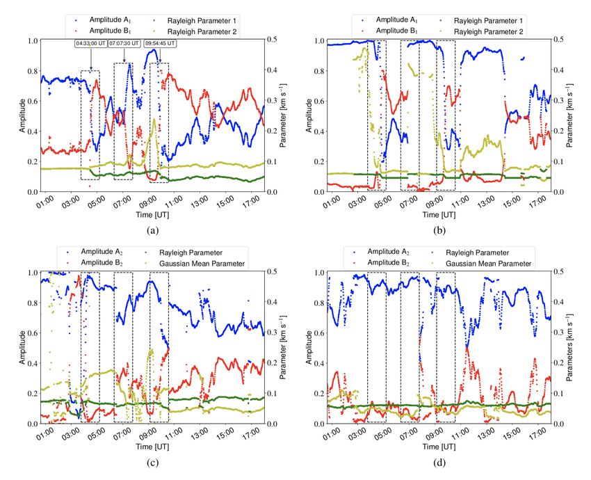
A&A proofs: manuscript no. ms

Fig. 1. Selected active region (AR) as observed on April 11, 2011 exhibits a complex configuration with sunspots harbouring partial penumbrae and
pores. The first row shows the time evolution of the continuum images for AR 11190 that displays a rapid evolution. The second row plots series of
LOS magnetograms for AR 11190 with positive and negative (white and black) magnetic polarities used to track the evolution of emergent positive
magnetic field. The solid box encloses the region of an initial positive magnetic emergence, while the dashed box outlines a second emergent cell
evolving faster and thus pushing and suppressing the first emergence. The colour bar in the first row displays the intensity values clipped between
45% and 95% of the image featuring the largest intensity, whereas the colour bar in the second row shows the LOS magnetic field maps clipped in
the range between −250 and +250 Gauss. A clearer understanding can be obtained by watching the full evolution of the active region in the movie
provided, which shows the magnetic field on a false colour table from −2500 G to +2500 G, and the continuum maps normalized over the average
of all the maximum (additional online supplement to the paper).1

In this paper, we focus on the behaviour of such large-scale gran-         nomena such as the shrinking-sun effect (Lisle & Toomre 2004)
ular cells within the region of interest (ROI) and at the time when        caused by large stationary flows. However, one can correct for
National Oceanic and Atmospheric Administration (NOAA) ac-                 these errors and thus such artefacts can successfully be removed
tive region 11190 is formed. Such detailed studies were not pos-           by subtracting the time average of the velocities from the flow
sible, due to the lack of highly resolved, long, and sufficiently          maps. Some authors (e.g. Yi et al. 1992; Molowny-Horas 1994;
stable time series for the detailed investigation of the forma-            Verma et al. 2013; Louis et al. 2015; Asensio Ramos et al. 2017)
tion of an active region over days on spatial scales down to the           have shown that in the worst cases the underestimations of ve-
granulation. With highly sophisticated space instruments like the          locities may amount to 20-30%.
SDO spacecraft (Solar Dynamics Observatory, see Pesnell et al.
2012), used in this study, we can follow the long temporal evolu-
tion necessary for the formation and dissolution of whole active           2. Data and pre-processing
regions.                                                                   In this study we use time series of imaging data showing the
     For the detailed flow investigations performed in this study,         formation and evolution of active region (AR) 11190. The data
we need to identify the proper surface motions. Several authors            were acquired by the Helioseismic and Magnetic Imager (HMI)
have studied these kinds of proper motions using different ap-             instrument (Hoeksema et al. 2014) on board the SDO space-
proaches (e.g. Hurlburt et al. 1995; Simon et al. 1995; Welsch             craft comprising continuum maps and line-of-sight (LOS) mag-
et al. 2004; Schuck 2006). Among the most widely applied meth-             netograms.
ods is the so-called local correlation tracking (LCT) technique.               The studied AR 11190 is shown in Fig. 1, and comprises the
LCT was employed for the calculation of proper motions of the              formation stage during the time interval for the whole 24 hours
solar granulation for the first time by November et al. (1986),            on April 11, 2011 in continuum as well as in LOS magnetic
and subsequently by November & Simon (1988). The algorithm                 field. The maps are acquired with a cadence of 45 seconds
is based on finding the best cross-correlation between two con-            and a pixel resolution of ∼ 0.504 arcsec (roughly 350 km) for
secutive images. It is well known that LCT can produce some                both observable quantities (continuum, LOS magnetic field).
errors due to the method itself when it measures the intensity             As these data come already prepared at level 1.5, no primary
changes as these changes can be related to plasma motions but              data reduction such as flat fielding and dark current correction is
also may reflect phase velocities (e.g. Roudier et al. 1999; Potts         necessary.
et al. 2003). In addition, LCT may produce errors through phe-
1
  A movie showing the full evolution can be found                     at      Figure 1 shows four different instances prior to the formation
https://github.com/Hypnus1803/PlotsSunspots/blob/                          of AR 11190 in continuum and LOS magnetic field images.
master/VideoPaper/CubeMag_20110411_hmicmap.mp4.                            The video linked to the web url mentioned above shows clearly
Article number, page 2 of 15
J. I. Campos Rozo et al.: Plasma and magnetic field dynamics during the formation of AR 11190
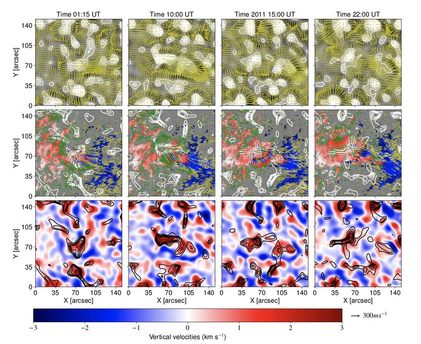
Fig. 2. Temporal evolution of the velocity fields within the ROI of AR 11190 at four different times computed by local correlation tracking
(LCT) analysis. Horizontal and vertical velocities are inferred from continuum maps as well as from LOS magnetic field maps. The top panel
shows the horizontal proper motions (calculated by LCT technique applied to the continuum maps) with the background image being the vertical
velocity map, and the contour lines representing positive vertical velocities with contour values of [0.5, 1., 1.5, 2., 3] km s−1 . The second row
displays the horizontal velocities of magnetic elements (calculated from LCT analysis over the LOS magnetograms) where the background image
represents the LOS magnetic field strength map and the contour lines are ranged as before. The red arrows show the motions of magnetic elements
with magnetic strengths greater than 50 Gauss, and the blue arrows display the average movements of negative magnetic elements with values
lower than -50 Gauss. The green arrows display horizontal behaviour for weak positive magnetic elements, whereas the yellow arrows display
the horizontal proper motions associated with weak negative magnetic field elements. The third row shows a comparison between the evolution
of vertical velocities obtained from the continuum data set and the evolution of positive vertical velocities obtained from the LOS magnetic field
data. The black arrow in the bottom right corner represents the length of a velocity vector featuring a magnitude of 300 m s−1 .
the emergence of the first magnetic bubble (Ortiz et al. 2014; Moreover, Fig. 1 (LOS maps) shows pre-existent positive
de la Cruz Rodríguez et al. 2015), and then a second even and negative magnetic field regions. When the first magnetic
faster and more powerful magnetic emergence starts to occur, bubble appears within the field of view (FOV), the positive and
lifting more positive magnetic flux to the surface and pushing negative magnetic elements further away from the site of emer-
the previously emerged flux to the right. The faster emergence gence (constituting in some way the background magnetic envi-
is seen even more clearly in the evolution of magnetograms ronment) do not change noticeably. At the same instant that the
compared to the observations in the continuum data. In this second magnetic bubble starts to emerge, it pushes the first emer-
LOS magnetogram, a solid box (see second row in Fig. 1) gence away from the location of newly emergent flux. Thus, soon
encloses an initial positive magnetic field emergence, which after, all the previously emerged magnetic elements are pushed
starts during the first hours of the day, whereas a dashed box in the same right direction towards the negative magnetic ele-
encloses the second magnetic emergence. The LOS maps dis- ments. These magnetic elements in turn start to accumulate at
played in the figure were clipped in the range [−250, 250] Gauss. certain locations, increase there in magnetic flux, and evolve for
Article number, page 3 of 15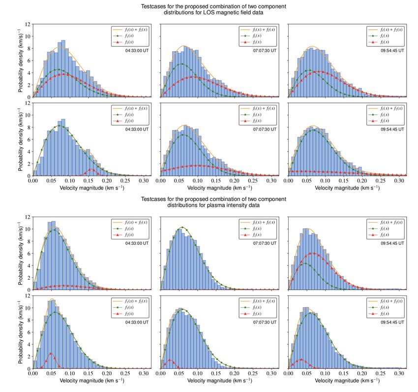
A&A proofs: manuscript no. ms

                                                                                              Fig. 3. Distribution
                                                                                                          q        of magnitudes of veloc-
                                                                                              ities (v = v2x + v2y ; speeds) for weak and
                                                                                              strong magnetic fields for the times shown
                                                                                              in Fig. 2. Red and blue colours (thick lines)
                                                                                              describe the velocity distributions for pos-
                                                                                              itive and negative magnetic fields greater
                                                                                              than 50 Gauss, whereas green and yellow
                                                                                              (thin lines) distributions represent the mo-
                                                                                              tions of the weaker magnetic elements. The
                                                                                              ranges for both the weak positive and neg-
                                                                                              ative field strengths are [10 < B < 50 &
                                                                                              −50 < B < −10] Gauss. Here, B is the
                                                                                              magnetic field strength as obtained from
                                                                                              the magnetograms. The solid lines repre-
                                                                                              sent the positive magnetic polarity, whereas
                                                                                              the dashed lines represent the negative mag-
                                                                                              netic fields.

                                                                                             Fig. 4. Distribution of speeds. The red
                                                                                             dashed line shows the distribution of v for
                                                                                             the proper motions, whereas the blue and
                                                                                             solid line shows the distribution of magnetic
                                                                                             elements motion. The scale factor σ is asso-
                                                                                             ciated with the mean velocity in this distri-
                                                                                             bution.

the first time into small magnetic pores that later on become the   a subsonic filtering with a phase-velocity threshold of 4 km s−1
fully evolved AR 11190.                                             was applied to subtract the solar 5-minutes oscillation (Novem-
    The software used for reducing HMI data (e.g. derotation,       ber et al. 1981; Title et al. 1989). Moreover, due to the Sun being
coaligment, and subsonic filtering procedures) was encoded in       a hot plasma sphere and the sunspot locations spreading along
the Python language making use of the solar physics library         different regions on the solar disc, flow map velocity compo-
named Sunpy (SunPy Community et al. 2015). A graphical user         nents were properly deprojected (see Vargas Dominguez 2009,
interface (GUI) has been developed to facilitate the detection      and references therein).
and application of the LCT method (see Campos Rozo & Var-
gas Dominguez 2014)2 . The ROI was chosen manually in such
a way as to centre on the location where the emergence of fast      3. Results
and highly notable large-scale granules is happening. The size of
the analyzed FOV is 15000 × 15000 . All images were aligned and     We focused on the formation and emergence of AR 11190, and
                                                                    investigated in detail the evolution and behaviour of the plasma
2
  The code can be found at https://github.com/Hypnus1803/           and magnetic field dynamics from horizontal and vertical ve-
FlowMapsGUI.                                                        locities for different time ranges. The LCT technique applied is
Article number, page 4 of 15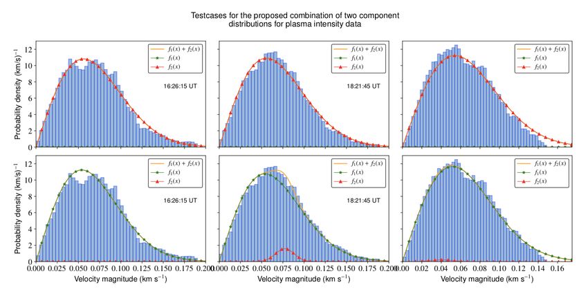
J. I. Campos Rozo et al.: Plasma and magnetic field dynamics during the formation of AR 11190

Fig. 5. Plots show three test cases for the proposed combination of two-component distributions for the continuum flow maps (lower set of panels)
as well as for the magnetic elements motions (upper set of panels). The first row in both six panel sets depicts the case of combining two Rayleigh
distributions for the total fit. They display the two independent Rayleigh components as well as the sum of the two components to form the whole
measured velocity distribution for three different times. The second row for each of them displays in the same way the case of the combination of
a Rayleigh background component with a variable Gaussian component. Times are in universal time (UT).

based on Eq. 1 proposed by November & Simon (1988),                        plasma physical properties. The LCT algorithm applied in this
                                                                           work (see Yi et al. 1992; Molowny-Horas 1994) was adapted
                        δ       δ
                 Z
                                                                           in Python to calculate the velocity fields using an apodization
Ct,t+τ (δδ, x) =  Jt ζ − Jt+τ ζ + W(x − ζ )∂ζζ ,                    (1)
                        2        2                                         window adjusted for the comparable size of the features to be
                                                                           tracked. Authors such as Palacios et al. (2012) have shown that
where Ct,t+τ (δδ, x) is a four-dimensional function depending on           the emergence of new magnetic flux as well as posterior AR for-
two consecutive images, the displacements between these im-                mation are associated with explosive mesogranules.
ages, and the localization of the apodization window W(x); and
Jt , Jt+τ are the intensity of the images at two consecutive time              For that reason we have chosen a full width at half maximum
steps t and t + τ. It is worth mentioning that the velocities es-          (FWHM) parameter of 12.5 arcsec (∼ 9 Mm) corresponding to
timated by LCT are not exclusively plasma motions but strictly             typical average sizes of ensembles of granules forming the meso-
speaking horizontal proper motions as the algorithm does not use           granular pattern, and a temporal averaging period of 2 hours
                                                                                                                     Article number, page 5 of 15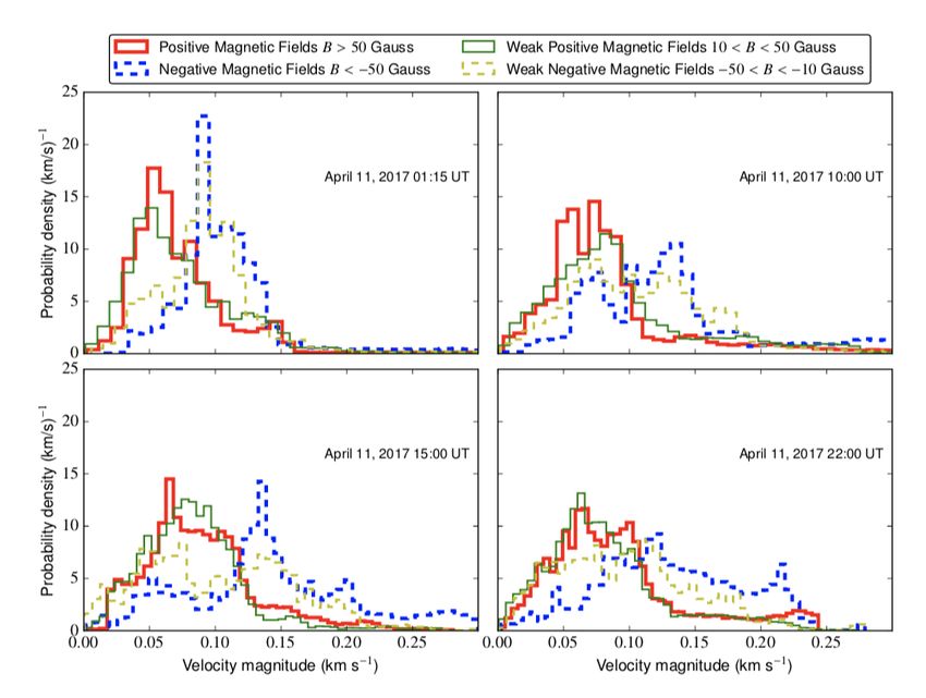
A&A proofs: manuscript no. ms

(average lifetimes for large-scale granulation patterns; see Hill      positive vertical velocities enclosing magnitudes of [0.5, 1., 1.5,
et al. 1984; Rast 2003). These 2 hours correspond to 160 frames        2., 3] km s−1 calculated from the continuum data set.
in the data set.3 Vertical velocities are computed by the diver-            The second row in Fig. 2 features plotted contours of the
gence from the horizontal velocities v x and vy obtained by the        vertical velocities calculated from the LOS magnetic field data
LCT algorithm via the idea of flux conservation (see November          using the same contour values mentioned before. This panel
& Simon 1988; Márquez et al. 2006; Vargas Dominguez 2009)              shows also the horizontal motions of positive and negative
leading to the expression                                              magnetic elements in the LOS maps. It is possible to identify the
                                                                       moment when the second magnetic emergence starts to appear
vz (v x , vy ) = hm ∇ · vh (v x , vy ),                         (2)    (row=2, column=2). This emergence shows fast motions but
                                                                       only associated with weak positive magnetic field elements that
where hm is a constant of proportionality representing the mass-       turn later into strong magnetic field elements.
flux scale height with a value of 150 ± 12 km (see November
et al. 1987; November 1989). The flow maps are then plotted                In order to compare the dynamics of plasma and magnetic
over these vertical velocities obtained from continuum maps as         elements, Fig. 2, third row, shows in the background the verti-
well as from magnetograms.                                             cal velocities from the continuum data set as well as overplotted
                                                                       contour lines representing the positive vertical velocities calcu-
3.1. Horizontal and vertical flow maps                                 lated from the LOS magnetic data cube. Although all vertical
                                                                       velocities calculated from magnetic LOS elements are linked to
The studied AR shows exploding mesogranules in locations               plasma vertical velocities, the best observational correlation is
where the formation of the active region, as seen by a complex         registered for the emergence located in 7000 × 7000 . Both flow
sunspot group, is initiated. There is a strong connection between      patterns seem to evolve at the same rate and look alike.
the appearance of these emergent large-scale granules and rapid            However, to have an even more robust and quantitative
vertical upflows emerging from the same region. Even when              overview of the ongoing and evolving flows, we will q   now have
AR 11190 does not show strong emergences in the continuum
maps, a strong emergence of positive magnetic field elements           a detailed look at the distribution of the magnitudes ( v2x + v2y ;
can be clearly observed in the magnetograms. Horizontal and            hereafter called speed) separated for the previously mentioned
vertical flow maps of proper motions as well as of magnetic field      strong and weak fields, as well as for the two polarities.
elements were calculated with the LCT algorithm to link the            The resulting distribution of speeds for the same four time in-
photospheric plasma dynamics with the magnetic field evolution.        stances (at the beginning of the first emergence, during the sec-
                                                                       ond emergence, after the second emergence, and to the end of
    Figure 2 shows the evolution of the magnetic flux and plasma       the evolution) can be seen in Fig. 3. At the beginning of the first
emergence during the formation of AR 11190 as well as the be-          emergence (left upper panel) one can see a separation of the pos-
haviour of the plasma and the movement of the magnetic ele-            itive and negative polarities.
ments as observed in the LOS magnetograms at four different            While the distributions for the positive magnetic field elements
time. The horizontal and vertical velocities are plotted in each       look more or less Rayleigh distributed (indicating a two dimen-
panel showing the behaviour and giving information about the           sional freely, i.e. randomly, outflowing region), the same distri-
proper motions of the plasma and the magnetic elements during          bution for the negative magnetic elements features the appear-
the appearance of AR 11190.                                            ance of a normal distribution, but offset from zero by a certain
The first panel displays the evolution and behaviour of the con-       constant velocity, indicating a movement leading to a separation
tinuum maps. The horizontal velocities are represented by the          for the two polarities, where the negative magnetic elements tend
arrows overplotted in the ROI, whereas the vertical velocities         to move towards the right side of the FOV. During and just after
are represented by the background image. These velocities re-          the second emergence (panels 2 and 3 in Fig. 3) the distribu-
veal several divergences at the following positions: (x00 , y00 ) =    tions seem to be truncated and merging at horizontal velocities
(70, 30), (30, 5), (70, 70), or (50, 130).                             of around 0.12 km s−1 . This behaviour can be explained by the
We focus now on the emergence centred on the position 7000 ×           idea that the created positive magnetic elements catch up with
7000 as it displays a comparably more rapid emergence of strong,       the negative elements towards the right side. After catching up,
as well as weak, positive magnetic field elements, as evidenced        these negative elements then hinder the positive ones in mov-
in the second row at the same location, which can be found at the      ing faster. Thus the positive distribution gets truncated at higher
other emergence sites. Although the other emergences indicate a        velocities while the distribution for negative elements becomes
certain correspondence of vertical motions between plasma and          truncated for low velocities as the positive elements push into the
the LOS magnetic elements, they do not display horizontal mo-          slowest negative ones thus either accelerating them to the same
tions of positive magnetic elements greater than 10 Gauss (lower       speed or annihilating them when they catch up. The last panel
limit used in the present work) emerging in those regions.             in Fig. 3 (lower right one) shows the evolved FOV where both
Before the appearance of the second emerging bubble, the mo-           kinds of magnetic elements seem to approach very similar dis-
tions of the magnetic elements follow the paths imposed by             tributions and thus move and evolve together again.
the plasma horizontal motions as well as the up- and down-             Figure 4 displays the speeds of the horizontal proper motions
flows. When the second magnetic emergence starts to appear,            (red dashed line) and the horizontal movements of magnetic el-
the proper motions seem to follow the new paths imposed by the         ements (blue and solid line; now regardless of their polarity and
new strong positive magnetic field elements, displaying a pre-         strength). The upper panels in Fig. 4 show a correspondence be-
ferred motion in the positive x-direction (see also additional on-     tween the plasma and magnetic field distributions, which means
line movies). In the first row of Fig. 2, the contour lines show       that both are moving following the same behaviour. As they are
                                                                       evolving (bottom panels), the velocity distribution of the mag-
 3
   We wish to remark that given UT times on the images always corre-   netic elements shows an increase in its mean value, whereas
spond to the first image of such 160 images containing subsets.        the mean velocity obtained from the proper motions appears to
Article number, page 6 of 15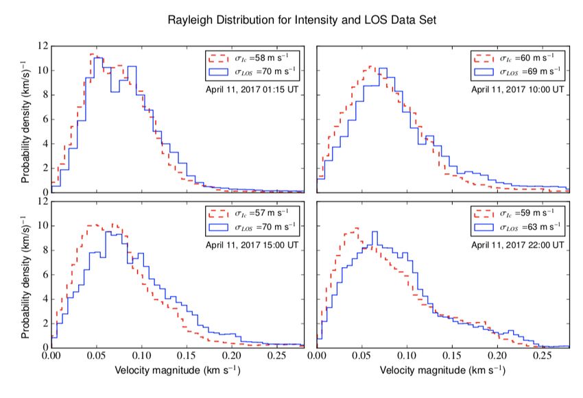
J. I. Campos Rozo et al.: Plasma and magnetic field dynamics during the formation of AR 11190

decrease in value most likely being suppressed by the stronger           and one Gaussian component (see Eq. 5):
magnetic fields. Due to the physical processes creating the flows,
                                                                         f (v, σR1 ) + f (v, σR2 ) =
the best description of the distribution of speeds is generally                              −v2                    −v2
given by a Rayleigh distribution (Eq. 3)4 ,                                        v                         v                             (4)
                                                                            A1 · 2 exp               + B1 ·      exp        ,
                                                                                 σ R1        2σ2R1          σ2R2      2σ2R2

             v       −v2                                               f (v, σR3 ) + f (v, µG , σG ) =
f (v, σ) =      exp         , v > 0,                              (3)              v         −v2         B2        −(v − µ )2
             σ2       2σ2                                                   A2 · 2 exp                +  √      exp
                                                                                                                              G
                                                                                                                                  .        (5)
                                                                                 σ R3         2σ2R3        2πσG          2σ 2
                                                                                                                            G
     where the scalar factor σ is associated with the mean velocity          In these equations σ represents either the previously intro-
of such a distribution (Hoffman et al. 1975). The mean velocity          duced scalar parameter of a Rayleigh distribution or the standard
for a quiet small region, using temporal averages of 2 hours, is         deviation in the case of the Gaussian. Constants A x and Bx are the
vInt = 72 ± 8.8 ms−1 for the continuum maps, whereas for LOS             amplitudes or weighting parameters for the two components of
magnetogram data the value amounts to vLOS = 54 ± 10.7 ms−1 .            the distribution with x = 1 representing the double Rayleigh dis-
However, when the mean velocity is calculated over the chosen            tribution and x = 2 corresponding to the Rayleigh and Gaussian
ROI, the horizontal proper motions obtained from the magnetic            combined distribution. Finally, µG represents the mean value of
elements data (vLOS = 65 ± 2.2 ms−1 ) appear to be slightly larger       the Gaussian distribution. By applying such a model, we would
than the continuum proper motions (vInt = 55 ± 2.5 ms−1 ). This          implicitly assume that the flux emergence leads in a part of the
difference can be explained by the second faster emergence of            FOV to a secondary Rayleigh distribution or a Gaussian one
magnetic field. During this emergence the plasma takes some              most likely featuring higher velocities than the background flow
time until it starts to feel the influence of these new magnetic         distribution.
fields that emerge faster than the first appearance and start to             Three test cases at different time instants of such two-
push the old magnetic elements. In the photosphere most of the           component modelling of the flows in the FOV of the flux emer-
plasma is, due to the comparably low temperatures, in a neu-             gence are shown in Fig. 5. The upper part of the figure shows
tral state. Thus, in the beginning of the flux emergence, only the       a set of six panels created from the LCT analysis of magne-
present ions will react immediately, while some time is needed to        tograms. The first row of these panels shows the combination of
transfer the momentum from the ions to the neutral gas. There-           two Rayleigh components while the lower row shows the com-
fore the proper motions linked to the continuum maps and their           bination of a Rayleigh component and the Gaussian distribution.
velocity distributions can lag behind the distributions of the mag-      The lower set of panels is arranged in the same way but created
netic elements. Besides, we have to have in mind that the forma-         from the LCT analysis of the continuum maps. These three cases
tion height for the continuum maps can be slightly different from        were chosen visually from Fig. 6a at times that showed remark-
the formation height of the magnetograms. The existence of a             able changes in the evolution of the depicted parameters. In these
strong concordance between both distributions, continuum and             three test cases it becomes clear that sometimes the combination
magnetic elements motions, is nevertheless evident even though           of two Rayleigh components fits better, while in other cases the
the magnetic elements move horizontally slightly faster than the         combination of a Rayleigh component with a Gaussian compo-
horizontal motions computed from continuum maps.                         nent gives a better fit.
                                                                             From these modelling efforts, we can learn that it is not
3.2. Distribution analysis                                               straightforward and clear whether the additional component
                                                                         should be of Rayleigh or of Gaussian type. For instance, for the
Figure 4 shows, for the velocity distribution of the magnetic field      speed histograms created from the continuum maps as depicted
elements, distinct enhancements variable in position as well as          in the first column, it is easy to observe that the combination
amplitude. Due to this behaviour, we introduce and consider              of a Rayleigh distribution with a Gaussian distribution fits bet-
a combined distribution model made up of two components.                 ter compared to the combination of two Rayleigh distributions.
While the major part of the histogram follows a Rayleigh dis-            This is also true for the distribution created by the LOS mag-
tribution (first component) representing undisturbed quiet back-         netic field data set. The middle column of distributions created
ground flows, the second component will be generally related to          from the magnetograms as well as continuum maps seem to be
the flux emergence process creating, for example, a tail of high         equally well fitted by both kinds of combined distributions, while
velocity measurements. In addition to the increased velocity tail,       the last column shows that the distributions would be better fit-
it is also possible that during the flux emergence a bifurcation of      ted by the two Rayleigh components combination. The second
the velocity distribution happens due to different velocity distri-      finding is that clearly the amplitude of the secondary component
butions for the two magnetic field polarities, meaning that one          is variable in position as well as in amplitude.
kind of magnetic element moves with a different characteristic               We do not wish to introduce a model with too many free
speed than the other. Thus the bumpy nature can be explained by          parameters and thus we will continue with these models that
the flux emergence process and/or a bifurcation of the underly-          only comprise the mentioned two components. However, to shed
ing velocity distributions for the two magnetic polarities. Due to       more light on the goodness of these combinations, we will now
the unknown nature of the second distribution, we will employ            investigate in more detail the temporal evolution of the param-
fitting tests with a combination of either two Rayleigh distribu-        eters of such two-component models. Later, we will then also
tions (see Eq. 4) or a combination of one Rayleigh component             study the goodness of the fit of the combined models to ascer-
                                                                         tain which one is more likely to represent the flows in the FOV
 4
   Mathematically, a Rayleigh distribution for the magnitude of a two-   during flux emergence events.
dimensional vector is formed when both vector components follow 0-           Figure 6 displays an example of how the fit parameters be-
centred normal distributions with equal σ (standard deviation), which    have during the time evolution on April 11, 2011. The left col-
is common for random walk processes (convective flows)                   umn shows the behaviour for the LOS magnetic field data set,
                                                                                                                   Article number, page 7 of 15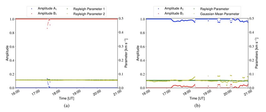
A&A proofs: manuscript no. ms

Fig. 6. Temporal evolution of the parameters associated with the proposed distributions in Eqs. 4 and 5. The first row shows the behaviour of the
parameters for the sum of two Rayleigh functions. The second row displays the time evolution for the combination of one Rayleigh function and
one Gaussian function. The temporal evolution followed by the amplitudes (dimensionless – left axis) is plotted with circle markers, whereas the
temporal evolution for the functional parameters are shown with star markers (right axis in km s−1 ). The blue and green markers are associated to
the first Rayleigh function component in both proposed distributions, whereas the red, and yellow markers represent the second component, which
is either a second Rayleigh function or a Gaussian function. The left side of the panels are calculated from the LOS magnetograms, whereas the
right side panels are obtained from the continuum maps. The dashed rectangles enclose the three time instants shown in Fig. 5.

whereas the right column gives the information about the proper           ters. Moreover, the amplitude B1 becomes larger than the ampli-
motions obtained from the continuum maps. Figures 6a and 6b               tude A1 giving more importance to the second component at this
present the parameters A1 , B1 , σR1 , and σR2 , calculated using a       moment of evolution. The second time shows a small enhance-
python least-square algorithm for the case of applying the sum of         ment of the Rayleigh parameter for the second component. How-
two Rayleigh distributions (Eq. 4) for the LOS data set, as well          ever, in this instance the amplitude A1 becomes greater than B1 .
as for the continuum data. Parameter σR1 is related to the back-          This change may be associated with the beginning of the second
ground velocity at those places of the ROI where the plasma or            magnetic emergence. The third and the strongest change in the
the magnetic elements are not affected by flux emergence. One             Rayleigh parameters related to the second distribution happens
can clearly observe in Fig. 6a the existence of three strong de-          at 09:54:45 UT. At this point the second magnetic emergence be-
viations at three different times (marked dashed rectangles, and          comes more active, associated with an increased number of pos-
their respective times) that affect all the parameters at the same        itive magnetic field elements. Figure 6b, which shows the evolu-
time (see also discussion above). It is easy to observe in Fig. 6a        tion of the Rayleigh combination for the continuum maps (hor-
how, at the beginning of the evolution, σR1 and σR2 appear to             izontal proper motion), shows clearly several parameter jumps
have the same value, which means that the FOV is governed by              at the same times, although the behaviour in general of the pa-
a single type of background motion and is not yet affected by the         rameters looks more chaotic. However, one can observe that the
first magnetic emergence. At 04:33 UT, the behaviour changes              splitting between both Rayleigh parameters happens already ear-
drastically showing a splitting between the σR1 and σR2 parame-           lier for the horizontal proper motions compared to the flows ob-

Article number, page 8 of 15
J. I. Campos Rozo et al.: Plasma and magnetic field dynamics during the formation of AR 11190

Fig. 7. Normalized reduced χ2 value ( x ) was calculated for the two fitting combinations to decide the goodness of a fit, that is, which combination
of functions would fit the flow maps better. Panels a and b show the distribution for the difference between 1 and 2 , for the distributions obtained
from the LOS magnetograms, as well as for the difference between 3 and 4 , for the distributions obtained from the continuum maps. Normalized
reduced chi squared values 1 and 3 are related to Eq. 4, whereas 2 and 4 are related to Eq. 5. Panels c and d show the temporal evolution of the
changes of these differences between corresponding .

tained from the magnetic elements. The combination between                   we obtained the normalized reduced χ2 values5 for both com-
a Rayleigh and a Gaussian distribution for the magnetic mo-                  binations of fitting functions, as well as for the LOS magnetic
tions (Fig. 6c) shows in general that the Gaussian mean value                field data and continuum maps, namely the parameters 1 and
is larger than the Rayleigh parameter. However, this behaviour               2 , as well as 3 and 4 for i) the sum of the two Rayleigh func-
changes after the third marked time (dashed rectangle), when                 tions and ii) the combination consisting of one Rayleigh and one
the Rayleigh parameter becomes larger than the Gaussian mean.                Gaussian function, respectively. Then we subtracted the two χ2
Contrary to these statements, Fig. 6d seems to show that in gen-             values from each other, 1 - 2 and 3 - 4 , respectively, and cre-
eral the Rayleigh parameter governs the behaviour of the con-                ated a histogram plot for this difference. The result can be seen
tinuum horizontal proper motions except at certain times that                in the upper panel of Fig. 7.
are not obviously correlated to the changes mentioned before. In                  The vertical red dashed line in Figs. 7a and 7b marks the
general, the amplitude A2 is greater than B2 , implying that the             zero line which in principle should separate the two domains of
contribution of this fit component to the overall speed histogram            preferential fitting for the two different models. The distributions
fit is marginal.                                                             obtained from these differences between 1 and 2 , as well as be-
                                                                             tween 3 and 4 , deduced from the magnetic field and continuum
                                                                             data, show two different regions. It is clearly observable in Fig.
                                                                             7a that the zero line divides the distribution in two distinct re-
     To decide which of the proposed two-component functions
fits the data better, a quality test for the goodness of fitting must        5
                                                                                Normalized means in this context that the values were normalized to
be done. In a first step, we compared statistically the goodness             the maximum chi square number obtained during the considered time
of fitting of the two models with each other. For this purpose,              evolution.

                                                                                                                         Article number, page 9 of 15
A&A proofs: manuscript no. ms
gions. For values larger than 0, the best fitting is given straight-
forwardly by the sum of one Rayleigh function and a Gaussian
function, whereas for values lower than 0 we would argue that
clearly the best fitting can be obtained via a combination of two
Rayleigh distributions for the LOS magnetic field data. Accord-
ingly, we can see in Fig. 7b that the difference between 3 and
4 is normally distributed, and shifted to negative values indi-
cating that in general the better fitting could be obtained by the
combination of two Rayleigh components.
Figures 7c and 7d show the temporal evolution for 11 − 2
+2
and 33 +
−4
4
, which can be interpreted as a “quasi-polarization”
between both combinations and thus gives information about the
times when which combination would actually fit the obtained
velocity distribution better. Figure 7c shows that previous to the
first time instant (04:33 UT), the best fitting is given by the com-
bination of one Rayleigh and a Gaussian distribution. After the
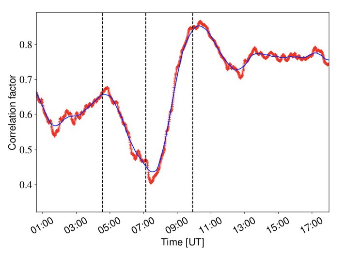
second time instant (07:07:30 UT), even if the values are over Fig. 8. Pearson coefficients for the vertical velocities in the region at the
centre of the FOV. The size of the window was 9000 × 6500 .
the zero line, it is possible to argue that both combinations fit
equally well. Then, after the third time instant (09:54:45 Ut), the
evolution shows that the best fitting is given by the combina- the plasma flows and the magnetic field element motions are well
tion of two Rayleigh distributions. On the other hand, Fig. 7d coupled. However, during the first magnetic emergence, the mo-
shows that in general for the continuum horizontal proper mo- tions become partly decoupled. This can be due to the idea that
tions, the distributions will be well fitted by the combination of in the first moment the newly emerging magnetic field is so pow-
two Rayleigh distributions, with the exception of some isolated erful and strong that it can weaken the coupling conditions for
short time instants that appear to coincide with the previously a moment, expand faster than the local surrounding plasma, and
outlined three special points of time we already discussed in Fig. only slightly later start also to push away the plasma. From about
6. On this occasions it appears that the best fitting is given using 3:00 UT to 4:00 UT the coupling between the continuum proper
the combination of one Rayleigh and one Gaussian distribution. motions and magnetic element motions are gradually restored,
just to be broken again and even more strongly by the second
emergence just after the first time instant mentioned above. This
4. Discussion time the coupling gets even more weakened indicating a stronger
In this work we have analysed time series of images display- emergence and stronger magnetic fields. Subsequently, after the
ing the formation of a solar active region in both continuum second time instant, this leads in the aftermath to a stronger
maps and LOS magnetograms. Results expose the presence of coupling of the continuum and magnetic field element motions
large-scale granular cells prior to the formation of the active re- most likely due to the governance of the magnetic field over the
gion. The horizontal proper motions show strong outflows (di- plasma owing to the strong emergence. After the third time in-
vergences) at the same places where strong upflows can be iden- stant, the flows become more stable and reach a high plateau of
tified. Although the calculated vertical velocities show upflows coupling with a correlation coefficient of up to 0.75. Thus we
in different sectors within the FOV, these emergences do not ex- would conclude that, at least during the emergence of the sec-
hibit strong and remarkable horizontal velocities. Besides, such ond magnetic bubble, the magnetic field was strong enough to
upflows are generally only related to the appearance and motion govern the plasma flows, while in other cases normal convection
of weak magnetic fields (< 10 Gauss). This is in strong con- might advect smaller magnetic elements.
trast to the horizontal velocities detected roughly in the centre Moreover, we can see in Fig. 8 that the maximum of correla-
of the FOV. Here it seems as if the strong upflows are also asso- tion happens co-temporarily with the large parameter deviations
ciated to the formation of AR 11190. Generally we would like as shown in Fig. 6a, identifiable in velocity distributions calcu-
to state that the behaviour of the continuum proper motions and lated for the magnetic field elements indicating again that the
the magnetic field element motions are strongly linked. This be- flow field is changing at these moments due to the emergence of
comes also very clear in the third row in Fig. 2, where both the new magnetic flux via the magnetic bubbles.
vertical velocities obtained from the horizontal velocities (back- As we have seen and outlined in the results section, the ve-
ground map) and the contours resulting from the positive ver- locity distributions, obtained from the flow maps, are well rep-
tical velocities obtained from the LOS magnetic field data are resented by the combination of two separate components. The
depicted together and display a strong correlation. This can be proposed two different combinations as given by Eqs. 4 and 5
clearly seen by applying a Pearson correlation analysis between feature both a Rayleigh distribution, which we would think of as
the vertical velocities from continuum maps and from the LOS fitting the undisturbed background flows, that is, the regions of
magnetic field. the FOV not affected by the flux emergence event, plus a second
Figure 8 shows exactly such calculated correlation and its component, which is variable in position and relative strength as
temporal evolution. The vertical dashed lines represent the same it applies for the occupied and effected area of the flux emer-
instants as mentioned in the Fig. 6. All of them are close to points gence process.
where the Pearson coefficient evolution changes its slope. In Fig. The open question to settle is, which one of the proposed compo-
8 we can see how the correlation starts at a value of around 0.65 nents generally fits better? The Gaussian or the Rayleigh distri-
indicating a good correlation before dropping at 2:00 UT to a lo- bution? We believe that it might not be clear as there could be a
cal minimum. This means that in the beginning of the time series kind of phase transition between both distributions. A Rayleigh
Article number, page 10 of 15J. I. Campos Rozo et al.: Plasma and magnetic field dynamics during the formation of AR 11190
distribution is formed for the magnitude of the velocity when 5. Conclusion
both vector components x and y are Gaussian distributed (in the
ideal case) with zero mean velocity and equal standard devia- In this paper we looked into the details of the evolving flow
tion, for example by a random walk process. Thus this kind of patterns in velocity maps during the formation of active region
a distribution is also a good candidate for the background flow 11190. The used data were obtained from the SDO/HMI instru-
and it might be a good candidate during weak emergences in ment as continuum maps and magnetograms to investigate both
which the additional flow component still follows more or less the continuum proper motions as well as the magnetic field ele-
a random walk but presumably with higher amplitudes. How- ment motions during two emergence events of positive flux lead-
ever, in the case of a strong flux emergence it is highly likely ing in consequence to the formation of the active region. Gener-
that all velocities in a larger and affected FOV area get directed ally we found a high congruence between the plasma flows and
away from the centre. Therefore, while the velocity amplitudes the motions of the magnetic elements. This congruence is weak-
might still be stronger and weaker, in some way the distribution ened and distorted during the emergence of new magnetic flux.
becomes one dimensional (only radially orientated away from Moreover, the speeds in the FOV can be fitted in general very
the centre of emergence) and hence the component representing accurately with a Rayleigh distribution. Nevertheless, during the
the affected flux emergence pixels follows to a greater extent a flux emergence events the Rayleigh distributions get distorted
Gaussian distribution instead of the Rayleigh one. A clearer in- and at least a secondary flow field component should be added.
sight could be gained by investigating in the future the formation It is plausible that this component can be either a secondary
of several active regions and looking then, with an even higher Rayleigh distribution with a larger width (higher velocities) dur-
focus, on the velocity distributions to study these last details, as ing the emergence or a Gaussian component. The stronger the
well as if and how, the secondary component changes. emergence, the more likely it is that the secondary component
follows a Gaussian distribution, which can be related to the idea
that strong emergences lead to radial outflows and, in that sense,
to a one-dimensional flow distribution (only a vr component ex-
ists, while normally the flow velocities are made up of a v x and
After the detailed discussion of the results above, we wish to a vy component). In order to support the statement about the ne-
contextualize our work within the larger field of solar physics. cessity of a two-component distribution, where the second com-
The evolution of active regions is an ongoing research field, es- ponent is formed due to the strong changes in the flow pattern
pecially in regards to the build up of magnetic energy for solar occurring during the formation of AR 11190, we analysed the
eruptions, so-called flares (see e.g. Kilcik et al. 2018; Ye et al. evolution of a quiet Sun region during the same day. We found
2018). This is generally done by having a detailed look into the that for a quiet Sun flow-field distribution it is sufficient to use
magnetic field evolution as well as its configuration over time a single Rayleigh distribution to fit the speeds distribution (see
(e.g. Dacie et al. 2016). Such investigations are often directly Fig. A.2). It is also possible to observe the temporal evolution of
performed by analysis of magnetograms but increasingly com- the fitting parameters over 4 hours (see Fig. A.3), and conclude
monly also by magnetic field extrapolations (e.g. Thalmann & that they do not show strong enhancements compared to their
Wiegelmann 2008). Another possibility for such analysis comes general behaviour.
via simulations and modelling (Cheung & DeRosa 2012). It is
very clear that for a successful modelling of the process of en- Acknowledgements. This research received support by the Austrian Science
Fund (FWF) P27800. Jose Iván Campos Rozo and Santiago Vargas Domínguez
ergy build up, detailed knowledge about the velocity fields trans- acknowledge funding from Universidad Nacional de Colombia research project
porting the magnetic field above the solar surface, as well as code 36127: Magnetic field in the solar atmosphere. Additional funding was
shredding and twisting the field lines, is of great importance. possible through an Odysseus grant of the Fund for Scientific Research-Flanders
The detailed measurement of flow fields, and derivation of the (FWO Vlaanderen), the IAP P7/08 CHARM (Belspo), and GOA-2015-014 (KU
Leuven). This work has also received funding from the European Research
velocity distributions, are not only important for the evolution Council (ERC) under the European Union’s Horizon 2020 research and inno-
of the active regions themselves, but indeed also necessary for vation programme (grant agreement No 724326). Jose Iván Campos Rozo is
large-scale flux transport models such as the advective flux trans- grateful to the National University, the Research Direction, and the National As-
port (AFT) model (see e.g. Ugarte-Urra et al. 2015). Thus a tronomical Observatory of Colombia for providing him with a travel grant under
better knowledge of the velocity fields will also help in the un- the project for new professors and researchers to spend a part of his thesis time at
KU Leuven enabling him to collaborate with Prof. T. Van Doorsselaere for this
derstanding of the global dynamo acting on the Sun. Such flux study. He also wishes to acknowledge the whole KU-Leuven University for the
transport models describe in a simplified way how the magnetic space and the academic support provided during his stay in Leuven. HMI/SDO
field emerges (e.g. in active regions), is shredded, and then trans- data are courtesy of NASA/SDO and the AIA, EVE, and HMI science teams,
ported via the velocity fields, including the meridional circula- and they were obtained from the Joint Science Operation Center (JSOC). Part of
this research has been created by using SunPy libraries, an open-source and free
tion and differential rotation, to the poles, where the fields finally community-developed solar data analysis package written in Python. We wish to
get submerged. Thus a better parametrization of the velocity express our gratitude to the editor of A&A, and the anonymous referee for his
fields as done for example in this study will be of importance for or her suggestions and comments about the present work, which improved the
such modelling efforts. A final interesting field for which this re- study considerably.
search might yield a new approach is the field of flux emergence
studies. Authors like Golovko & Salakhutdinova (2015) have
pointed out that flux emergence can be detected in image data References
by algorithms using sophisticated multi-fractal spectral analysis
and segmentation. On the other hand, we have shown now that Asensio Ramos, A., Requerey, I. S., & Vitas, N. 2017, A&A, 604, A11
Bushby, P. J. & Favier, B. 2014, A&A, 562, A72
not only the structures within the FOV are changed (classically Campos Rozo, J. I. & Vargas Dominguez, S. 2014, Central European Astrophys-
the granulation pattern gets elongated, which can be used within ical Bulletin, 38, 67
segmentation algorithms) but that the flow field changes remark- Cheung, M. C. M. & DeRosa, M. L. 2012, ApJ, 757, 147
Dacie, S., Démoulin, P., van Driel-Gesztelyi, L., et al. 2016, A&A, 596, A69
ably leading to changed velocity distributions. Thus by investi- de la Cruz Rodríguez, J., Hansteen, V., Bellot-Rubio, L., & Ortiz, A. 2015, ApJ,
gating the flow field statistics, one can also detect and character- 810, 145
ize flux emergence events. Domínguez Cerdeña, I. 2003, A&A, 412, L65
Article number, page 11 of 15A&A proofs: manuscript no. ms Golovko, A. A. & Salakhutdinova, I. I. 2015, Astronomy Reports, 59, 776 Guglielmino, S. L., Bellot Rubio, L. R., Zuccarello, F., et al. 2010, ApJ, 724, 1083 Hansen, C. J., Kawaler, S. D., & Trimble, V. 2004, Stellar Interiors, 2nd edn. (New York: Springer-Verlag), 241 Hill, F., Gough, D., & Toomre, J. 1984, Mem. Soc. Astron. Italiana, 55, 153 Hoeksema, J. T., Liu, Y., Hayashi, K., et al. 2014, Sol. Phys., 289, 3483 Hoffman, D., Karst, O. J., & Hoblit, F. M. 1975, Journal of Ship Research, 19, 172 Hurlburt, N. E., Schrijver, C. J., Shine, R. A., & Title, A. M. 1995, in ESA Special Publication, Vol. 376, Helioseismology, 239 Ishikawa, R. & Tsuneta, S. 2011, ApJ, 735, 74 Kilcik, A., Yurchyshyn, V., Sahin, S., et al. 2018, MNRAS, 477, 293 Lisle, J. & Toomre, J. 2004, in ESA Special Publication, Vol. 559, SOHO 14 Helio- and Asteroseismology: Towards a Golden Future, ed. D. Danesy, 556 Louis, R. E., Ravindra, B., Georgoulis, M. K., & Küker, M. 2015, Sol. Phys., 290, 1135 Márquez, I., Sánchez Almeida, J., & Bonet, J. A. 2006, ApJ, 638, 553 Massaguer, J. M. & Zahn, J.-P. 1980, A&A, 87, 315 Molowny-Horas, R. 1994, Sol. Phys., 154, 29 Musman, S. 1972, Sol. Phys., 26, 290 Namba, O. & van Rijsbergen, R. 1977, in Lecture Notes in Physics, Berlin Springer Verlag, Vol. 71, Problems of Stellar Convection, ed. E. A. Spiegel & J.-P. Zahn, 119–125 November, L. J. 1989, ApJ, 344, 494 November, L. J. & Simon, G. W. 1988, ApJ, 333, 427 November, L. J., Simon, G. W., Tarbell, T. D., & Title, A. M. 1986, in BAAS, Vol. 18, Bulletin of the American Astronomical Society, 665 November, L. J., Simon, G. W., Tarbell, T. D., Title, A. M., & Ferguson, S. H. 1987, in NASA Conference Publication, Vol. 2483, NASA Conference Pub- lication, ed. G. Athay & D. S. Spicer November, L. J., Toomre, J., Gebbie, K. B., & Simon, G. W. 1981, ApJ, 245, L123 Ortiz, A., Bellot Rubio, L. R., Hansteen, V. H., de la Cruz Rodríguez, J., & Rouppe van der Voort, L. 2014, ApJ, 781, 126 Palacios, J., Blanco Rodríguez, J., Vargas Domínguez, S., et al. 2012, A&A, 537, A21 Pesnell, W. D., Thompson, B. J., & Chamberlin, P. C. 2012, Sol. Phys., 275, 3 Potts, H. E., Barrett, R. K., & Diver, D. A. 2003, Sol. Phys., 217, 69 Rast, M. P. 2003, ApJ, 597, 1200 Rezaei, R., Bello González, N., & Schlichenmaier, R. 2012, A&A, 537, A19 Rieutord, M. & Rincon, F. 2010, Living Reviews in Solar Physics, 7, 2 Rösch, J. 1961, Il Nuovo Cimento, 22, 313 Roudier, T., Lignières, F., Rieutord, M., Brandt, P. N., & Malherbe, J. M. 2003, A&A, 409, 299 Roudier, T., Rieutord, M., Malherbe, J. M., & Vigneau, J. 1999, A&A, 349, 301 Schuck, P. W. 2006, ApJ, 646, 1358 Simon, G. W., Title, A. M., Topka, K. P., et al. 1988, ApJ, 327, 964 Simon, G. W., Title, A. M., & Weiss, N. O. 1995, ApJ, 442, 886 SunPy Community, Mumford, S. J., Christe, S., et al. 2015, Computational Sci- ence and Discovery, 8, 014009 Thalmann, J. K. & Wiegelmann, T. 2008, A&A, 484, 495 Title, A. M., Tarbell, T. D., Acton, L., Duncan, D., & Simon, G. W. 1986, Ad- vances in Space Research, 6, 253 Title, A. M., Tarbell, T. D., Topka, K. P., et al. 1989, ApJ, 336, 475 Ugarte-Urra, I., Upton, L., Warren, H. P., & Hathaway, D. H. 2015, ApJ, 815, 90 Vargas Dominguez, S. 2009, PhD thesis, PhD Thesis, 2009 Vargas Domínguez, S., van Driel-Gesztelyi, L., & Bellot Rubio, L. R. 2012, Sol. Phys., 278, 99 Verma, M., Denker, C., Balthasar, H., et al. 2016, A&A, 596, A3 Verma, M., Steffen, M., & Denker, C. 2013, A&A, 555, A136 Welsch, B. T., Fisher, G. H., Abbett, W. P., & Regnier, S. 2004, ApJ, 610, 1148 Ye, Y., Korsos, M. B., & Erdelyi, R. 2018, ArXiv e-prints [arXiv:1801.00430] Yi, Z., Darvann, T., & Molowny-Horas, R. 1992, Software for Solar Image Pro- cessing - Proceedings from lest Mini Workshop, Tech. rep. Article number, page 12 of 15
J. I. Campos Rozo et al.: Plasma and magnetic field dynamics during the formation of AR 11190

Appendix A: Comparison with quiet Sun
To show the necessity of the combined speed distribution in ac-
tive regions, we wish to replicate the analysis for a quiet Sun
region within the period of our data set (from 16:00 UT to 20:00
UT on the same day).6 Figure A.1 shows on the left-hand side
the full disc Sun on the day of observations, with the two anal-
ysed regions of interest marked by rectangles. The continuum
maps and magnetograms of the two regions are shown in the
right panels. Clearly the magnetic field activity is very high in
the active region, while it is practically non-existent in the quiet
Sun (as expected). We applied the LCT algorithm on the chosen
quiet Sun region. The data comprise 320 images with the same
cadence as described before and a total time of 4 hours. The pa-
rameters for the LCT algorithm are the same as in the case for
the active region. The principal first outcome can be seen in Fig.
A.2. Here we show the histograms of the speeds at three dif-
ferent times, which are independent and not related to the AR
11190 analysis. It becomes clear that a single Rayleigh distribu-
tion fits very well the whole histogram and it is not necessary,
compared to the active region data, to fit the histogram with a
more complex two-component distribution.
    As this could be only a special case for three times, we also
replicated Fig. 6 for the quiet Sun as shown in Fig. A.3. The evo-
lution of the parameters shows no significant events (like strong
parameter deviations), except for a few small occasional changes
for the combination of Rayleigh distribution with a Gaussian
component. Thus, again we can see that within the quiet Sun
the expected result was realized, namely, the possibility to create
a good single Rayleigh component fit. This is fully understand-
able as this principal distribution will be formed due to random
x/y motions created from the turbulent convection.

6
   An analysis of a plage region would complement this study perfectly,
however, due to the considerable size of the current study and the nec-
essary analysis, we postpone such an analysis to a future investigation.

                                                                                                               Article number, page 13 of 15
You can also read