Quantifying impacts of the drought 2018 on European ecosystems in comparison to 2003 - arXiv
←
→
Page content transcription
If your browser does not render page correctly, please read the page content below
Quantifying impacts of the drought 2018 on European ecosystems in
                             comparison to 2003
Allan Buras1, Anja Rammig1, Christian S. Zang 1
1*
 Technical University of Munich, TUM School of Life Sciences Weihenstephan, Professorship for
Land Surface-Atmosphere Interactions, Hans-Carl-von-Carlowitz Platz 2, 85354 Freising, Germany.

*Correspondence:
Allan Buras

allan@buras.eu

Keywords: Remote sensing, Compound events, Drought legacy, Ecosystem productivity,
Climatic water balance, Atmospheric circulation patterns.

Abstract

In recent decades, an increasing persistence of atmospheric circulation patterns has been observed. In
the course of the associated long-lasting anticyclonic summer circulations, heat waves and drought
spells often coincide, leading to so-called hotter droughts. Previous hotter droughts caused a decrease
in agricultural yields and increase in tree mortality, and thus, had a remarkable effect on carbon budgets
and negative economic impacts. Consequently, a quantification of ecosystem responses to hotter
droughts and a better understanding of the underlying mechanisms is crucial. In this context, the
European hotter drought of the year 2018 may be considered as a key event. As a first step towards the
quantification of its causes and consequences, we here assess anomalies of atmospheric circulation
patterns, temperature loads, and climatic water balance as potential drivers of ecosystem responses as
quantified by remote sensing using the MODIS vegetation indices NDVI and EVI. To place the drought
of 2018 within a climatological context, we compare its climatic features and ecosystem response with
the extreme hot drought of 2003. Our results indicated 2018 to be characterized by a climatic dipole,
featuring extremely hot and dry weather conditions north of the Alps but comparably cool and moist
conditions across large parts of the Mediterranean. Analyzing ecosystem response of five dominant
land-cover classes, we found significant positive effects of April-July climatic water balance on
ecosystem productivity. Negative drought impacts appeared to affect a larger area and to be
significantly stronger in 2018 compared to 2003. Moreover, we found a significantly higher sensitivity
of pastures and arable land to climatic water balance compared to forests in both years. The stronger
coupling and higher sensitivity of ecosystem response in 2018 we explain by the prevailing climatic
dipole: while the generally water-limited ecosystems of the Mediterranean experienced above-average
climatic water balance the less drought-adapted ecosystems of Central and Northern Europe
experienced a record hot drought. In conclusion, this study quantifies the drought of 2018 as a yet
unprecedented event and provides valuable insights into the heterogeneous responses of European
ecosystems to hotter drought.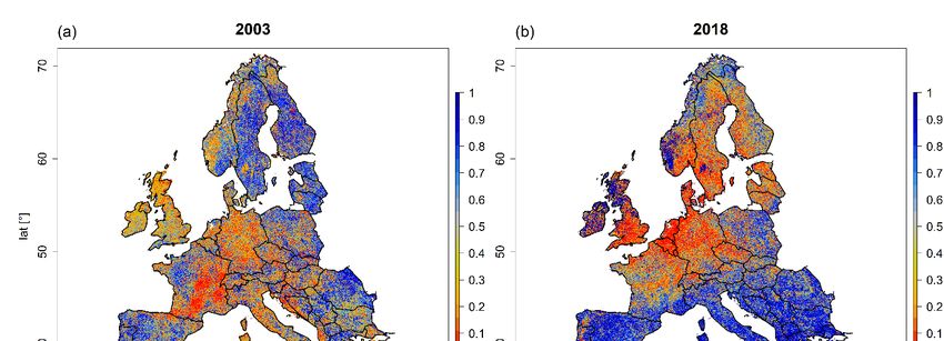
1     Introduction

More frequent and longer-lasting heat waves are expected to occur with global warming (IPCC, 2014).
If such heat waves coincide with low precipitation sums, so-called ‘global-change type droughts’ or
‘hotter droughts’ emerge (Allen et al., 2015; Breshears et al., 2005). In the course of hotter droughts,
positive feedback loops related to a non-linearly amplified soil-water depletion through
evapotranspiration (Seneviratne et al., 2010) further aggravate surface-temperature anomalies because
of reduced latent cooling (Fischer et al., 2007). To emphasize this interdependence of heat and drought
and improve projections of potential high-impact events, hotter droughts were recently classified as
compound events (Zscheischler et al., 2018). Accounting for the interdependence of climatic drivers
for drought, climate model projections generally indicate an increase in the likelihood of a hotter
drought during the 21st century (Zscheischler and Seneviratne, 2017). Given the associated climatic
properties, hotter droughts are more likely to occur under abnormally stable anticyclonic atmospheric
circulation patterns which were recently shown to be connected with a hemisphere-wide wavenumber
7 circulation pattern (Kornhuber et al., 2019). Abnormally stable anticyclonic atmospheric circulation
patterns and associated wavenumber 7 circulation patterns have expressed an increasing frequency
over the past decades (Horton et al., 2015; Kornhuber et al., 2019).

Hotter droughts feature a wide range of negative impacts on managed and natural ecosystems, e.g.
reduced productivity, which has been indicated by lower vegetation greenness using remote sensing
data (Allen et al., 2015; Choat et al., 2018; Ciais et al., 2005; Orth et al., 2016; Xu et al., 2011). As a
consequence, agricultural yields decline remarkably during hotter droughts while drought-induced tree
mortality increases, with both effects leading to significant economic losses (Allen et al., 2010; Buras
et al., 2018; Cailleret et al., 2017; Choat et al., 2018; Ciais et al., 2005; Matusick et al., 2018).
Moreover, since gross primary productivity (GPP) decreases during hotter droughts, the resulting lower
net carbon uptake may change ecosystems from carbon sinks into carbon sources (Ciais et al., 2005;
Xu et al., 2011). However, the response to drought may vary among different land-cover types,
particularly between grasslands and forests (Teuling et al., 2010; Wolf et al., 2013).

On the continental scale, the European heat wave of 2003 is to date considered as the most extreme
compound event in Europe with various impacts on human health (increased mortality particularly in
France), economy (decreased crop yield in agriculture and forestry), and ecosystems (reduced
productivity, forest die-back, and an increased frequency of forest fires; Fink et al., 2004; García-
Herrera et al., 2010). According to Ciais et al. (2005), GPP of European ecosystems was reduced by
30 percent in summer 2003 – a yet unprecedented reduction in Europe’s primary productivity which
resulted in an estimated net carbon release of 0.5 PG C yr-1. Given the wide-ranging impacts, potential
climate change feedback loops, and the increasing frequencies of circulation patterns initiating
compound events it is pivotal to better understand and thus more precisely predict the response of
managed and natural ecosystems to hotter droughts (Horton et al., 2015; Pfleiderer and Coumou, 2018;
Sippel et al., 2017; Zscheischler and Seneviratne, 2017).

In the context of an increased persistence of circulation patterns, the European drought of 2018 is of
particular interest. In April 2018, a high-pressure system established over Central Europe and persisted

                                                                                                        2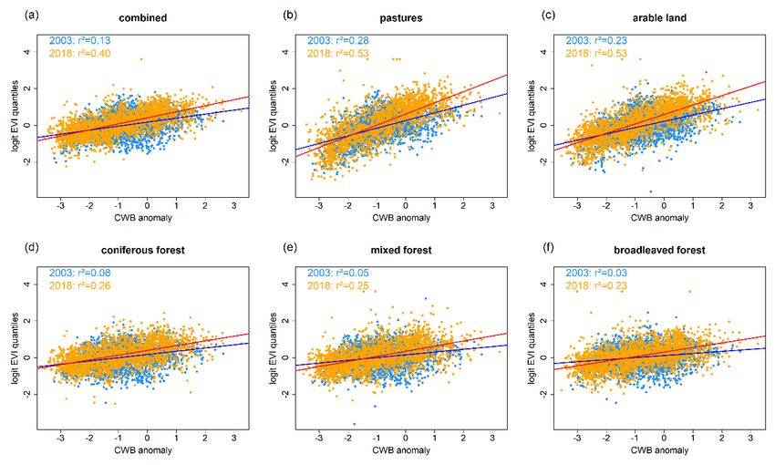
almost continuously until mid of October, thereby causing a long-lasting drought spell and record
temperatures in central and northern Europe. Despite preliminary reports in public news and the world-
wide-web (see list of public news references), the direct impacts resulting from the 2018 drought are
still unexplored. Consequently, we here quantify the impacts of the extreme drought of 2018 on
European ecosystems in comparison to the extreme drought in the year 2003. Thereby, we 1) provide
an estimate of European ecosystems immediate response to the drought 2018 in relation to 2003, 2)
identify hotspots of extreme drought and associated ecosystem response, and 3) aim at an improved
mechanistic understanding of the processes driving ecosystem responses to extreme drought events.

2   Material and Methods

2.1 Data sources and preparation

2.1.1 Climate data

To visualize the general circulation patterns in 2003 and 2018 we downloaded gridded reanalysis data
representing 500 hPa geopotential height from the NCEP/NCAR Reanalysis project provided by the
NOAA climate prediction center (Kalnay et al., 1996) available at the Earth System Research
Laboratory (ESRL, https://www.esrl.noaa.gov/). The downloaded data cover the period 1981-2018 at
a daily temporal resolution and a spatial resolution of 2.5°. As a representation of high-pressure
persistence, we computed the mean geopotential height for each grid cell and year for the period from
1st of April until 31 st of July.

From ESRL, we furthermore downloaded reanalyzed (NCEP/NCAR), daily gridded mean minimum
and maximum temperature (T min, Tmax) and precipitation (P) sums at 0.5° spatial resolution covering
the period 1981-2018 (Kalnay et al., 1996). These variables were used to compute potential
evapotranspiration (PET, as defined by Hargreaves, 1994) and the climatic water balance (CWB = P-
PET, Thornthwaite, 1948). As for geopotential height, we for each grid cell and year integrated T max
and CWB for the period from 1 st of April until 31 st of July as measures of heat load and water balance.

Processed climate data were spatially truncated to match the region considered for the MODIS satellite
images (see next section) resulting in 2312 climate grid cells representing an area of roughly 5.9 million
km² and covering 38 years. To allow for combination with MODIS data throughout the analyses,
processed climate data were re-projected to MODIS native projection using zonal means while
retaining a spatial resolution of 0.5°.

To locally quantify climatic conditions, we furthermore extracted monthly temperature means and
precipitation sums for six climate stations from the European Climate Assessment and Data project
(Tank et al., 2002) available at the corresponding project webpage (www.ecad.eu). We chose Oslo and
Stockholm, Amsterdam and Berlin, as well as Madrid and Sevilla to represent weather conditions in
Northern, Central, and Southern Europe, respectively. Monthly temperature means and precipitation
sums of 2003 and 2018 were visually compared to average values representative of the climate normal
period 1961-1990.

                                                                                                       3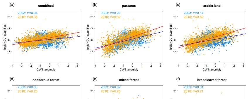
2.1.2   MODIS vegetation indices

Using the Application for Extracting and Exploring Analysis Ready Samples (AppEEARS;
https://lpdaacsvc.cr.usgs.gov/appeears) we downloaded two MODIS vegetation indices (VI, i.e. the
Normalized Difference Vegetation Index NDVI and the Enhanced Vegetation Index EVI) and the
corresponding pixel reliability layers at 231 m spatial resolution and 16 day temporal resolution in their
native projection. The downloaded data cover the area between 10° E and 30° W longitude, 36.5° N
and 71.5° N latitude that is represented by the CORINE land cover information of 2012 (see section
2.1.3) and span the period from February 2000 until end of 2018.

Based on the pixel reliability information, we only retained records with good or marginal quality for
subsequent analyses. Consequently, for most of the grid cells the VI time series contained missing
values due to temporary clouds or snow cover. If the number of missing values was larger than the
number of VI records, we considered the representing records as insufficient for our analyses and
consequently removed the corresponding pixel from the analysis. However, since high-elevation as
well as high-latitude pixels had many missing values in winter and spring because of clouds and snow
cover and we only were interested in VI during peak season, we only considered the period from
beginning of March (DOY 64) to end of October (DOY 304) for the definition of valid pixels.
Following these selection criteria, we retained 95,523,236 pixels for the final analyses, representative
of an area of 5,970,202 km².

Prior to the analyses, VI time series of the retained pixels were further processed. We linearly
interpolated the missing values of the corresponding VI time series for each pixel using the previous
and succeeding records (Misra et al., 2016, 2018). Next, VI time series were detrended by computing
a mean VI time series over all grid cells (Fig. S1) and subtracting this total-scene time series from all
individual pixel time series. This consistent detrending was necessary to compensate for the observed
positive trend in vegetation indices (Bastos et al., 2017) which also was apparent in the downloaded
data (Fig. S1). A comparison between non-detrended and detrended data revealed similar spatial
patterns with respect to between-pixel variability, however with amplified differences between 2003
and 2018 in the raw, non-detrended data. That is, for the raw data, the observed trend caused lower
peak-season VI values in 2003 compared to 2018, thereby introducing an offset between these two
drought events. Concluding, the detrending was able to efficiently handle the positive VI-trend over
the MODIS-era, while spatial patterns were generally retained.

Subsequently, we removed negative outlier values from each VI time series by computing standardized
residuals to a Gaussian-filtered (filter size of 80 days, i.e. 5 MODIS time steps), smoothed time-series.
Residuals exceeding two negative standard deviations were replaced by the equivalent value of the
smoothed time series (see also Misra et al., 2018, 2016). Finally, we smoothed the interpolated, outlier-
corrected time series by reapplying the Gaussian filter. This procedure was necessary to efficiently
handle the remaining high-frequency variability in the seasonal VI-cycle (Misra et al., 2016, 2018).

Both NDVI and EVI are considered as proxy for photosynthetic carbon fixation, and thus allow for
assessing possible changes in productivity in dependence of environmental conditions (Huete et al.,
2006; Myneni et al., 1995; Xu et al., 2011). For reasons of simplicity, we focus on results derived from
                                                                                                       4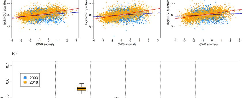
NDVI which are generally confirmed by results derived from EVI. To allow for a direct comparison
of NDVI and EVI results, the latter are depicted in the supplementary.

2.1.3   CORINE land cover information

To get an impression on the drought-impact on key European ecosystem components, analyses were
stratified using the Coordinated Information on the European Environment land cover map (CORINE,
https://land.copernicus.eu/pan-european/corine-land-cover/clc-2012) at 250 m spatial resolution. The
land cover map was re-projected (as were the gridded climate data) to MODIS native projection using
the nearest neighbor method, thereby retaining the original land-cover classes. Given their dominance
in Europe and their importance for land-use, we constrained this stratification to pastures, arable land,
as well as coniferous, mixed, and broadleaved forests.

2.2 Statistical analyses

To quantify weather conditions for the years 2003 and 2018 in relation to average conditions,
standardized anomalies of 500 hPa geopotential height, heat load and CWB were calculated. Before
doing so, we tested the underlying assumption of normal distribution by computing Shapiro test for
each grid cell and climate parameter respectively (Fig. S2). The number of significant tests (p < 0.001)
indicating non-normal distribution was in the order of expected false positives (0.0-0.3 percent vs. 0.1
percent type I error probability). Thus, we considered the assumption of normality to be generally
fulfilled. To derive anomalies, we first computed the mean and standard deviation for all variables for
the full period (1981-2018). Subsequently, we for 2003 and 2018 determined the difference of the
respective metric to its corresponding mean in units of standard deviations which in the following are
called standardized anomalies (this procedure is also known as z-transformation). Thus, for integrated
geopotential height, heat load, and CWB we obtained each one standardized anomaly per grid cell for
2003 and 2018. The resulting standardized anomalies were mapped and statistically evaluated using
histograms. Histograms were used to depict the absolute area of differently affected regions in 2003
and 2018 which were compared among each other as well as to a normal distribution. This was done
in order to visualize the severity of these two drought events in comparison to each other as well as in
comparison to normal conditions.

To quantify the response of European ecosystems to the two drought events, we focused on end-of-
July (DOY 209) VI values. The selection of this particular date represents a compromise between
proximity to peak-season (end of June, before maximum temperatures had been reached) and the
occurrence of heat-waves (end of July to mid of August). Since VI features a bounded distribution
(values between -1 and +1), we could not apply a standardization approach as for the climate variables.
Therefore, we for each VI time series computed its end-of-July quantiles over the 19 years similar to
Orth et al. (2016). The corresponding quantiles were mapped for 2003 and 2018. Areas representing
the 19 different quantiles were extracted and compared between 2003 and 2018 in a histogram.

Since we were aiming at a better understanding of particular ecosystems’ response to drought severity,
we subsequently pooled VI quantiles according to three classes of CWB anomalies (abnormal water
deficit: CWB < -2, average water supply: -2 < CWB < 2, abnormal water surplus: CWB >2) and five

                                                                                                      5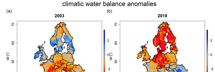
CORINE land-cover classes (arable land, pastures, coniferous forest, mixed forest, broadleaved forest).
For the resulting 15 combinations, we again compared the areas representing the 19 different quantiles
between 2003 and 2018 as done for the total scene. Since the areas of CWB-land cover combinations
differed between 2003 and 2018, we moreover computed histograms expressing proportional areas for
2003 and 2018.

Finally, we aimed at developing empirical relationships between CWB anomalies and VI quantiles for
the five CORINE land-cover classes mentioned before. For this, we logit transformed VI-quantiles
(quantiles ranging from 0 to 1) to obtain an unbounded distribution and subsequently extracted the
corresponding mean of transformed VI-quantiles for each CWB grid-cell (thus n = 2312). To assess
the effect of different land cover classes, we extracted both the mean EVI-quantiles representing all
five land cover classes as well as for each land cover class separately. For the corresponding 2312
CWB-pixels we computed linear regressions between the transformed EVI-quantiles as the dependent
variable and CWB anomalies as independent variable separately for 2003 and 2018 and for the six
different land cover types (i.e. five separate classes as well as their combination).

For linear regression evaluation, we report adjusted r² and display scatterplots of VI quantiles vs. CWB
along with the corresponding regression line. Moreover, regression slopes were compared statistically
for each land cover type between 2003 and 2018. For this, each slope estimate was bootstrapped using
random subsampling over 1000 iterations and the overlap of 95 % (99 %) confidence intervals was
evaluated. That is, in case the confidence intervals of a respective comparison did not overlap, we
considered the difference between slopes as (highly) significant. In a similar manner, we compared
model slopes among ecosystems (i.e. pastures, arable land, as well as coniferous, mixed, and deciduous
forest) separately for 2003 and 2018. Model slopes were grouped according to their overlap of 95 %
confidence intervals. Finally, we also computed a global model by applying a linear mixed effects
model (lme) to model EVI quantiles using climatic water balance as fixed effect and incorporating
crossed random slopes of land cover and year. All analyses were performed in ‘R’ (R core team, 2019)
extended for the packages, ‘nlme’ (Pinheiro et al., 2018), ‘raster’ (Robert J. Hijmans, 2017), and ‘SPEI’
(Beguería and Vicente-Serrano, 2013).

3 Results

All considered climate parameters indicated abnormal weather conditions for 2018 (Figs. 1-3). First of
all, the integrated 500 hPa geopotential height, an indicator of the persistence of the atmospheric
circulation, expressed anomalies in the order of two positive standard deviations for large parts of
Central and Northern Europe, mainly covering the Baltic Sea region (Fig. 1 b). In comparison, 2018
differed from 2003 by featuring a dipole of 500 hPa geopotential height anomalies. While in 2003 most
of Europe featured strong positive anomalies, the Mediterranean was characterized by low geopotential
height anomalies in 2018 (Fig. 1 a vs. Fig. 1 b). Consequently, the observed dipole of 2018 expressed
a bimodal distribution of anomalies whereas 2003 featured a skewed distribution towards positive
anomalies (Fig. 1c). The bimodal distribution of 2018 compared to 2003 is also reflected in a 0.55
times as large area featuring positive anomalies, i.e. 3.1 million km² in 2018 vs. 5.7 million km² in
2003, but a 3.7 times higher area with negative anomalies, 3.5 million vs. 0.9 million km² (Fig. 1c).

                                                                                                      6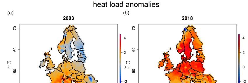
Fig. 1: Maps depicting standardized anomalies of April-July 500 hPa geopotential height for 2003 and
2018 (a, b) as well as corresponding area histograms (in units of 1000 km²) for 2003 (blue), 2018
(orange), compared to a normal distribution (black) (c). Blue colors in (a) and (b) indicate geopotential
height lower than average, whereas red colors indicate above average geopotential height in
comparison to the 1981-2018 mean.

This picture was underlined by heat-load anomalies, which revealed up to four positive standard
deviations over large parts of Central and Northern Europe in 2018 (Fig. 2 b). In contrast, the
Mediterranean featured average conditions (i.e. slightly warmer or cooler) as well as strong negative
anomalies on the Iberian Peninsula. Although the total area with positive heat-load anomalies was more
or less similar in 2003 and 2018 (Fig. 2b vs. 2a), anomalies above two positive standard deviations

                                                                                                      7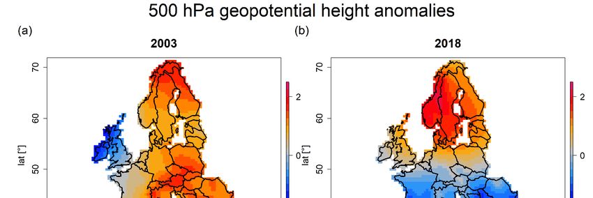
covered a 7.1 times larger area in 2018, i.e. 3.3 million km² vs. 0.5 million km² in 2003 (Fig. 2c). Most
contrasting differences between 2003 and 2018 were observed in Southern Italy (hot in 2003, cool in
2018) as well as Scandinavia and the Baltic Sea region (cool in 2003, hot in 2018). Selected climate
station data generally supported the impression of higher (lower) heat loads in 2018 compared to 2003
in Northern (Southern) Europe (Fig. S3a).

Fig. 2: Maps depicting standardized anomalies of April-July heat load for 2003 and 2018 (a, b) as well
as corresponding area histograms (in units of 1000 km²) for 2003 (blue), 2018 (orange), compared to
a normal distribution (black) (c). Blue colors in (a) and (b) indicate relatively cool conditions, whereas
red colors indicate warmer conditions in comparison to the 1981-2018 mean.

                                                                                                       8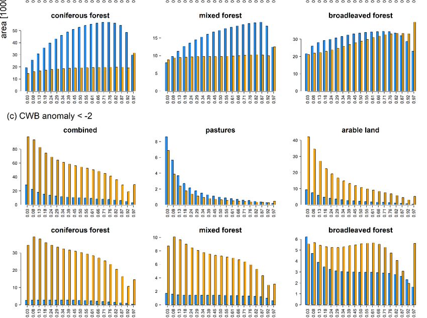
CWB for 2018 revealed patterns largely consistent with heat load (Fig. 3b). Again, Central and
Northern Europe featured extreme negative (thus dry) deviations, while the Mediterranean generally
expressed positive (thus moist) deviations. In comparison (Fig. 3b vs. 3a), the area with negative (i.e.
dry) CWB anomalies was relatively similar in both years, i.e. 4.2 million km² in 2018 vs. 4.6 million
km² in 2003 (Fig. 3c). However, when considering only CWB anomalies below two negative standard
deviations (i.e. extreme drought), in 2018 an area 5.3 times larger than in 2003 was affected, i.e. 1.7
million km² in 2018 in vs. 0.3 million km² in 2003 (Fig. 3c). Selected climate station data generally
supported the impression of higher (lower) water deficit in 2018 compared to 2003 in Northern
(Southern) Europe (Fig. S3b).

                                                                                                     9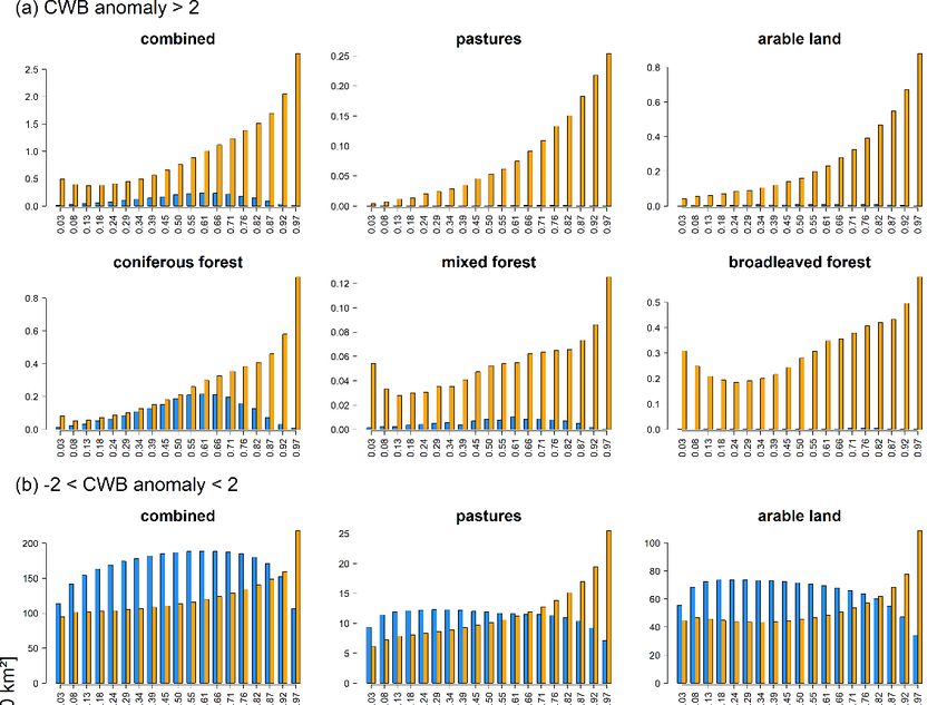
Fig. 3: Maps depicting standardized anomalies of April-July climatic water balance for 2003 and 2018
(a, b) as well as corresponding area histograms (in units of 1000 km²) for 2003 (blue), 2018 (orange),
compared to a normal distribution (black) (c). Blue colors in (a) and (b) indicate relatively moist
conditions, whereas red colors indicate dryer conditions in comparison to the 1981-2018 mean.
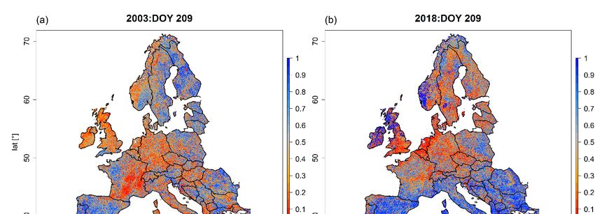
End of July vegetation response indicated clear differences between 2003 and 2018. We found low
NDVI quantiles in large parts of Central Europe, Southern Scandinavia, and the Baltic Sea region and
high quantiles in the Mediterranean in 2018 (Fig. 4b). In comparison, 2003 featured low NDVI
quantiles in Western, Central, and Southeast Europe and heterogeneous patterns in Northern Europe
(Fig. 4a). The most prominent difference between 2018 and 2003 was the 3.8 times larger area featuring
the highest quantile, i.e. 796,814 km² in 2018 vs. 210,876 km² in 2003 (Fig. 4c). At the same time, a
1.6 times larger area featured the lowest quantile in 2018, i.e. 481,513 km² vs. 294,377 km² in 2003
(Fig. 4c). According to NDVI quantiles, hotspots of drought-response in 2018 were located in the
Southern United Kingdom, Central France, Belgium, Luxemburg, the Netherlands, Northern
Switzerland, Germany, Denmark, Sweden, Southern Norway, Czech Republic, Lithuania, Latvia,
Estonia, and Finnland.
In regions with water deficit (CWB < - 2; Figs. 5c and S4c) we found a higher frequency of low NDVI
quantiles compared to upper quantiles. Similarly, regions with water surplus (CWB > 2; Figs. 5a and
S4a) featured higher frequencies for upper quantiles compared to lower quantiles which however was
more pronounced in 2018 compared to 2003. Interestingly, normal conditions (Figs. 5b and S4b)
revealed a tendency towards higher frequencies for upper quantiles in 2018 for all land-cover classes
whereas 2003 featured an inconsistent picture for the different land-cover classes. The most prominent
difference was related to absolutely larger areas being affected by water deficit and surplus in 2018
compared to 2003. If considering relative frequencies, histograms of 2018 and 2003 became more
similar (Fig. S4).
The impression of CWB affecting NDVI quantiles was underlined by the linear regressions between
the logit-transformed NDVI quantiles and the CWB-anomaly in 2003 and 2018, respectively (Fig. 6a-
f). That is, for all land-cover classes a significant and positive effect of climatic water balance on NDVI
quantiles was observed, particularly in 2018. Interestingly, explained variance (r²) and bootstrapped
model slopes were consistently higher in 2018 compared to 2003 (Fig. 6 g). In addition, r² and model
slopes were in both years highest for pastures, followed by arable land, and the three forest types which
did not differ among each other (lower case letters in Fig. 6g). The linear mixed effects model over all
land-cover classes and the two years confirmed the significant fixed effect of climatic water balance
on logit-transformed NDVI quantiles (marginal r² = 0.19). Incorporation of random slopes related to
land cover and year resulted in a remarkable increase in explained variance (conditional r² = 0.29) of
33 percent, confirming the varying effect of the two drought events as well as the differing impact on
different land-cover classes. All presented results based on NDVI are generally confirmed by
complementary analyses using EVI (supplementary Figs. S5-S8).
10Fig. 4: MODIS NDVI quantiles representing peak-season conditions at the end of July (DOY 209) in
2003 (a) and 2018 (b) as well as the corresponding area histograms (in units of 1000 km²) representing
the nineteen NDVI quantiles (c). Blue colors in (a) and (b) indicate upper quantiles (thus a higher than
average vegetation greenness), while orange to red colors indicate lower anomalies (i.e. lower than
average vegetation greenness). Blue bars in (c) refer to 2003 and orange bars to 2018. Similar results
for MODIS EVI are shown in supplementary Fig. S5.
11Fig. 5: Histograms depicting the absolute areas (in units of 1000 km²) representing the nineteen NDVI
quantiles pooled according to CORINE land-cover classes for regions that featured (a) water surplus
(CWB-anomaly > 2), (b) average conditions (- 2 < CWB-anomaly < 2), and (c) water deficit (CWB-
anomaly < -2). Blue bars refer to 2003, orange bars to 2018. Similar results for MODIS EVI are shown
in supplementary Fig. S6.
12Fig. 6: (a-f) Scatterplots depicting the relationship between average logit-transformed NDVI-quantiles
and mean CWB of the 100 CWB percentiles in 2003 (blue) and 2018 (orange) for pastures (b), arable
land (c), coniferous forests (d), mixed forest (e), broadleaved forest (f) and a combination of those (a).
Blue lines depict the regression line for 2003, red lines for 2018. (g) Bootstrapped regression slope
estimates for the five different land-cover classes as well as their combination. Minor case letters refer
to group assignment of land-cover classes according to the overlap of 99.9 % confidence intervals of
bootstrapped slopes in 2003 (blue) and 2018 (orange). Significance stars (***) indicate no overlap
between 99.9 % confidence intervals of 2003 and 2018 for the respective land-cover class. PS =
pastures, AL = arable land, CF = coniferous forest, MF = mixed forest, BF = broadleaved forest.
Similar results for MODIS EVI are shown in supplementary Fig. S8.
134 Discussion
4.1 Climatic framework
Based on the parameters considered for the quantification of summer conditions, 2018 clearly
supersedes 2003 (Figs. 1-3). That is, the anomaly of integrated 500 hPa geopotential height indicated
more persistent anticyclonic circulation patterns for 2018 across Northern Europe, which likely
triggered the strong positive heat load anomalies and negative climatic water balances across Central
and Northern Europe in comparison to 2003. Altogether, the area featuring strong positive heat load
anomalies and strong negative climatic water balance anomalies was respectively 7.1 and 5.3 times
larger in 2018, compared to 2003. However, another specific feature of 2018 in comparison to 2003 is
the clear dipole of 500 hPa geopotential height, which resulted in lower heat loads and an above average
climatic water balance in the Mediterranean.
Anticyclonic blocking situations – as indicated by strong positive 500 hPa geopotential height
anomalies – have been reported an increasing frequency in course of the satellite era (Horton et al.,
2015) which likely relates to the increasing persistence of heatwaves observed over the past 60 years
(Pfleiderer and Coumou, 2018) and the increasing frequency of a hemisphere-wide wavenumber 7
circulation pattern (Kornhuber et al., 2019). The resulting heatwaves are additionally enhanced by
global warming and positive land surface – atmosphere feedback loops via soil moisture depletion and
subsequent lack of latent cooling (Fischer et al., 2007). Moreover, summer temperatures and
precipitation were reported to correlate negatively at mid latitudes which may amplify further
according to CMIP5 climate projections (Zscheischler and Seneviratne, 2017). This renders the
evaluation of ecosystem responses to compound events a key topic for climate change research
(Zscheischler et al., 2018). Consequently, the persistent climatic blocking situation which resulted in a
large spatial distribution of extreme temperature and water balance anomalies qualifies 2018 as a key
event for studying ecosystem-responses to anticipated hotter droughts in Europe.
4.2 Ecosystem impact
End of July MODIS NDVI anomalies generally supported the impression of a more extreme drought
in 2018. That is, the area featuring the lowest quantile in 2018 was roughly 190,000 km² larger
compared to 2003 (Fig. 4c). In accordance with the more northward location of the anticyclone,
hotspots of ecosystem impact were concentrated in Central and Northern Europe in 2018. At the same
time, large parts of the Mediterranean featured positive NDVI deviations in 2018 which resulted in a
3.6 times larger area represented by the highest NDVI quantile compared to 2003 (Fig. 4c).
In general, the spatial distribution of NDVI quantiles matches the observed climatic dipole of 2018
very well (see section 4.1). Moreover, the bimodal response of European ecosystems is well in line
with a preliminary report on European maize yield in 2018, with an observed strong increase (10%
more than average) for e.g. Romania and Hungary, a strong decrease (10% less than average) for e.g.,
Germany and Belgium, and the European level net effect estimated at a decrease in maize yield of
around 6% (see public references: European Commission).
14The bimodal behavior and larger extent of ecosystem impact in 2018 was also reflected in land-cover
specific area distributions of NDVI quantiles (Fig. 5a and 5c). That is, the area featuring lowest
(highest) quantiles in regions with water deficit (surplus) was much larger in 2018 compared to 2003.
Given the skewed distribution of quantiles in those regions, i.e. more lower quantiles in regions with
strong negative CWB anomalies and more upper quantiles in regions with strong positive CWB
anomalies, the response of these ecosystems appears to be governed by prevailing climate conditions.
This impression was underlined by linear regressions, which revealed a strong and significant positive
impact of CWB on NDVI quantiles in both years and for all land-cover types (Figs. 6a-f). It is
noteworthy, that 2018 was characterized by a higher explained variance and significantly more positive
model slopes in comparison to 2003 (Fig. 6g). These impressions from single linear models were
generally supported by the linear mixed effects model, which showed an increase of r² at about 33
percent when incorporating land-cover and year as random effects.
The stronger coupling between CWB and NDVI quantiles in 2018 may be related to the period used to
integrate CWB (April-July). To test this, we assessed the relationship of NDVI quantiles with CWB
integrated over various different periods (e.g. including previous winter in CWB or shortening the
period) which all revealed similar patterns, i.e. a stronger response to CWB in 2018 (not shown).
However, it seems possible that the stronger coupling of NDVI quantiles with CWB in 2018 is related
to the spatial distribution of drought and thus the ecosystems being affected. In 2003, the epicenter of
the drought was located in Central France and the Mediterranean, i.e. regions which host ecosystems
that are regularly experiencing summer drought and thus are likely better adapted to dry conditions. In
contrast, the circulation patterns of 2018 resulted in a drought-epicenter in Central Europe, Southern
Scandinavia, and around the Baltic Sea, i.e. regions with ecosystems which are less adapted to
extremely dry climatic conditions such as in 2018 and therefore likely react strongly. Various reports
from dried-out pastures and cornfields as well as deciduous trees shedding their leaves in July and
August likely explain the record-low NDVI values for corresponding Central European ecosystems
(see public news references). At the same time, the usually summer-dry Mediterranean experienced
water surplus, relaxing the general limitation of the associated ecosystems by plant water availability
and leading to a generally higher greenness of the vegetation. Considering forest ecosystems, this
interpretation is in in line with Klein (2014), who reported higher leaf gas exchange and thus
photosynthetic capacity under dry conditions in Mediterranean forests compared to temperate forests.
Nevertheless, our hypothesis explaining the stronger coupling of NDVI quantiles with CWB in 2018
needs further investigation, e.g. by studying the sensitivity and coupling of plant productivity with
climatic properties for the considered land-cover classes as for instance done by Anderegg et al. (2018).
A sub-classification of land-cover classes seems to be reasonable for such an analysis, in order to
account for possibly differing drought-sensitivities of ecosystems represented by one specific land-
cover class. For instance, Mediterranean coniferous forests are likely more adapted to drought
conditions than boreal coniferous forests in Scandinavia.
In addition to the differences between the two drought events, we also observed differing sensitivities
of NDVI quantiles to CWB among ecosystems, which were consistent over the two drought events.
We found the highest regression slope estimates for pastures followed by arable land, coniferous
15forests, mixed forests, and broadleaved forests (Fig. 6g). This likely reflects the higher climatic
buffering function of forests in comparison to arable land and pastures. In forests, the micro-climate is
generally less extreme, leading to lower ambient air temperatures and consequently a lower
evapotranspiration in comparison to open fields (Chen et al., 1993, 1999; Young and Mitchell, 1994).
Consequently, water resources are consumed more sustainably by forests. Moreover, if not growing on
water-logged soils trees typically feature higher rooting depths compared to grasses and crops and
therefore have access to deeper soil water reservoirs. Regarding the European drought of 2003, an
accelerated soil moisture depletion of grasslands in comparison to forests has been reported earlier
(Teuling et al., 2010). Also Wolf et al. (2013) found contrasting responses of grasslands vs. forests
regarding water and carbon fluxes during a drought event in 2011. They observed an immediate
negative drought-impact on the productivity of managed grasslands while mixed and coniferous forests
simply reduced transpiration and maintained GPP, thereby increasing their water-use efficiency and
decreasing soil-water consumption (Wolf et al., 2013).
Nevertheless, European forests were in parts heavily affected by the drought 2018, as indicated by the
depicted density distributions (Fig. 5c). For instance, 60,000 km² of drought affected coniferous forests
featured the lowest quantile in 2018. First estimates for North Rhine-Westphalia (Northwest Germany)
assume forest productivity losses of around 40% (see public references: Wald und Holz NRW).
Moreover, 10,000 km² of deciduous trees featured the lowest quantile in 2003 which likely relates to
the observed early leaf-shedding of deciduous trees in Central Europe (see public-news references).
Besides direct impacts, carry-over effects are likely to be experienced in the following years: Evidence
for delayed responses comes from remotely sensed vegetation activity in the aftermath of the 2003
event (Reichstein et al., 2007) and reports on observed canopy die-back of beech trees in spring 2019
(GfÖ-workshop on drought 2018 held on June 4th, 2019 in Basel). These effects could partly be due to
legacy effects in tree response to drought (Anderegg et al., 2015) as well as tree mortality often
occurring years after the event (Bigler et al., 2006; Cailleret et al., 2017). Support for an expected
delayed response of forests also comes from a severe drought in Franconia, Southern Germany, in
2015, which resulted in increased Scots pine mortality, that was not recognized earlier than in the
subsequent winter 2015/2016 and became even more pronounced in spring 2016 (Buras et al., 2018).
From this event, we also learned that particularly forest edges – which feature an intermediate micro-
climate between the forest interior and open fields – are more susceptible to drought-induced mortality
(Buras et al., 2018). However, given the spatial resolution of the applied remote sensing products (231
m x 231 m) patches with tree dieback as well as forest edges could not be resolved.
Given likely legacy effects, studying the development of Central and Northern European forest
ecosystems over the next years is particularly interesting and may reveal negative mid- to long-term
responses as well as an increased tree mortality. In this context, we propose an immediate observation
of forests within the outlined hotspots by combining satellite-based and close-range remote sensing
techniques with dendroecological investigations and an eco-physiological monitoring (Buras et al.,
2018; Ježík et al., 2015). A timely initiation of such monitoring campaigns would provide the unique
opportunity to study natural tree die-back in real-time, thereby increasing our knowledge about
drought-induced tree mortality (Cailleret et al., 2017).
164.3 A new reference for extreme drought in Europe?
Based on climatic evidence, 2018 may be considered the new reference year for hotter droughts in
Europe. However, the observed contrasting patterns of the drought events in 2003 and 2018 highlight
the complexity of ecosystem responses to severe droughts. More specifically, we observed a different
sensitivity of ecosystems (as represented by VI quantiles) to CWB between the two events and that
different land-cover classes revealed a differing sensitivity to drought, with pastures and agricultural
fields expressing a higher sensitivity in comparison to forests. The observed climatic heterogeneity and
resulting ecosystem response poses certain challenges for estimating the effects on the carbon cycle in
European ecosystems in 2018. That is, the observed dipole in 2018 – with positive impacts in the
Mediterranean and negative effects in Central and Northern Europe – makes it difficult to directly
compare the European carbon budget of 2018 with 2003 (as done for 2003 in Ciais et al., 2005). Finally,
legacy effects of forest ecosystems are likely to occur in course of the next years (Anderegg et al.,
2015; Buras et al., 2018; Kannenberg et al., 2018). Consequently, to obtain a more complete picture
about the impact of the drought 2018 we recommend continued satellite-based remote sensing surveys
to be accompanied by immediate in-situ monitoring campaigns. In this context, particular attention
should be given to the outlined hotspots of the drought 2018, i.e. Southern United Kingdom, Central
France, Belgium, Luxemburg, the Netherlands, Northern Switzerland, Germany, Denmark, Sweden,
Southern Norway, Czech Republic, Lithuania, Latvia, Estonia, and Finnland.
5 Conflict of Interest
The authors declare that the research was conducted in the absence of any commercial or financial
relationships that could be construed as a potential conflict of interest.
6 Author Contributions
AB and CSZ developed the study design. AB conducted all data processing and statistical analyses.
Interpretation and refinement of statistical results was discussed among AB, AR, and CSZ. AB drafted
the first version of the article which was further refined by AR and CSZ.
7 Funding
This project is funded by the Bavarian Ministry of Science and the Arts in the context of the Bavarian
Climate Research Network (BayKliF).
178 References
Allen, C. D., Breshears, D. D., and McDowell, N. G. (2015). On underestimation of global
vulnerability to tree mortality and forest die-off from hotter drought in the Anthropocene.
Ecosphere 6, 1–55. doi:10.1890/ES15-00203.1.
Allen, C. D., Macalady, A. K., Chenchouni, H., Bachelet, D., McDowell, N., Vennetier, M., et al.
(2010). A global overview of drought and heat-induced tree mortality reveals emerging climate
change risks for forests. For. Ecol. Manag. 259, 660–684. doi:10.1016/j.foreco.2009.09.001.
Anderegg, W. R. L., Konings, A. G., Trugman, A. T., Yu, K., Bowling, D. R., Gabbitas, R., et al.
(2018). Hydraulic diversity of forests regulates ecosystem resilience during drought. Nature
561, 538. doi:10.1038/s41586-018-0539-7.
Anderegg, W. R. L., Schwalm, C., Biondi, F., Camarero, J. J., Koch, G., Litvak, M., et al. (2015).
Pervasive drought legacies in forest ecosystems and their implications for carbon cycle models.
Science 349, 528–532. doi:10.1126/science.aab1833.
Bastos, A., Ciais, P., Park, T., Zscheischler, J., Yue, C., Barichivich, J., et al. (2017). Was the extreme
Northern Hemisphere greening in 2015 predictable? Environ. Res. Lett. 12, 044016.
doi:10.1088/1748-9326/aa67b5.
Beguería, S., and Vicente-Serrano, S. M. (2013). SPEI: calculation of the standardised precipitation-
evapotranspiration index. R package version 1.6.
Bigler, C., Bräker, O. U., Bugmann, H., Dobbertin, M., and Rigling, A. (2006). Drought as an Inciting
Mortality Factor in Scots Pine Stands of the Valais, Switzerland. Ecosystems 9, 330–343.
doi:10.1007/s10021-005-0126-2.
Breshears, D. D., Cobb, N. S., Rich, P. M., Price, K. P., Allen, C. D., Balice, R. G., et al. (2005).
Regional vegetation die-off in response to global-change-type drought. Proc. Natl. Acad. Sci.
U. S. A. 102, 15144–15148. doi:10.1073/pnas.0505734102.
Buras, A., Schunk, C., Zeiträg, C., Herrmann, C., Kaiser, L., Lemme, H., et al. (2018). Are Scots pine
forest edges particularly prone to drought-induced mortality? Environ. Res. Lett. Available at:
http://iopscience.iop.org/10.1088/1748-9326/aaa0b4.
Cailleret, M., Jansen, S., Robert, E. M. R., Desoto, L., Aakala, T., Antos, J. A., et al. (2017). A synthesis
of radial growth patterns preceding tree mortality. Glob. Change Biol. 23, 1675–1690.
doi:10.1111/gcb.13535.
Chen, J., Franklin, J. F., and Spies, T. A. (1993). Contrasting microclimates among clearcut, edge, and
interior of old-growth Douglas-fir forest. Agric. For. Meteorol. 63, 219–237.
doi:10.1016/0168-1923(93)90061-L.
18Chen, J., Saunders, S. C., Crow, T. R., Naiman, R. J., Brosofske, K. D., Mroz, G. D., et al. (1999).
Microclimate in Forest Ecosystem and Landscape EcologyVariations in local climate can be
used to monitor and compare the effects of different management regimes. BioScience 49, 288–
297. doi:10.2307/1313612.
Choat, B., Brodribb, T. J., Brodersen, C. R., Duursma, R. A., López, R., and Medlyn, B. E. (2018).
Triggers of tree mortality under drought. Nature 558, 531–539. doi:10.1038/s41586-018-0240-
x.
Ciais, P., Reichstein, M., Viovy, N., Granier, A., Ogée, J., Allard, V., et al. (2005). Europe-wide
reduction in primary productivity caused by the heat and drought in 2003. Nature 437, 529–
533. doi:10.1038/nature03972.
Fink, A. H., Brücher, T., Krüger, A., Leckebusch, G. C., Pinto, J. G., and Ulbrich, U. (2004). The 2003
European summer heatwaves and drought –synoptic diagnosis and impacts. Weather 59, 209–
216. doi:10.1256/wea.73.04.
Fischer, E. M., Seneviratne, S. I., Vidale, P. L., Lüthi, D., and Schär, C. (2007). Soil Moisture–
Atmosphere Interactions during the 2003 European Summer Heat Wave. J. Clim. 20, 5081–
5099. doi:10.1175/JCLI4288.1.
García-Herrera, R., Díaz, J., Trigo, R. M., Luterbacher, J., and Fischer, E. M. (2010). A review of the
European summer heat wave of 2003. Crit. Rev. Environ. Sci. Technol. 40, 267–306.
Hargreaves, G. H. (1994). Defining and Using Reference Evapotranspiration. J. Irrig. Drain. Eng. 120,
1132–1139. doi:10.1061/(ASCE)0733-9437(1994)120:6(1132).
Horton, D. E., Johnson, N. C., Singh, D., Swain, D. L., Rajaratnam, B., and Diffenbaugh, N. S. (2015).
Contribution of changes in atmospheric circulation patterns to extreme temperature trends.
Nature 522, 465–469. doi:10.1038/nature14550.
Huete, A. R., Didan, K., Shimabukuro, Y. E., Ratana, P., Saleska, S. R., Hutyra, L. R., et al. (2006).
Amazon rainforests green-up with sunlight in dry season. Geophys. Res. Lett. 33.
doi:10.1029/2005GL025583.
IPCC (2014). Climate change 2014: synthesis report. Contribution of Working Groups I, II and III to
the fifth assessment report of the Intergovernmental Panel on Climate Change. IPCC.
Ježík, M., Blaženec, M., Letts, M. G., Ditmarová, Ľ., Sitková, Z., and Střelcová, K. (2015). Assessing
seasonal drought stress response in Norway spruce (Picea abies (L.) Karst.) by monitoring stem
circumference and sap flow. Ecohydrology 8, 378–386. doi:10.1002/eco.1536.
Kalnay, E., Kanamitsu, M., Kistler, R., Collins, W., Deaven, D., Gandin, L., et al. (1996). The
NCEP/NCAR 40-Year Reanalysis Project. Bull. Am. Meteorol. Soc. 77, 437–472.
doi:10.1175/1520-0477(1996)0772.0.CO;2.
19Kannenberg, S. A., Maxwell, J. T., Pederson, N., D’Orangeville, L., Ficklin, D. L., and Phillips, R. P.
(2018). Drought legacies are dependent on water table depth, wood anatomy and drought timing
across the eastern US. Ecol. Lett. doi:10.1111/ele.13173.
Klein, T. (2014). The variability of stomatal sensitivity to leaf water potential across tree species
indicates a continuum between isohydric and anisohydric behaviours. Funct. Ecol. 28, 1313–
1320. doi:10.1111/1365-2435.12289.
Kornhuber, K., Osprey, S., Coumou, D., Petri, S., Petoukhov, V., Rahmstorf, S., et al. (2019). Extreme
weather events in early summer 2018 connected by a recurrent hemispheric wave-7 pattern.
Environ. Res. Lett. 14, 054002. doi:10.1088/1748-9326/ab13bf.
Matusick, G., Ruthrof, K. X., Kala, J., Brouwers, N. C., Breshears, D. D., and Hardy, G. E. S. J. (2018).
Chronic historical drought legacy exacerbates tree mortality and crown dieback during acute
heatwave-compounded drought. Environ. Res. Lett. 13, 095002. doi:10.1088/1748-
9326/aad8cb.
Misra, G., Buras, A., Heurich, M., Asam, S., and Menzel, A. (2018). LiDAR derived topography and
forest stand characteristics largely explain the spatial variability observed in MODIS land
surface phenology. Remote Sens. Environ. 218, 231–244. doi:10.1016/j.rse.2018.09.027.
Misra, G., Buras, A., and Menzel, A. (2016). Effects of different methods on the comparison between
land surface and ground phenology—A methodological case study from south-western
Germany. Remote Sens. 8, 753.
Myneni, R. B., Hall, F. G., Sellers, P. J., and Marshak, A. L. (1995). The interpretation of spectral
vegetation indexes. IEEE Trans. Geosci. Remote Sens. 33, 481–486.
Orth, R., Zscheischler, J., and Seneviratne, S. I. (2016). Record dry summer in 2015 challenges
precipitation projections in Central Europe. Sci. Rep. 6, 28334. doi:10.1038/srep28334.
Pfleiderer, P., and Coumou, D. (2018). Quantification of temperature persistence over the Northern
Hemisphere land-area. Clim. Dyn. 51, 627–637. doi:10.1007/s00382-017-3945-x.
Reichstein, M., Ciais, P., Papale, D., Valentini, R., Running, S., Viovy, N., et al. (2007). Reduction of
ecosystem productivity and respiration during the European summer 2003 climate anomaly: a
joint flux tower, remote sensing and modelling analysis. Glob. Change Biol. 13, 634–651.
doi:10.1111/j.1365-2486.2006.01224.x.
Robert J. Hijmans (2017). raster: Geographic Data Analysis and Modeling.
Seneviratne, S. I., Corti, T., Davin, E. L., Hirschi, M., Jaeger, E. B., Lehner, I., et al. (2010).
Investigating soil moisture–climate interactions in a changing climate: A review. Earth-Sci.
Rev. 99, 125–161. doi:10.1016/j.earscirev.2010.02.004.
20Sippel, S., Forkel, M., Rammig, A., Thonicke, K., Flach, M., Heimann, M., et al. (2017). Contrasting
and interacting changes in simulated spring and summer carbon cycle extremes in European
ecosystems. Environ. Res. Lett. 12, 075006. doi:10.1088/1748-9326/aa7398.
Tank, A. M. G. K., Wijngaard, J. B., Können, G. P., Böhm, R., Demarée, G., Gocheva, A., et al. (2002).
Daily dataset of 20th-century surface air temperature and precipitation series for the European
Climate Assessment. Int. J. Climatol. 22, 1441–1453. doi:10.1002/joc.773.
Team, R. C. (2019). R: A language and environment for statistical computing.
Teuling, A. J., Seneviratne, S. I., Stöckli, R., Reichstein, M., Moors, E., Ciais, P., et al. (2010).
Contrasting response of European forest and grassland energy exchange to heatwaves. Nat.
Geosci. 3, 722–727. doi:10.1038/ngeo950.
Thornthwaite, C. W. (1948). An Approach toward a Rational Classification of Climate. Geogr. Rev.
38, 55–94. doi:10.2307/210739.
Wolf, S., Eugster, W., Ammann, C., Häni, M., Zielis, S., Hiller, R., et al. (2013). Contrasting response
of grassland versus forest carbon and water fluxes to spring drought in Switzerland. Environ.
Res. Lett. 8, 035007. doi:10.1088/1748-9326/8/3/035007.
Xu, L., Samanta, A., Costa, M. H., Ganguly, S., Nemani, R. R., and Myneni, R. B. (2011). Widespread
decline in greenness of Amazonian vegetation due to the 2010 drought. Geophys. Res. Lett. 38.
doi:10.1029/2011GL046824.
Young, A., and Mitchell, N. (1994). Microclimate and vegetation edge effects in a fragmented
podocarp-broadleaf forest in New Zealand. Biol. Conserv. 67, 63–72. doi:10.1016/0006-
3207(94)90010-8.
Zscheischler, J., and Seneviratne, S. I. (2017). Dependence of drivers affects risks associated with
compound events. Sci. Adv. 3, e1700263. doi:10.1126/sciadv.1700263.
Zscheischler, J., Westra, S., van den Hurk, B. J. J. M., Seneviratne, S. I., Ward, P. J., Pitman, A., et al.
(2018). Future climate risk from compound events. Nat. Clim. Change 8, 469–477.
doi:10.1038/s41558-018-0156-3.
21Public news references
https://www.climate.gov/news-features/event-tracker/hot-dry-summer-has-led-drought-europe-2018
(in English).
https://www.euronews.com/2018/08/10/explained-europe-s-devastating-drought-and-the-countries-
worst-hit (in English).
Short-term outlook of the European Commission for EU agricultural markets:
https://ec.europa.eu/agriculture/markets-and-prices/short-term-outlook_en (in English).
MODIS-based maps on land surface temperature and cloud cover anomalies for whole Europe:
https://www.geografiainfinita.com/2018/09/un-analisis-de-la-sequia-en-europa-en-el-verano-de-
2018/?platform=hootsuite (in Spanish).
German atlas for soil water depletion, provided by the Umwelt-Forschungs-Zentrum UFZ:
https://www.ufz.de/index.php?de=44429 (in German).
Report on the impacts of the heat-wave in Germany, provided by the Karlsruhe Institute of Technology
KIT: http://www.kit.edu/kit/pi_2018_102_durre-betrifft-rund-90-prozent-der-flache-
deutschlands.php (in German).
Interim report of ‚Wald und Holz NRW‘ on the impacts of the drought 2018 on forest productivity in
North-Rhine Westphalia: https://www.wald-und-holz.nrw.de/aktuelle-
meldungen/2018/zwischenbilanz-trockensommer-2018 (in German).
Pictures from dried-out cornfields in Germany: https://www.alamy.com/corn-field-dried-up-and-only-
grown-low-small-corn-cobs-through-the-summer-drought-drought-in-ostwestfalen-lippe-germany-
summer-2018-image215773502.html
Report on early leaf shedding of deciduous trees in Germany:
https://www.wetteronline.de/wetternews/trockenheit-setzt-natur-zu-viele-baeume-werfen-ihr-laub-
ab-2018-08-14-lb (in German)
Data Availability Statement
The datasets analyzed for this study are publicly available. Public web-links as well as the post-
processing of data is described in the material and methods section of this article, wherefore all results
are reproducible.
22Supplementary Material
Fig. S1: Time-series of total scene NDVI (top) and EVI (bottom) over the whole study period. This
time series was subtracted from each individual pixel time-series to account for the positive trend
observed over the study period.
23Fig. S2: Maps depicting significance of Shapiro-Wilk normality test (red pixels refer to p < 0.001) for
500 hPa geopotential height (a), heat load (b), and climatic water balance (c). The number of significant
tests ranges from 0 percent for geopotential height to 0.3 percent for heat load and thus lies within the
order of expected type I errors (0.1 percent).
Fig. S3: Monthly temperature means (a) and precipitation sums (b) of six selected climate stations for
2003 (blue) and 2018 (orange) in comparison to mean values representative of the climate normal
period 1961-1990.
24Fig. S4: Histograms depicting the proportions representing the nineteen NDVI quantiles pooled
according to CORINE land-cover classes for regions that featured (a) water surplus (CWB-anomaly >
2), (b) average conditions (- 2 < CWB-anomaly < 2), and (c) water deficit (CWB-anomaly < -2). Blue
bars refer to 2003, orange bars to 2018.
25Fig. S5: MODIS EVI quantiles representing peak-season conditions at the end of July (DOY 209) in
2003 (a) and 2018 (b) as well as the corresponding area histograms (in units of 1000 km²) representing
the nineteen EVI quantiles (c). Blue colors in (a) and (b) indicate upper quantiles (thus a higher than
average vegetation greenness), while orange to red colors indicate lower anomalies (i.e. lower than
average vegetation greenness). Blue bars in (c) refer to 2003 and orange bars to 2018.
26Fig. S6: Histograms depicting the absolute areas (in units of 1000 km²) representing the nineteen EVI
quantiles pooled according to CORINE land-cover classes for regions that featured (a) water surplus
(CWB-anomaly > 2), (b) average conditions (- 2 < CWB-anomaly < 2), and (c) water deficit (CWB-
anomaly < -2). Blue bars refer to 2003, orange bars to 2018.
27Fig. S7: Histograms depicting the proportions representing the nineteen EVI quantiles pooled
according to CORINE land-cover classes for regions that featured (a) water surplus (CWB-anomaly >
2), (b) average conditions (- 2 < CWB-anomaly < 2), and (c) water deficit (CWB-anomaly < -2). Blue
bars refer to 2003, orange bars to 2018.
28Fig. S8: (a-f) Scatterplots depicting the relationship between average logit-transformed EVI-quantiles
and mean CWB of the 100 CWB percentiles in 2003 (blue) and 2018 (orange) for pastures (b), arable
land (c), coniferous forests (d), mixed forest (e), broadleaved forest (f) and a combination of those (a).
Blue lines depict the regression line for 2003, red lines for 2018. (g) Bootstrapped regression slope
estimates for the five different land-cover classes as well as their combination. Minor case letters refer
to group assignment of land-cover classes according to the overlap of 99.9 % confidence intervals of
bootstrapped slopes in 2003 (blue) and 2018 (orange). Significance stars (***) indicate no overlap
between 99.9 % confidence intervals of 2003 and 2018 for the respective land-cover class. PS =
pastures, AL = arable land, CF = coniferous forest, MF = mixed forest, BF = broadleaved forest.
29You can also read