Microscopic understanding of ion solvation in water
←
→
Page content transcription
If your browser does not render page correctly, please read the page content below
Microscopic understanding of ion solvation in water

                                                                                        Rui Shi,1, 2, ∗ Anthony J. Cooper,2, 3 and Hajime Tanaka2, 4, †
                                                                         1 Zhejiang Province Key Laboratory of Quantum Technology and Device, Department of Physics,
                                                                                          Zhejiang University, Zheda Road 38, Hangzhou 310027, China.
                                                                                     2 Department of Fundamental Engineering, Institute of Industrial Science,
                                                                                      University of Tokyo, 4-6-1 Komaba, Meguro-ku, Tokyo 153-8505, Japan
                                                                    3 Present address: Department of Physics, University of California, Santa Barbara, CA 93106-9530, U.S.A.
                                                                                             4 Research Center for Advanced Science and Technology,
                                                                                      University of Tokyo, 4-6-1 Komaba, Meguro-ku, Tokyo 153-8505, Japan
                                                                                                               (Dated: July 27, 2021)
                                                                      Solvation of ions is ubiquitous on our planet. Solvated ions have a profound effect on the behavior of ionic
                                                                   solutions, which is crucial in nature and technology. Experimentally, ions have been classified into “structure
arXiv:2107.12042v1 [cond-mat.soft] 26 Jul 2021

                                                                   makers” or “structure breakers”, depending on whether they slow down or accelerate the solution dynamics.
                                                                   Theoretically, the dynamics of ions has been explained by a dielectric friction model combining hydrodynamics
                                                                   and charge-dipole interaction in the continuum description. However, both approaches lack a microscopic struc-
                                                                   tural basis, leaving the microscopic understanding of salt effects unclear. Here we elucidate unique microscopic
                                                                   features of solvation of spherical ions by computer simulations. We find that increasing the ion electric field
                                                                   causes a sharp transitional decrease in the hydration-shell thickness, signaling the ion mobility change from the
                                                                   Stokes to dielectric friction regime. The dielectric friction regime can be further divided into two due to the
                                                                   competition between the water-water hydrogen bonding and ion-water electrostatic interactions: Whether the
                                                                   former or latter prevails determines whether the water dynamics are accelerated or decelerated. In the ion-water
                                                                   interaction predominant regime, a specific combination of ion size and charge stabilizes the hydration shell via
                                                                   orientational-symmetry breaking, reminiscent of the Thomson problem for the electron configuration of atoms.
                                                                   Notably, the hydration-shell stability is much higher for a composite coordination number than a prime one, a
                                                                   prime-number effect on solvent dynamics. These findings are fundamental to the structure breaker/maker con-
                                                                   cept and provide new insights into the solvent structure and dynamics beyond the continuum model, paving the
                                                                   way towards a microscopic theory of ionic solutions.

                                                    The ability of water to dissolve salts provides the basic en-             ions: the structure-making ion promotes water hydrogen-bond
                                                 vironment for many chemical, biological, geological and tech-                (H-bond) structure, thus slowing down the dynamics, whereas
                                                 nological processes, which is crucial for our life. The presence             the structure-breaking one destroys the water structure, thus
                                                 of ions specifically affects the structure and kinetics of wa-               accelerating water dynamics [3]. Such an idea has become one
                                                 ter [1–5], which further impact a broad class of phenomena,                  of the most common languages for understanding ion effects
                                                 such as cloud formation [6], protein function [7, 8], ice nucle-             in salt solutions. However, the situation is not that simple. Re-
                                                 ation [9–11], gas capture [12], interfacial organization [13],               cent neutron scattering experiments, which measure the two-
                                                 and charge transport [14] in our planet. Despite intensive stud-             body density correlation functions, have detected ion-induced
                                                 ies and the accumulation of experimental data of salt solutions              distortions of water structure for both K+ and Na+ ions and
                                                 over centuries, the microscopic mechanism behind the spe-                    thus identified these ions as structure breakers [16]. On the
                                                 cific ionic effects has remained poorly understood so far.                   other hand, viscosity measurements have classified K+ and
                                                    The solvation of ions alters the structure and dynamics of                Na+ as structure breaker and maker, respectively, based on
                                                 water. Empirically, it is well known that the viscosity η of a               the sign of the B-coefficient [5]. Such a discrepancy has been
                                                 salt solution can be described by the Jones-Dole equation [15]:              supported computationally in a salt model [17], yet whose
                                                                                                                              origin has remained an open question. This may be because
                                                                       η(c)/η0 = 1 + Ac1/2 + Bc,                     (1)      the microscopic characterization of the water structure around
                                                 where η0 is the viscosity of pure water, and c is the salt con-              ions has been limited to the two-body-level information. We
                                                 centration. This equation applies to a broad class of ions                   stress that many-body correlations play an essential role in lo-
                                                 and has been linked to the Hofmeister series classification of               cal structuring ordering in liquids, including water [18].
                                                 ions as the structure-making type for B > 0 or the structure-                   Theoretically, ion solvation has been discussed mainly from
                                                 breaking type for B < 0 [1, 5]. Thermodynamic measurements                   the viewpoint of the ion dynamics in a solution. A spheri-
                                                 support this classification: the B-coefficient correlates with               cal particle in a fluid experiences hydrodynamic friction op-
                                                 the ionic entropy, a measure of the degree of ion-induced or-                positive the direction of motion. The hydrodynamic friction
                                                 der in an aqueous solution [1]. Despite the lack of direct struc-            obeys Stokes’ law, derived from the Navier-Stokes equation
                                                 tural characterization, these observations suggest a fundamen-               at the low Reynolds-number limit. When a charged parti-
                                                 tal connection between the structural and dynamic effects of                 cle is immersed in a dielectric medium consisting of dipolar
                                                                                                                              molecules, the charge (i.e., monopole) electrostatically inter-
                                                                                                                              acts with dipoles, and dipoles react to the motion of a charge.
                                                 ∗   ruishi@zju.edu.cn                                                        The delayed reaction of water dipoles to ion motion effec-
                                                 †   tanaka@iis.u-tokyo.ac.jp                                                 tively exerts dielectric friction in addition to the hydrody-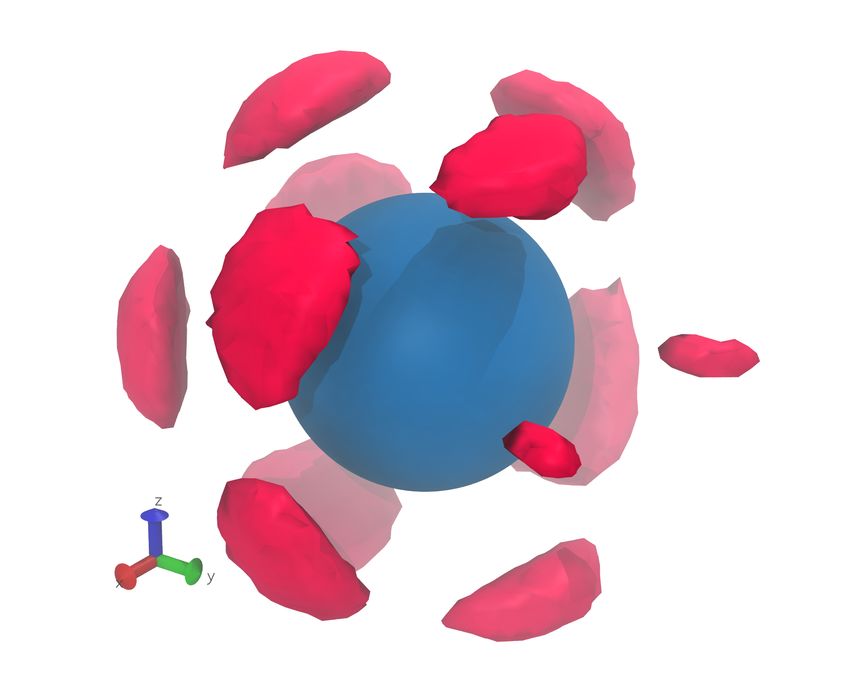
2

namic friction. This seminal idea pioneered by Born [19] has         successfully revealed two sequential structural transforma-
been successfully applied to salt solutions and developed by         tions of the water hydration shell with an increase in the
Boyd [20], Zwanzig [21], Onsager [22], Wolynes [23] and              ion electric field. An increase in the monopole-dipole in-
their coworkers. In the dielectric friction model, the total fric-   teraction induces the first transformation from a thick to a
tion ζ experienced by a spherical ion with charge q and radius       thin hydration shell. Its further increase leads to the sec-
R is given by                                                        ond transformation from radially disordered to ordered align-
                                                                     ments of water dipoles in the hydration shell, caused by the
                                ε0 − ε∞ τD q2 e2

              ζ = f1 ηR + f2                      .            (2)   monopole-dipole interaction overwhelming the water-water
                                   ε02       R3                      H-bonding and dipole-dipole interaction inside the hydration
                                                                     shell. Furthermore, in the regime of radial dipolar align-
   The first and second terms on the right side of this equa-
                                                                     ment, the dipolar-dipolar repulsion between water molecules
tion correspond to the hydrodynamic and dielectric friction,
                                                                     in a spherical shell leads to the high (low) orientational sym-
respectively. f1 and f2 are constants related to the boundary
                                                                     metry for a shell with a composite (prime) number of water
condition (stick or slip), η is the viscosity of the medium, ε0
                                                                     molecules inside, stabilizing (destabilizing) the water hydra-
and ε∞ are the low-frequency- and high-frequency-limit di-
                                                                     tion shell. We have revealed that these hydration shell struc-
electric constants, respectively, τD is the dielectric relaxation
                                                                     tures control ion dynamics and solvation stability. We have
time of the medium, and e is the elementary charge. The di-          also shown that our model nicely explains the experimentally
electric friction theory predicts that large ions follow Stokes’     observed dynamic behaviors of aqueous ionic solutions.
law (ζ ∝ R), whereas for small ions, the dielectric friction
(ζ ∝ R−3 ) is dominant. For example, this theory can explain
the slower diffusion of Li+ than Na+ in water even though Li+
is smaller than Na+ . Although the dielectric friction concept       Structural transition of hydration shell: translational ordering
successfully incorporates ion-dipole interactions with hydro-
dynamics and captures the essential physics of solvation, it             A cation attracts water molecules via the Coulomb inter-
treats the solvent as a continuum medium, neglecting the mi-         action to form (layered) spherical shells of solvent molecules
croscopic aspects of solvent-solvent (water-water H-bonding)         around it. The spherical shells are usually called hydration
and ion-solvent (monopole-dipole) interactions. Therefore,           shells, which are observed as peaks in the cation-oxygen ra-
the theory suffers from intrinsic difficulties in describing the     dial distribution function (RDF), g(r). Hereafter, we specifi-
solvent dynamics and the specificity of salt effects in aqueous      cally use the term “hydration shell” to refer to the first hydra-
solutions. We note that a continuum description is quite help-       tion shell closest to the cation, which is most strongly influ-
ful to understand macroscopic phase behaviors such as phase          enced by the solvation of ion [32]. The radius d of the hydra-
separation [24].                                                     tion shell is determined as the first peak position of g(r), and
   This article studies the solvation of a spherical ion in liq-     the coordination number n is defined as the number of water
uid water and its effect on solvent dynamics at the micro-           molecules in the hydration shell of the cation. Hereafter we
scopic level by molecular dynamics simulations (see supple-          use the hydration shell radius d instead of the VDW radius R
mentary material for the details). We utilized a newly devel-        to characterize the ion size since d is experimentally acces-
oped non-polarizable force field [25] for a series of aqueous        sible and directly determines the interaction between the ion
solutions based on a realistic TIP4P/2005 water model [26]           and water molecules in the hydration shell. Figure 1(a) shows
that has been shown to accurately describe the structure and         the contour map of n for cations with charge q 6 1.2 e. We can
dynamics of liquid water [27]. Starting from this potential,         see that a cation with a small charge typically has a large coor-
we continuously modified the van der Waals (VDW) radius              dination number n > 12. However, n dramatically drops to 4-
R and charge q of cation while keeping the force field pa-           8 as q increases, suggesting a sharp structural transformation
rameters fixed for the anion and TIP4P/2005 water. We have           of the hydration shell. Along an iso-ion-size line (the green
performed a high-throughput computational scanning of 1332           dashed curve in Fig. 1(a), on which the VDW radius of cation
model cations with different sizes and charges, covering the         R is kept constant), n shows a sharp drop from ∼ 14 to ∼ 6 at
alkali metal ions, the alkaline metal ions, and the IIIA-group       a transition point qs = 0.4 e with increasing q (Fig. 1(b)). Fig-
metal ions. This allows us to systematically study the salt ef-      ure 1(c) and Figs. S1-S2 show the typical cation-oxygen RDF,
fects in aqueous solutions with microscopic details beyond the       g(r), along the iso-ion-size line. Below qs , the cation has a
continuum theory. We emphasise here that continuous change           broad yet asymmetric hydration shell peak, whereas, above
of R and q is crucial for revealing a transitional nature of the     it, a narrow, symmetric hydration-shell peak is formed around
solvation state. Although the dispersion energy may affect the       the cation. Moreover, the second peaks are out-of-phase be-
salt effects as well [28, 29], here we focus on the effects of       tween cations with q > qs and q < qs , and the peaks other than
ion size and charge that directly determine the intensity of ion     the first peak fade away just around the transition, qs = 0.4 e.
electric field and thus the strength of dielectric friction. To      Such behavior is also captured by a translational order param-
minimize ion-ion interactions such as ion pairing [30] and co-       eter t of the solvent [33] (see supplementary material). As
operativity effects [31] that were activated in cencentrated so-     shown in Fig. 1(d), as q increases, t first decreases and then
lutions, here we constrain our study in a dilute concentration       increases substantially, showing a minimum at the transition
(∼ 0.16 mol/kg), focusing on ion-water interactions.                 point qs , in agreement with the structural features shown in
   From the high-throughput scanning of R and q, we have             Fig. 1(c).
3

               (a)                                                         (b)
                                                                               16
                                                                               14
                                                                               12

                                                                           n
                                                                               10
                                                                                8
                                                                                 6
                                                                                 4
                                                                                      0 0.2 0.4 0.6 0.8 1 1.2
               (c)                                                         (d)                 q (e)
                         6                                                    0.7
                                                        q=0
                         5                              q = 0.4
                                                                              0.6
                         4                              q = 0.8
                 g (r)

                                                                          t
                         3                                                    0.5
                         2
                         1                                                    0.4
                         0
                          1    2       3      4 5           6       7                 0 0.2 0.4 0.6 0.8 1 1.2
                                             r (Å)                                             q (e)
Fig. 1. Structural transition of the hydration shell. We measure the the number of water molecules in the hydration shell, n, and the radius of the
hydration shell, d, around cations of charge q. The radius d is defined as the first peak position in the cation-oxygen radial distribution function
(RDF). (a) The contour map of n shown as a function of d and q. The color bar represents the value of n. (b-d) The cationic coordination
number n (b), the cation-oxygen RDF g(r) (c), and the translational order parameter t of the cationic hydration shell (d) along the green dashed
line in panel a, along which the VDW size of the cation is kept constant. In (b) and (d), the cationic charge is increased from q = 0 to q = 1.2 e
with a step of 0.05 e.

   Not only the ion-water distance but also the water-ion-water                This breakdown of H-bonds by dipolar ordering is critical
angle in the hydration shell are regulated to increase the de-              for another structural transition in the hydration shell (see be-
gree of order as the ionic charge increases (Fig. S3). To under-            low). These results demonstrate that the solvation of a (nearly)
stand the mechanism of such behavior, we have simulated an                  neutral particle is intrinsically different from that of an ion.
ensemble of 50 non-equilibrium trajectories. Started from 50                Below the transition (q < qs ), an ion is solvated by a large
independent configurations equilibrated for q = 0.17 e < qs ,               number of solvent molecules with disordered arrangements.
we first jump the value of q instantaneously to 0.68 e > qs at              Since the ion does not perturb the solvent structure strongly,
time 0 and then monitored the structural evolution with time.               its dynamics can be described by Stokes law. Above the
The results are shown in Figs. S4 and S5. We can see that the               transition, the dielectric friction mechanism originating from
structural transformation starts with the orientational ordering            dipolar ordering should play a critical role in ion dynamics.
of water dipole in the hydration shell along the radial direc-              Therefore, we consider that the regimes below and above the
tion at a time scale of ∼ 0.03 ps. This process is accompanied              transition should correspond to the Stokes and dielectric fric-
by the breakdown of H-bonds and the bifurcation of the first                tion regimes, respectively [34].
g(r) peak of the hydration shell. This time scale corresponds
to the librational mode of a water molecule. The rotational
time correlation function in bulk water indicates that the li-                                       Dynamic crossover
bration mode couples with a reorientation of ∼ 23 ◦ of water
dipole at ∼ 0.03 ps (Fig. S4), leading to the breakdown of H-                  The solvent dynamics should be controlled by the size
bonds in water. Thus, we reveal that the coupling between                   and charge of ions. Figures 2(b) and (c) show the diffusion
ion-induced dipolar ordering and the libration mode breaks                  coefficient D1 and the residence time τres of hydrated wa-
the H-bonds and induces the structural reorganization of the                ter molecules (see Fig. 2(a) and supplementary material for
hydration shell.                                                            the explanation). Clearly, the dynamics of hydrated water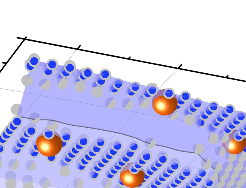
4

       (a)                              (b)                                                 (c)

                              Dw
                    dw

                  q+

Fig. 2. Crossover of solvent dynamics near a spherical ion. (a) Schematic illustration of the definition of τB and τres . The Brownian time
τB is defined as the time for a water molecule to diffuse over a distance of its diameter: τB = dw        2 /6D . Here D is the diffusion coefficient
                                                                                                                w           w
of a water molecule in bulk, and dw is the diameter of a water molecule that is obtained from the first peak position of the oxygen-oxygen
RDF of bulk water. The residence time τres is defined as the characteristic time for the hydrated water to leave the hydration shell of a cation
(see supplementary material). (b) The ratio D1 /Dw in the q-d plane. Here, D1 is the diffusion coefficient of a water molecule in the vicinity
of the hydration shell of a cation (see supplementary material). The color bar represents the value of D1 /Dw . (c) The logarithm of the ratio
τres /τB , log(τres /τB ), plotted in the q-d plane. The color bar represents the value of log(τres /τB ). In (b) and (c), the circle and square symbols
correspond to the dynamic crossover lines, for whose (q, d) D1 = Dw and τres = τB are satisfied, respectively.

molecules is slower under a stronger electrical field, i.e., for              ing to accelerated water dynamics. Based on this consider-
cations with larger q and smaller d. Here we scale D1 and τres                ation, we compare the dynamic crossover line with the con-
by the diffusion coefficient of bulk water Dw and the Brownian                dition of ∆Eion−water = EH−bond and find that they coincide
time of bulk water τB (the time for a water molecule in bulk to               well with each other within errors (see Fig. 3(b)). Moreover,
diffuse over a distance of its diameter), respectively. Then, the             the dynamic crossover line also coincides with the structural
two scaled variables exhibit similar dynamic crossover behav-                 transformation from an H-bonded to a non-H-bonded hydra-
iors from the accelerated to decelerated dynamics in the q − d                tion shell (Fig. 3(c)). This finding encourages us to introduce a
diagram (compare Figs. 2(b), (c)). This can be seen clearly in                new length λHB (q), which satisfies ∆Eion−water [d = λHB (q)] =
Fig. 3(b), which plots the dynamic crossover lines (D1 = Dw                   EH−bond . This characteristic length λHB (q) over which wa-
and τres = τB ) in the q − d diagram, together with a contour                 ter behaves water-like relatively free from ions naturally ex-
map of the ion-water interaction energy ∆Eion−water (q, d) (see               plains the dynamic crossover in aqueous solutions with spher-
Fig. 3(a) for the explanation of ∆Eion−water ). Remarkably, the               ical ions. This length λHB (q) may play a crucial role in our
dynamic crossover lines of the two dynamic quantities almost                  understanding of solvated water, as the Debye length λD and
coincide with each other in the q − d diagram, suggesting a                   the Bjerrum length λB do in the charge-related solution prob-
common physical mechanism behind their relative behaviors                     lem.
of the two quantities.

   In bulk water, water molecules tend to form an H-bond net-
work, whose strength EH−bond determines the dynamics of                            Orientational symmetry breaking of the hydration shell:
water. Adding ions to water introduces ion-water interac-                                           Polyhedral ordering
tion ∆Eion−water (q, d), which competes with the water-water
H-bonding to form hydration shells around ions. The hy-                          For d < λHB (q), we can see the nonmonotonic dependence
drated water under these competing interactions can have dy-                  of the dynamic properties on q and d (Figs. 2(b), (c)), e.g.,
namics distinct from the bulk water. If ∆Eion−water > EH−bond ,               specific regions with ultralong residence time (τres /τB > 103 )
the hydrated water should be dominated by the strong ion-                     in the q − d diagram. This suggests the formation of a sta-
water interaction rather than water-water H-bonding, leading                  ble hydration shell (Fig. 2(c)) for a specific combination of
to strong binding of water molecules to ions while breaking                   q and d. Further analysis reveals that the regions of stable
H-bonds (see Fig. 3(c)). This strong water binding to ions                    hydration correspond to the plateaus of the coordination num-
should slow down the ion motion, i.e., decelerated ion dy-                    ber n (Fig. 4(a)). In the q − d range of this study, we find
namics. On the other hand, if ∆Eion−water < EH−bond , the hy-                 that such plateaus emerge only when n is a composite number,
dration energy should be too weak to compete with the water-                  i.e., n = 4, 6, 8, 9, 10, and 12, whereas the hydration structure
water H-bonding, but the presence of ions should still per-                   of a prime coordination number is unstable, or even hard to
turb the water’s H-bond network. Although hydrated water                      form. A similar prime-number effect has been reported in the
molecules may remain H-bonded (Fig. 3(c)), the average H-                     Thomson problem that considers the most stable configura-
bond number and the H-bond strength are both reduced sta-                     tion of n point charges on a sphere with an opposite charge:
tistically (Fig. S7). Thus, the hydrated water tends to escape                In the range of n 6 30, Glasser and Every found that con-
from the ion and form new H-bonds with bulk water, lead-                      figurations with prime n show instability, whereas those with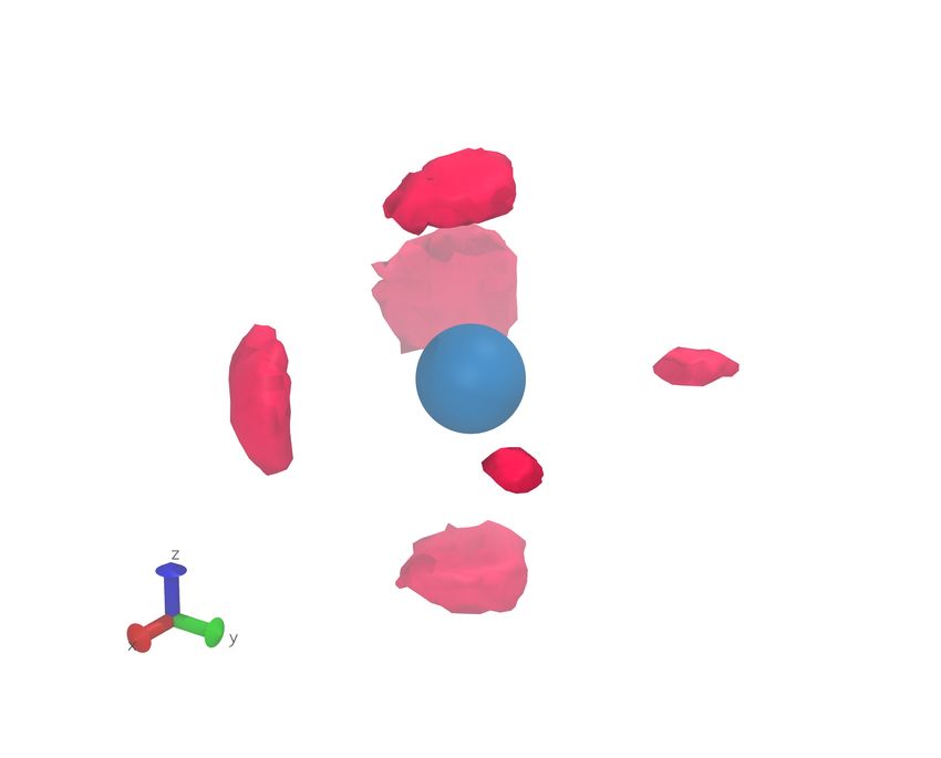
5
(a) q+
(b) ΔEion-water
U 1:
EH-bond
d
U 0:
q+
ΔEion-water = U1-U0
(c)
No
H-bonded?
Yes
Fig. 3. Ion-water interaction versus water-water hydrogen bonding upon solvation. (a) Schematic illustration of the definition of the excess
ion-water interaction energy ∆Eion−water (q, d) = U1 − U0 , where U1 is the interaction energy between an ion and a randomly oriented water
molecule, and U0 is the interaction energy between an ion and a water molecule in the lowest-energy water orientation, for a given charge of
an ion q and a given ion-oxygen distance d. (b) The contour map of ∆Eion−water (in the unit of kJ/mol). The dynamic crossover lines (symbols,
reproduced from Fig. 2) coincide well with the water-water H-bonding energy EH−bond (yellow band) in bulk water. The width of the yellow
HW−HW
band denotes the range of EH−bond under thermal fluctuations (Fig. S6). (c) The contour map of the average number of H-bonds NH−bond
HW−HW
between a hydrated water molecule and other water molecules within the same hydration shell. The color bar represents the value of NH−bond .
The dynamic crossover lines (symbols) coincide well with the crossover from H-bonded to non-H-bonded hydration shell. The left two panels
are schematic illustrations of H-bonded and non-H-bonded hydration shells of a cation.
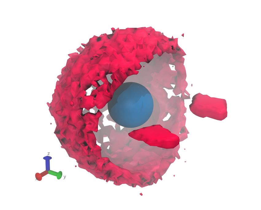
composite n are stable [35]. The similarity of ion hydration gions (Figs. 4(e), (f) ,(g)). These hydration shell structures are
to the Thomson problem can be explained by the fact that wa- markedly different from the nearly homogeneous shell struc-
ter dipoles in the hydration shell should align radially under tures in the non-plateau regions (Fig. S8). We also show the
strong enough electrostatic interaction from the central ion distribution of the oxygen-cation-oxygen angle φ in Fig. 4(c).
and repel each other on the ion surface, similar to the behavior As n increases, the smallest angle φ1 (i.e., the primary peak
of point charges of the same sign constrained on a spherical position of P(φ )) takes characteristic values that follow the
shell. solution φT of the Thomson problem (Fig. 4(d)). The lo-
The emergence of the stable hydration shell with composite cal orientational symmetry breaking in the plateau region at
n is associated with the orientational symmetry breaking of the composite number n explains the high stability of the hydra-
hydration shell. Figure 4(b) plots the cation-oxygen RDFs for tion shell, the ultralong residence time of water in the hydra-
typical cations in the plateau region (see big magenta spheres tion shell, and the slow solvent dynamics in the plateau re-
in Fig. 4(a)). Every RDF shows a sharp first peak and a well- gions (Fig. 2(b),(c)). We emphasise that the continuum the-
separated second shell (the first minimum goes to zero), in- ory can hardly capture this unique behavior originating from
dicating the local breaking of translational symmetry in the the molecular-level water-water interactions under the electric
stable hydration shell. Moreover, we find that the spatial dis- field of ions.
tributions of hydrated water molecules exhibit unique orien-
tational symmetries, such as tetrahedral (n = 4), octahedral
(n = 6) and icosahedral (n = 12) symmetry in the plateau re-6
(a) (b) (e)
12
10
9
8
6
4
(c) (f)
(d) (g)
Fig. 4. Orientational symmetry breaking of the hydration shell. (a) The coordination number n of a cation plotted in the q-d plane. The plateaus
of n highlighted by blue spheres indicate the formation of stable hydration shells. (b-c) The cation-oxygen RDF g(r) (b) and the distribution
of the oxygen-cation-oxygen angle P(φ ) (c) for typical cations in the plateau region of n = 4, 6, 8, 9, 10, and 12 (big magenta spheres in (a)).
The dash lines in (b) represent the coordination number of cations. The inset in (c) illustrates the definition of φ as the angle formed between
the cation and two water oxygen atoms in the hydration shell. The arrows in (b) and (c) denote the corresponding coordination number n of the
cation. (d) The relationship between the smallest angles φ1 for the primary peak of P(φ ) and the solution of the Thomson problem, φT [36].
The line has a slope of 1, suggesting φ1 = φT . (e-g) Spatial distribution of water molecules around a central ion with tetrahedral (e), octahedral
(f), and icosahedral (g) symmetries. The size of the central ion does not represent its actual size.
Comparison with experiments ter molecules and the development of translational order in
the radial direction. There is another transition in the dielec-
To compare our simulation results with real solutions, we tric friction regime due to the competition between ion-water
collected experimental data of the coordination number n and (monopole-dipole) electrostatic interaction and water-water
ion-water distance d (Table S1) for alkali, alkaline, and alu- H-bonding. This transition is accompanied by the dynamic
minium ions. We can see from Fig. 5(a)) that our model pre- transition of the solvent from the accelerated (B < 0) to de-
diction agrees well with the experimental data. In Fig. 5(b), celerated (B > 0) behavior. We also find that this transition
we plot the experimental B-coefficient in the q − d diagram. is characterized by a new characteristic length λHB (q), which
We can see in the diagram that the λHB line indeed separates marks the distance from the ion beyond which the electrostatic
kosmotropic (B > 0) and chaotropic (B < 0) ions. The struc- interaction does not significantly perturb the H-bonding.
ture maker/breaker classification has so far been made empiri- We also discover the orientational ordering of water dipoles
cally based on the sign of the B-coefficients [16, 17]. The crit- around ions in the hydration shell for a combination of q and
ical length λHB is determined by the competition of ion-water d in the higher q or lower d regime. This local orientational
and water-water interactions, providing new microscopic in- ordering is accompanied by a drastic increase in hydration
sight into the sign of the B-coefficient. Furthermore, we find shell stability and the residence time of water in the hydra-
that the quantity n∆Eion−water that measures the average ion- tion shell [38]. This ordering and stabilization of the hydra-
water interaction energy of n hydrated water molecules cor- tion shell occurs for a composite number of the hydrated wa-
relates well with the experimental B-coefficients of ions (Fig- ter molecules and does not for a prime number. We have re-
ure 5(c)). Our results confirm that both structure maker and vealed that the physics behind this unique ordering in a spher-
breaker perturb the water structure, in agreement with previ- ical shell is essentially the same as that of the Thomson prob-
ous scattering experiments [16]. lem of electrons around positive nucleus: repulsion-induced
ordering in the spherical shell.
We have summarized our main results in Table 1. All these
Conclusion and outlook discoveries were made possible only by a microscopic under-
standing of the structure of the water around the ions, which
We have revealed a structural transition of the hydration is not possible with the continuum theory. We hope that this
shell in the q − d space, accompanied by the crossover from work will contribute to the development of microscopic theo-
the Stokes to the dielectric friction regime with an increase in ries of solvation around spherical ions.
the electric field of ions, which is realized for ions of stronger This work provides a simple physical picture of salt effects
charge and/or smaller size. This structural transition is sharp on water, based on the classical description of the electro-
and accompanied by the significant reduction of hydrated wa- static and VDW interactions. Our approach may be consid-7
(a) (b) (c) 1.4
1.2
3+
0.91 1
B (dm3mol-1)
0.8
0.6 2+
Ba2+ 0.39 0.39 0.28 0.26 0.22
2+
Cs+
Rb+
0.4 1+
Sr
K+
Ca2+ Na+ -0.05
0.2
Mg2+ 0.15 0.09 -0.01 -0.03 0
Al3+ Li+ -0.2
Be2+ -0.4
0 500 1000
n ΔEion-water
Fig. 5. The “phase diagram” of the hydration shell around spherical ions in water. (a) The coordination number n of cationic ions obtained from
experimental data (big spheres) and our model (small blue spheres and red cubes). (b) The q − d “phase diagram” of aqueous ionic solutions.
The experimental B-coefficient [37] in the unit of dm3 mol−1 at 298.15 K is shown for each ion. The solid line indicates the H-bonding energy
scale, separating B > 0 (orange circles) with B < 0 (violet squares) ions. The dashed line represents the transition line from the Stokes (red
shaded region) to the dielectric regime (blue shaded region). (c) The correlation between the B-coefficient experimentally estimated and the
ion-water interaction energy in the hydration shell n∆Eion−water . Red circles and blue squares represent the data for alkali metal ions and
alkaline metal ions, respectively, and diamond denotes the aluminium ion. Among the same symbol, the darker one represents the bigger ion.
Table 1. Classification of the ion hydration states and dynamic characteristics.
Electrical field Hydration Water structure Friction B Water dynamics
on ion surface shell (HS) around ion coefficient in HS
weak thick disordered viscous B∼0 comparable to bulk
H-bonding in HS (Stokes)
intermediate low translational order weakly accelerated
d > λHB weak radial alignment of dipoles B0 --------------------
composite n: dielectric longer residence time
water polyhydral ordering slower water diffusion
(compared with prime n)
----------------------- --------------------
prime n: shorter residence time
no polyhedral order faster water diffusion
(compared with composite n)
ered as a zero-order approximation for such complex effects.
Higher-order effects, such as polarizability, many-body inter-
actions, and nuclear quantum effects, would be necessary for
a more precise and comprehensive description of ion-specific
effects in aqueous solutions. Moreover, this study has con-
sidered only hydration around spherical ions, but solvation
around molecular ions with complex shapes is an important
topic for future research. We expect the characteristic length
λHB and prime-number effect introduced here to be helpful in
these cases as well.
This study was partly supported by Specially Promoted
Research (JP20H05619 and JP25000002) and Scientific Re-
search (A) (JP18H03675) from the Japan Society for the Pro-
motion of Science (JSPS) and the Mitsubishi Foundation.8
[1] R. W. Gurney, Ionic processes in solution (McGraw-Hill, 1953). [22] J. Hubbard and L. Onsager, Dielectric dispersion and dielec-
[2] E. R. Nightingale Jr, Phenomenological theory of ion solvation. tric friction in electrolyte solutions. I., J. Chem. Phys. 67, 4850
Effective radii of hydrated ions, J. Phys. Chem. 63, 1381 (1959). (1977).
[3] P. Ball, Water as an active constituent in cell biology, Chem. [23] P. G. Wolynes, Molecular theory of solvated ion dynamics, J.
Rev. 108, 74 (2008). Chem. Phys. 68, 473 (1978).
[4] H. J. Bakker, Structural dynamics of aqueous salt solutions, [24] A. Onuki, T. Araki, and R. Okamoto, Solvation effects in phase
Chem. Rev. 108, 1456 (2008). transitions in soft matter, J. Phys.: Condens. Matter 23, 284113
[5] Y. Marcus, Effect of ions on the structure of water: structure (2011).
making and breaking, Chem. Rev. 109, 1346 (2009). [25] I. M. Zeron, J. L. F. Abascal, and C. Vega, A force field of Li+ ,
[6] A. Hudait and V. Molinero, Ice crystallization in ultrafine Na+ , K+ , Mg2+ , Ca2+ , Cl− , and SO2− 4 in aqueous solution
water–salt aerosols: Nucleation, ice-solution equilibrium, and based on the TIP4P/2005 water model and scaled charges for
internal structure, J. Am. Chem. Soc. 136, 8081 (2014). the ions, J. Chem. Phys. 151, 134504 (2019).
[7] M.-C. Bellissent-Funel, A. Hassanali, M. Havenith, R. Hench- [26] J. L. F. Abascal and C. Vega, A general purpose model for the
man, P. Pohl, F. Sterpone, D. van der Spoel, Y. Xu, and A. E. condensed phases of water: TIP4P/2005, J. Chem. Phys. 123,
Garcia, Water determines the structure and dynamics of pro- 234505 (2005).
teins, Chem. Rev. 116, 7673 (2016). [27] C. Vega, J. L. F. Abascal, M. M. Conde, and J. L. Aragones,
[8] S. Mukherjee, S. Mondal, and B. Bagchi, Mechanism of sol- What ice can teach us about water interactions: a critical com-
vent control of protein dynamics, Phys. Rev. Lett. 122, 058101 parison of the performance of different water models, Faraday
(2019). Discuss. 141, 251 (2009).
[9] T. Koop, B. Luo, A. Tsias, and T. Peter, Water activity as the de- [28] M. Andreev, A. Chremos, J. de Pablo, and J. F. Douglas,
terminant for homogeneous ice nucleation in aqueous solutions, Coarse-grained model of the dynamics of electrolyte solutions,
Nature 406, 611 (2000). J. Phys. Chem. B 121, 8195 (2017).
[10] G. D. Soria, J. R. Espinosa, J. Ramirez, C. Valeriani, C. Vega, [29] M. Andreev, J. J. de Pablo, A. Chremos, and J. F. Douglas, In-
and E. Sanz, A simulation study of homogeneous ice nucleation fluence of ion solvation on the properties of electrolyte solu-
in supercooled salty water, J. Chem. Phys. 148, 222811 (2018). tions, J. Phys. Chem. B 122, 4029 (2018).
[11] M. M. Conde, M. Rovere, and P. Gallo, Molecular dynamics [30] N. F. Van Der Vegt, K. Haldrup, S. Roke, J. Zheng, M. Lund,
simulations of freezing-point depression of TIP4P/2005 water and H. J. Bakker, Water-mediated ion pairing: Occurrence and
in solution with NaCl, J. Mol. Liq. 261, 513 (2018). relevance, Chem. Rev. 116, 7626 (2016).
[12] Y. Liu, T. Lafitte, A. Z. Panagiotopoulos, and P. G. Debenedetti, [31] K. Tielrooij, N. Garcia-Araez, M. Bonn, and H. Bakker, Coop-
Simulations of vapor–liquid phase equilibrium and interfacial erativity in ion hydration, science 328, 1006 (2010).
tension in the CO2 –H2 O–NaCl system, AIChE J. 59, 3514 [32] A. W. Omta, M. F. Kropman, S. Woutersen, and H. J. Bakker,
(2013). Negligible effect of ions on the hydrogen-bond structure in liq-
[13] G. Gonella, E. H. Backus, Y. Nagata, D. J. Bonthuis, P. Loche, uid water, Science 301, 347 (2003).
A. Schlaich, R. R. Netz, A. Kühnle, I. T. McCrum, M. T. Koper, [33] J. R. Errington and P. G. Debenedetti, Relationship between
M. Wolf, B. Winter, G. Meijer, R. K. Campen, and M. Bonn, structural order and the anomalies of liquid water, Nature 409,
Water at charged interfaces, Nat. Rev. Chem. 5, 466 (2021). 318 (2001).
[14] J. Peng, D. Cao, Z. He, J. Guo, P. Hapala, R. Ma, B. Cheng, [34] F. Martelli, R. Vuilleumier, J.-P. Simonin, and R. Spezia, Vary-
J. Chen, W. J. Xie, X.-Z. Li, P. Jelínek, L.-M. Xu, E.-G. Wang, ing the charge of small cations in liquid water: Structural,
and Y. Jiang, The effect of hydration number on the interfacial transport, and thermodynamical properties, J. Chem. Phys. 137,
transport of sodium ions, Nature 557, 701 (2018). 164501 (2012).
[15] G. Jones and M. Dole, The viscosity of aqueous solutions of [35] L. Glasser and A. G. Every, Energies and spacings of point
strong electrolytes with special reference to barium chloride, J. charges on a sphere, J. Phys. A-Math. Gen. 25, 2473 (1992).
Am. Chem. Soc. 51, 2950 (1929). [36] T. Erber and G. M. Hockney, Equilibrium configurations of N
[16] R. Mancinelli, A. Botti, F. Bruni, M. A. Ricci, and A. K. Soper, equal charges on a sphere, J. Phys. A-Math. Gen. 24, L1369
Hydration of sodium, potassium, and chloride ions in solution (1991).
and the concept of structure maker/breaker, J. Phys. Chem. B [37] H. D. B. Jenkins and Y. Marcus, Viscosity B-coefficients of ions
111, 13570 (2007). in solution, Chem. Rev. 95, 2695 (1995).
[17] P. Gallo, D. Corradini, and M. Rovere, Ion hydration and struc- [38] Y. Lee, D. Thirumalai, and C. Hyeon, Ultrasensitivity of water
tural properties of water in aqueous solutions at normal and su- exchange kinetics to the size of metal ion, J. Am. Chem. Soc.
percooled conditions: a test of the structure making and break- 139, 12334 (2017).
ing concept, Phys. Chem. Chem. Phys. 13, 19814 (2011). [39] Z. R. Kann and J. L. Skinner, A scaled-ionic-charge simulation
[18] H. Tanaka, H. Tong, R. Shi, and J. Russo, Revealing key struc- model that reproduces enhanced and suppressed water diffusion
tural features hidden in liquids and glasses, Nat. Rev. Phys. 1, in aqueous salt solutions, J. Chem. Phys. 141, 104507 (2014).
333 (2019). [40] B. Hess, C. Kutzner, D. Van Der Spoel, and E. Lindahl, GRO-
[19] M. Born, Über die beweglichkeit der elektrolytischen ionen, Z. MACS 4: algorithms for highly efficient, load-balanced, and
Phys. 1, 221 (1920). scalable molecular simulation, J. Chem. Theory Comput. 4, 435
[20] R. H. Boyd, Extension of Stokes’ law for ionic motion to in- (2008).
clude the effect of dielectric relaxation, J. Chem. Phys. 35, 1281 [41] A. H. Narten, F. Vaslow, and H. A. Levy, Diffraction pattern and
(1961). structure of aqueous lithium chloride solutions, J. Chem. Phys.
[21] R. Zwanzig, Dielectric friction on a moving ion. II. Revised 58, 5017 (1973).
theory, J. Chem. Phys. 52, 3625 (1970). [42] J. Mähler and I. Persson, A study of the hydration of the alkali9
metal ions in aqueous solution, Inorg. Chem. 51, 425 (2012).
[43] T. Yamaguchi, H. Ohtaki, E. Spohr, G. Palinkas, K. Heinzinger,
and M. M. Probst, Molecular dynamics and X-ray diffraction
study of aqueous beryllium (II) chloride solutions, Z. Natur-
forsch. A 41, 1175 (1986).
[44] R. Caminiti, G. Licheri, G. Piccaluga, and G. Pinna, X-ray
diffraction study of MgCl2 aqueous solutions, J. Appl. Cryst.
12, 34 (1979).
[45] F. Jalilehvand, D. Spångberg, P. Lindqvist-Reis, K. Hermans-
son, I. Persson, and M. Sandström, Hydration of the calcium
ion. An EXAFS, large-angle X-ray scattering, and molecular
dynamics simulation study, J. Am. Chem. Soc. 123, 431 (2001).
[46] R. H. Parkman, J. M. Charnock, F. R. Livens, and D. J.
Vaughan, A study of the interaction of strontium ions in aque-
ous solution with the surfaces of calcite and kaolinite, Geochim.
Cosmochim. Acta 62, 1481 (1998).
[47] J. N. Albright, X-Ray diffraction studies of aqueous alkaline-
earth chloride solutions, J. Chem. Phys. 56, 3783 (1972).
[48] R. Caminiti, G. Licheri, G. Piccaluga, G. Pinna, and T. Radnai,
Order phenomena in aqueous AlCl3 solutions, J. Chem. Phys.
71, 2473 (1979).10
SUPPLEMENTARY MATERIAL the cation. The systems have the same number of cations and
anions to keep the charge neutrality.
METHODS Method for equilibrium simulations
Potentials for aqueous ionic solutions We have performed high-throughput molecular dynamics
It has been demonstrated that a realistic TIP4P/2005 wa- simulations of 1332 model solutions containing cations with
ter model [26] accurately describes the structural and dy- different sizes and charges. Simulations were performed us-
namic properties of liquid water [27]. Focusing on the wa- ing the Gromacs (v.4.6.7) simulation package [40] with a time
ter structure and dynamics, we employed a non-polarizable step of 2 fs. The system consists of 3456 water molecules, 10
force field [25] that was newly developed for aqueous salt so- cations, and some anions (from 2 to 40, determined by the
lutions, based on the TIP4P/2005 water model. This force charge neutrality condition) in a periodic cubic box. This cor-
field, compatible with the TIP4P/2005 water, shows reason- responds to a dilute concentration of ∼ 0.16 mol/kg of the
ably good performance for modelling a series of aqueous salt salt. We used the isothermal-isobaric NPT ensemble for all
solutions [25]. the simulations. We employed the Nose-Hoover thermostat
The size and charge of the ions together determine the ion- with a coupling time of 1.0 ps and an isotropic Parrinello-
solvent interactions. The intermolecular interaction V be- Rahman barostat with a coupling time of 2.0 ps to keep the
tween atoms i and j is given by the sum of VDW and Coulom- temperature at 300 K and pressure at 1 bar. The Particle-Mesh
bic potentials: Ewald method was applied for long-range electrostatic inter-
" 6 # actions. The VDW interactions and the Coulomb potential in
σi j 12 σi j 1 qi q j real space were cut at 10 Å. All the 1332 systems were first
V (ri j ) = 4εi j − + , (3)
ri j ri j 4πε0 ri j equilibrated for 0.3 ns and followed by a production run for
1 ns.
where ri j is the distance between atoms i and j, εi j is the en-
ergy scale of the VDW potential, σi j is the VDW diameter, Method for non-equilibrium simulations
ε0 is the vacuum permittivity, and qi and q j are the charges A high-throughput scanning in the charge-size space re-
of atoms i and j. The dielectric friction theory (equation (2)), vealed a structural transition of the ionic hydration shell in
which treats the solvent as the continuum media, has shown the small-fractional-charge region. In order to understand the
that the size and charge of an ion control dynamics of a given mechanism of the structural transition, we performed non-
solvent. In order to investigate the dependence of salt effects equilibrium molecular dynamics for a system containing 3456
on the ion size and charge, we employed the above-mentioned water molecules, 10 cations with σcation−O = 2.76 Å, and
force field parameters for aqueous NaCl solution as the ref- 8 chloride anion. For this system, the transition occurs at
erence and then continuously tuned the VDW size and the qs = 0.4 e. We first set the cation charge as q = 0.17 e below
charge of the cation, while the force field parameters being the transition threshold and equilibrated the system at 300 K
fixed for anion (Cl− ) and TIP4P/2005 water. Practically, we and 1 bar for 1.0 ns. Then, 50 independent configurations
linearly modified the VDW parameter σ between cation and were evenly sampled from 1-ns trajectories. We carried out 50
water oxygen (chloride) as σcation−O(Cl) = σNa−O(Cl) + k · δ σ , production runs using these configurations as the initial ones,
where k is an integer, δ σ is chosen to be 0.04 Å and σNa−O(Cl) at 300 K and 1 bar for 3 ps. Then, we jumped the charge of
is the VDW parameter in the original force field [25]. cations to q = 0.68 e at time 0 instantaneous to induce the tran-
In the original force field, the chloride ion has a reduced sition. The configurations were sampled every 4 fs to follow
charge of -0.75 e to include the polarizable effect effec- the transition kinetics. The charge of anions was adjusted to
tively [39]. Therefore, the cation charge is given by qcation = ensure charge neutrality. The other simulation details are the
k · δ q, where k is an integer and δ q is chosen as 0.85
5 = 0.17 e. same as the equilibrium simulations described above. Results
Then, the number of ions is adjusted to ensure the charge neu- obtained from these non-equilibrium simulations were aver-
trality of the system. In this way, we prepared potentials for aged over the 50 trajectories to reduce statistical fluctuations.
1332 model systems with cationic charge ranging from 0.17
to 3.4 e that covers most of the alkali metal ions, the alkaline Structural analysis tools
metal ions, and the IIIA-group metal ions. To characterize the hydration structure around ions, we in-
troduce the structural parameter t [33] as t = ξ1c 0 c |g (ξ ) −
Rξ
Potentials for aqueous ionic solutions with small fractional
charges 1|dξ , where g is the cation-oxygen RDF, ρ is the number
We scanned 20 points in the charge space using the poten- density of water, ξc = 2.843 is a cut-off distance. The pa-
tial mentioned above with a resolution of δ q = 0.17 e for a rameter t measures the degree of translational order of solvent
given cation size. In order to increase the resolution in the molecules around a cation in the radial direction.
small-fractional-charge region, we prepared 25 new systems
with the same VDW parameter σcation−O = 2.73 Å which is Dynamic analysis tools
close to the VDW parameter for the sodium ion. In the new The diffusion coefficient D1 characterizes the speed of
systems, the cation charge is varied from 0 to 1.2 e with a res- diffusive motion of a hydrated water molecule in the hy-
olution of δ q = 0.05 e, and the anion has the same charge as dration shell. The mean-squared displacement of wa-11
ter molecule i in the hydration shell of ion j at t =
0 can be calculated from the trajectory as MSD (t) =
h[~ri (t) −~ri (0)]2 δ [|~ri (0) −~r j (0) | − r1 ]i, where r1 is the char-
acteristic size of the hydration shell determined as the first
minimum position of the cation-oxygen RDF g(r), δ (x) = 1
if x 6 0 and δ (x) = 0 otherwise, h· · · i denotes the ensemble
average. The diffusion coefficient D1 is then obtained, us-
ing the Einstein relation, MSD = 6D1t, where an upper bound
MSD 6 16 Å is set to ensure the locality of D1 .
The residence time τR of a water molecule in the hydra-
tion shell can be characterized by the continuous time corre-
lation function, P (t) = h p(t)p(0)p(0) i, where p (t) = 1 if a water
molecule that is in the hydration shell of an ion at t = 0 con-
tinuously stays in the hydration shell of the same ion at time t;
otherwise, p (t) = 0. Then, the residence time can be extracted
from P (t), using the following equation, P (τR ) = e−1 . Here,
we regard a water molecule to remain in the hydration shell if
it is within a distance r1 from the central ion.
SUPPLEMENTARY FIGURES AND TABLES12
1 0 1 4
1 2
8
1 0
g (r)
6 8
n
4 6
q = 1 .2 4
2 2
0 0 0
1 2 3 4 5 6 7
r (Å )
Fig. S1. Ion-water (cation-oxygen) radial distribution function (RDF) in aqueous ionic solutions along the green dashed line in Fig. 1(a). In the
solutions, the cation charge is varied from q = 0 to q = 1.2 e with δ q = 0.05 e, while the VDW size of cations is fixed to σcation−O = 2.73 Å.
The RDF at the structural transition (qs = 0.4 e) is highlighted by the black thick line. The coordination number n is shown by dotted curves
(see the right axis for the value).13
3 3 3 3 3
0 0 .0 5 0 .1 0 .1 5 0 .2
2 2 2 2 2
g (r)
g (r)
g (r)
g (r)
g (r)
1 1 1 1 1
0 0 0 0 0
1 2 3 4 5 6 7 8 9 1 2 3 4 5 6 7 8 9 1 2 3 4 5 6 7 8 9 1 2 3 4 5 6 7 8 9 1 2 3 4 5 6 7 8 9
r (Å ) r (Å ) r (Å ) r (Å ) r (Å )
3 3 3 3 3
0 .2 5 0 .3 0 .3 5 0 .4 0 .4 5
2 2 2 2 2
g (r)
g (r)
g (r)
g (r)
g (r)
1 1 1 1 1
0 0 0 0 0
1 2 3 4 5 6 7 8 9 1 2 3 4 5 6 7 8 9 1 2 3 4 5 6 7 8 9 1 2 3 4 5 6 7 8 9 1 2 3 4 5 6 7 8 9
r (Å ) r (Å ) r (Å ) r (Å ) r (Å )
3 3 3 3 3
0 .5 0 .5 5 0 .6 0 .6 5 0 .7
2 2 2 2 2
g (r)
g (r)
g (r)
g (r)
g (r)
1 1 1 1 1
0 0 0 0 0
1 2 3 4 5 6 7 8 9 1 2 3 4 5 6 7 8 9 1 2 3 4 5 6 7 8 9 1 2 3 4 5 6 7 8 9 1 2 3 4 5 6 7 8 9
r (Å ) r (Å ) r (Å ) r (Å ) r (Å )
3 3 3 3 3
0 .7 5 0 .8 0 .8 5 0 .9 0 .9 5
2 2 2 2 2
g (r)
g (r)
g (r)
g (r)
g (r)
1 1 1 1 1
0 0 0 0 0
1 2 3 4 5 6 7 8 9 1 2 3 4 5 6 7 8 9 1 2 3 4 5 6 7 8 9 1 2 3 4 5 6 7 8 9 1 2 3 4 5 6 7 8 9
r (Å ) r (Å ) r (Å ) r (Å ) r (Å )
3 3 3 3 3
1 1 .0 5 1 .1 1 .1 5 1 .2
2 2 2 2 2
g (r)
g (r)
g (r)
g (r)
g (r)
1 1 1 1 1
0 0 0 0 0
1 2 3 4 5 6 7 8 9 1 2 3 4 5 6 7 8 9 1 2 3 4 5 6 7 8 9 1 2 3 4 5 6 7 8 9 1 2 3 4 5 6 7 8 9
r (Å ) r (Å ) r (Å ) r (Å ) r (Å )
Fig. S2. Individual ion-water (cation-oxygen) RDF in aqueous ionic solutions along the green dashed line in Fig. 1(a). The results are the
same as Fig. S1, but displayed separately.14
q = 1.2
0.06
0.04
P (φ )
φ
0.02
0
0
30 60 90 120 150 180
φ (degree)
Fig. S3. Probability distribution function of the oxygen-cation-oxygen angle φ , P(φ ), in aqueous ionic solutions along the green dashed line
in Fig. 1(a). The angle φ is defined as the angle formed between the cation and two neighboring water oxygen atoms in the hydration shell
(see inset). We varied the cation charge from q = 0 to q = 1.2 e with a step of δ q = 0.05 e, whereas the VDW size of cations was fixed to
σcation−O = 2.73 Å. P(φ ) at the structural transition (i.e., at qs = 0.4 e) is highlighted by the black thick line.15
(a) (b)
Fig. S4. Non-equilibrium structural transformation process in response to the instantaneous jump of cationic charge at time τ = 0. (a)
Schematic illustration of the definition of angle θ , which is the angle formed by the water dipole and the ion-oxygen vector. (b) The temporal
decay of the rotational time correlation function C2 (τ) = 1.5h~µ(τ)~µ(0)i2 − 0.5 of the water dipole moment ~µ as a function of time τ in bulk
TIP4P/2005 water. (c) Time evolution of hcos θ i for water molecules in the hydration shell of cations in response to the instantaneous jump
of the cation charge from q = 0.17 to 0.68 e at τ = 0. The VDW size of cations was fixed to σcation−O = 2.76 Å. The color bar represents the
value of hcos θ i.16 (a) (b) Fig. S5. Non-equilibrium structural transformation process in response to the instantaneous jump of cationic charge at time τ = 0. Time evolution of the ion-water RDF gion−water (r, τ) (a) and the H-bond number NH−bond per water molecule (b) in response to the instantaneous jum of cationic charge from q = 0.17 to 0.68 e at τ = 0. The color bars in panels a and b represent the height of gion−water and the value of NH−bond , respectively.
17

Fig. S6. Inter water H-bonding energy in bulk water. Probability distribution function of the H-bonding energy EH−bond in bulk TIP4P/2005
water at 300 K and 1 bar. The full width at half maximum, as shown by the arrow, indicates the range of fluctations of the H-bonding energy
in bulk water, which corresponds to the width of the yellow band in Fig. 3(b).
18

(a)                                                                    (b)

Fig. S7. Inter water H-bonding in hydration shell. (a) Average number of H-bonds formed for a water molecule in the hydration shell of
          HW
cation, NH−bond  . Here we consider all H-bonds formed for a hydrated water with other waters within and outside the same hydration shell.
                         HW−HW
This is different from NH−bond   , which only counts the number of H-bonds between a hydrated water molecule and other water molecules
                                                                                        HW
within the same hydration shell (see Fig. 3(c)). The color bar represents the value of NH−bond . Note that in bulk TIP4P/2005 water, each water
molecule forms 3.7 H-bonds on average at 300 K and 1 bar. (b) The energy difference between the H-bond formed by two hydrated water
                                                                                     HW−HW
in the hydration shell of the same cation and the H-bond formed in bulk water, EH−bond       − EH−bond . The color bar represents the value of
  HW−HW
EH−bond − EH−bond in the unit of kJ/mol.
19
z
y
x
Fig. S8. Orientational symmetry of a typical unstable hydration shell. Spatial distribution of water molecules around a cation with the
coordination number of n = 6. We can see that the distribution has a homogeneous angular distribution without the breakdown of orientational
symmetry. We note that this particular state point (the cation charge q = 0.51 e and the size of the hydration shell d = 2.6 Å) is located outside
of the plateau region of Fig. 4(a), and the hydration shell is not stable. Two neighboring water molecules are selected to determine the xyz axes
(two separated clouds on the right-handed side). The size of the ion in the centre does not represent the actual size of the ion.20
Table S1. The radius d of hydration shell and the coordination number n of cations in aqueous solutions obtained from experimental measure-
ments.
Cation Salt d (Å) n Method reference
Li+ LiCl 1.95 4.0 X-ray and Neutron Ref. [41]
Na+ NaI 2.43 6.0 X-ray Ref. [42]
K+ KI 2.81 7.0 X-ray Ref. [42]
Rb+ RbI 2.98 8.0 X-ray Ref. [42]
Cs+ CsI 3.081 8.0 X-ray Ref. [42]
Be2+ BeCl2 1.67 4.0 X-ray Ref. [43]
Mg2+ MgCl2 2.1 6.0 X-ray Ref. [44]
Ca2+ CaCl2 2.46 8.0 X-ray Ref. [45]
Sr2+ SrCl2 2.61 8.3 X-ray Ref. [46]
Ba2+ BaCl2 2.9 9.5 X-ray Ref. [47]
Al3+ AlCl3 1.902 6.0 X-ray Ref. [48]You can also read