Spatial eco-evolutionary feedbacks mediate coexistence in prey-predator systems
←
→
Page content transcription
If your browser does not render page correctly, please read the page content below
Spatial eco-evolutionary feedbacks mediate coexistence in
                                                           prey-predator systems
                                                           Eduardo H. Colombo1* , Ricardo Martı́nez-Garcı́a2, Cristóbal López1 , Emilio
                                                           Hernández-Garcı́a1

                                                           1 IFISC (CSIC-UIB), Campus Universitat Illes Balears, 07122, Palma de Mallorca,
arXiv:1902.03016v1 [q-bio.PE] 8 Feb 2019

                                                           Spain
                                                           2 Department of Ecology and Evolutionary Biology, Princeton University, Princeton
                                                           NJ 08544, USA

                                                           * ecolombo@ifisc-uib.csic.es

                                                           Abstract
                                                           Eco-evolutionary frameworks can explain certain features of communities in which
                                                           ecological and evolutionary processes occur over comparable timescales. In the
                                                           particular case of prey-predator systems, a combination of empirical and theoretical
                                                           studies have explored this possibility, showing that the evolution of prey traits,
                                                           predator traits or the coevolution of both can contribute to the stability of the
                                                           community, as well as to the emergence of various types of population cycles. However,
                                                           these studies overlook that interactions are spatially constrained, a crucial ingredient
                                                           known to foster species coexistence per se. Here, we investigate whether evolutionary
                                                           dynamics interacts with the spatial structure of a prey-predator community in which
                                                           both species show limited mobility and predators perceptual ranges are subject to
                                                           natural selection. In these conditions, our results unveil an eco-evolutionary feedback
                                                           between species spatial mixing and predators perceptual range: different levels of
                                                           species mixing select for different perceptual ranges, which in turn reshape the spatial
                                                           distribution of preys and their interaction with predators. This emergent pattern of
                                                           interspecific interactions feeds back to the efficiency of the various perceptual ranges,
                                                           thus selecting for new ones. Finally, since prey-predator mixing is the key factor that
                                                           regulates the intensity of predation, we explore the community-level implications of
                                                           such feedback and show that it controls both coexistence times and species extinction
                                                           probabilities.

                                                           Author summary
                                                           Evolutionary processes occurring on temporal scales that are comparable to those of
                                                           ecological change can result in reciprocal interactions between ecology and evolution
                                                           termed eco-evolutionary feedbacks. Such interplay is clear in prey-predator systems, in
                                                           which predation alters the distribution of resources (preys). In turn, changes in the
                                                           abundance and spatial distribution of preys may lead to the evolution of new
                                                           predation strategies, which may change again the properties of the prey population.
                                                           Here, we investigate the interplay between limited mobility, species mixing, and finite
                                                           perception in a prey-predator system. We focus on the case in which predator
                                                           perceptual ranges are subject to natural selection and examine, via coexistence times
                                                           and species extinction probabilities, whether the resulting eco-evolutionary dynamics

                                       February 11, 2019                                                                                      1/22
mediates the stability of the community. Our results confirm the existence of such
                    eco-evolutionary feedback and reveal its potential impact on community-level
                    processes.

                    Introduction
                    One of the major goals of ecology is to understand the mechanisms that sustain the
                    coexistence of antagonistic species, such as one prey and its predator or competitors
                    for common resources. Under the traditional assumption that ecological and
                    evolutionary changes occur on very different time scales, the connection between
                    ecology and evolution is unidirectional, with the former driving the later. Therefore,
                    the first attempts to explain species coexistence neglected the role of evolutionary
                    processes and relied exclusively on ecological factors, such as species neutrality [1],
                    frequency-dependent interactions [2], and environmental heterogeneity, either in space
                    or in time [3–7].
                        More recently, however, evidences that ecological and evolutionary processes can
                    occur at congruent time-scales have been found [8–10]. This result suggests that both
                    processes can affect each other in some situations and establish ‘eco-evolutionary
                    feedbacks’ (EEFs) that may alter the ecological dynamics and the stability of
                    communities. Due to rapid evolution, the frequency of the genotypes and their
                    associated phenotypes within a population changes as fast as ecological variables, like
                    population sizes or spatial distributions, and affect their dynamics. In turn, these new
                    ecological configurations redirect the evolutionary process [11–16].
                        The consequences of these EEFs at the community level have been studied mainly
                    in single-species populations and simple two-species communities [13]. In
                    prey-predator systems, empirical studies have shown that both prey and predator
                    traits can evolve over ecological time scales, leading to EEFs that alter some features
                    of the dynamics of the populations [17, 18]. For instance, in a rotifer-algal system,
                    rapid prey evolution induced by oscillatory predator abundance can drive antiphase in
                    prey-predator cycles [14]. Theoretical investigations have also suggested that
                    prey-predator coevolution can induce a rich set of behaviors in population abundances,
                    including reversion in the predator-prey cycles [19]. Another family of studies has
                    focused on the role of EEFs on the stability of the community, showing that different
                    feedbacks influence the stability of prey-predator dynamics in different ways
                    depending on the shape of the trade-offs between the evolving traits [13, 20, 21].
                        However, despite these insightful studies, the interplay between eco-evolutionary
                    feedbacks and spatial dynamics, a crucial aspect that often controls species
                    interactions, remains largely unexplored in prey-predator systems. EEFs in spatially
                    structured populations have been studied mostly for single-species populations in
                    which evolutionary dynamics affects the rate of dispersal, either across patches or
                    during range expansions [13, 22, 23]. Here, we extend those scenarios and investigate
                    how eco-evolutionary dynamics can modulate two-species interactions in a
                    spatially-extended prey-predator community. To this aim, we use an individual-based
                    model in which both species have limited mobility and predation is nonlocal, i.e., only
                    preys within a finite region around the predator are susceptible to predation. The
                    radius of this region defines predators perceptual range, which in our model varies
                    across the population and is subject to natural selection. Perceptual ranges, generally
                    defined as the maximum distance at which individuals can identify elements of the
                    landscape, vary tremendously within species and have a strong impact on determining
                    the success of foraging and haunting strategies via several trade-offs [24, 25]. For
                    instance, large perceptual ranges increase the number of potentially detectable preys,
                    but may lead to a reduced attacking efficiency, as information is integrated over a

February 11, 2019                                                                                      2/22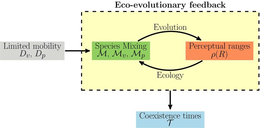
large area [25–27], whilst also allows for the presence of prey crowding effects [28, 29].
                    These trade-offs bound the evolution of the perception range, setting a finite optimal
                    value. Overall, due to its large intraspecific variability, important contribution to
                    individual fitness and sensitivity to species spatial distribution, the perceptual range
                    arises as an important trait for studying the interplay between its evolutionary
                    dynamics and spatial ecological processes within the community.
                        In fact, our results reveal the existence of a feedback between the evolution of the
                    predator perceptual range and species spatial distributions that controls
                    community-level processes. We perform a systematic investigation of the
                    predator-prey dynamics under different levels of mobility and mutation intensities and
                    characterize the community long-time behavior by species mixing measures, by the
                    distribution of predators’ perceptual range and by species coexistence time period.
                    Depending on individual mobility (and the interactions taking place), different levels
                    of spatial mixing emerge, ranging from segregation to high mixing, and select for
                    different perceptual ranges. Simultaneously, due to predation, perceptual ranges alter
                    the spatial mixing of preys and predators, establishing an eco-evolutionary feedback.
                    Importantly, since species mixing modulates the intensity of the prey-predator
                    interaction, the eco-evolutionary feedback strongly influences the stability of the
                    community. A diagram with the coupling between species spatial distribution,
                    individual traits and community level processes is shown in Fig 1. Finally, although
                    derived for the particular case of a prey-predator system, these results will more
                    generally improve our understanding of how information gathering over nonlocal
                    spatial scales may influence species interactions and how evolutionary processes may
                    alter the ecological dynamics and stability of spatially-structured multispecies
                    communities.

                    Results
                    To investigate the interplay between spatial structure and evolution of the range of
                    nonlocal interspecific interactions in a simple community (see the diagram shown in
                    Fig 1) we build an individual-based prey-predator model (see Methods for full details)
                    in which individuals of both species move within a square environment of lateral
                    length L (and periodic boundary conditions). Movement is modeled using Brownian
                    motions with diffusion coefficients Dp for predators and Dv for preys (v stands for
                    victims), which influences the spatial distribution of the populations (Fig 2). Large
                    diffusion leads to homogeneously distributed populations, whereas clusters form at low
                    diffusion due to the existence of reproductive pair correlations [30].
                        We implement a stochastic population dynamics in which prey reproduction and
                    predator death occur with constant rates r and d, respectively. The predation rate, c,
                    however, is dictated by the availability of preys and the efficiency of the predator to
                    attack them. Mathematically, this can be written as c(R) = E(R)Mv (R), where
                    Mv (R) accounts for the number of preys within predator’s perceptual range, R, and
                    E(R) is the attacking efficiency up to distance R. We have defined the perceptual
                    range R, different for each predator, as the maximum distance measured from the
                    position of the predator at which a prey can be detected. Note that 0 ≤ R ≤ L/2, due
                    to the periodic boundary conditions. If the perception range is large, the number of
                    available preys increases, but it does so at the cost of a reduced predation likelihood.
                    We implement this trade-off through the attacking efficiency E(R), which we assume
                    to be a decreasing function of the predation range. The particular shape of E(R) may
                    depend on several factors, related to prey, predator behavior or environmental features.
                    To be specific, we assume that the attacking efficiency decays exponentially with the
                    perception range as E(R) = c0 exp(−R/Rc ), where c0 is a maximal efficiency and Rc

February 11, 2019                                                                                        3/22
Fig 1. Schematic representation of the eco-evolutionary framework. In the
gray box the microscopic parameters Dv and Dp are the prey and predator diffusion
coefficients that set the level of mobility. The rest of the elements are properties at the
community level that arise from them and from the demographic rates. In the green
box species spatial distribution characterization though the mixing measures M, Mp ,
Mv . In the orange box predators perceptual range distribution ρ(R). In the blue box,
community coexistence times T . Arrows indicate the influence between the elements
through different processes.
fixes how quickly this efficiency decays as the perception range increases. For this
particular choice, and considering a homogeneous distribution of preys, Mv (R) ∝ πR2 ,
the predation rate c(R) ∝ R2 exp(−R/Rc ) is thus maximized for Rh⋆ ≡ 2Rc . We will
use this value Rh⋆ as a reference to measure the effect of mutations and
nonhomogeneous distributions of individuals on the optimal perception range.
The trade-off between perception and attacking efficiency, as well as the choice of
E such that predation rate maximizes at intermediate scales of perception, is
grounded on previous theoretical studies showing that foraging success decreases when
individuals have to integrate information over very large spatial scales [25–27, 31].
Another example that can illustrate the trade-off between perception and predation
efficiency is that of flying predators, whose flight altitude influences the area where
preys can be detected. However, even though flying at high altitudes opens the field of
view and possibly the number and frequency of prey detection it may also have a
negative effect on predation success, since attacks are initiated from further away.
Note that we do not model the attack process, that we consider to be instantaneous.
Thus, the predator mobility described by the diffusion coefficient Dp refers to the
predator motion while searching.
Ultimately, prey consumption will support predator reproduction. To model this,
whenever a prey is caught by a predator, there is a probability b for the predator to
reproduce. Hence, predators reproduction rates are determined by the interplay
between their perception range and the spatial configuration of preys. Ignoring any
complex phenotype-genotype relationship and the role of the environment [32], we
assume that newborns inherit the perceptual range from their parent, with some
possible mutation that adds to R a random perturbation sampled from a Gaussian of
zero mean and variance σµ2 . This trait remains unchanged during predators’ lifetime.
The mutation intensity σµ sets the speed of the evolutionary process. Mathematical
details of the model and its implementation are provided in Methods.
Since we are interested in how the coupling between limited dispersal and evolution
in the perception ranges influences the stability of the community, we fix all the model
February 11, 2019 4/22Fig 2. Species spatial distribution. Spatial distribution of predators (red) and
preys (blue) in the long-time regime for (A) low and (B) high mobility, with
Dp = Dv = 0.1 and Dp = Dv = 1, respectively. Gray circles indicate the perception
area of the predators, which is subject to evolutionary dynamics (with σµ = 0.1, see
Methods for details). The habitat is a square domain with size L = 20 and periodic
boundary conditions. See S1 Movie and S2 Movie to visualize the model dynamics.
parameters (see Methods) except the intensity of the mutations in R, σµ , and the
diffusion coefficients Dv and Dp , which are the control parameters that drive the
degree of mixing in the population (for computational convenience, different values of
L will also be used). Therefore, for a given pair of diffusion rates and a mutation
intensity, three linked community-level features emerge: the species spatial
distributions, the distribution of predator perceptual ranges (i.e., the outcome of the
evolutionary dynamics) and the coexistence time of the populations. In the following
sections we examine each of these features more in depth.
Species spatial distributions
For fixed prey birth and predator death rates, the spatial distribution of preys and
predators is determined by three characteristic spatial scales, controlled by Dv , Dp
and R. Fig 2 shows that for large diffusivities (right panel) both predators and preys
are homogeneously distributed, whereas they form clusters for low diffusion
coefficients (left panel).
In order to quantify population clustering within each species, as well as
interspecies mixing, we define the indicators Mv and Mp for the former and M for
the latter. These quantities are defined in terms of the Shannon index or
entropy [33–35], conveniently modified to correct for the effect of fluctuations in the
number of individuals (see Methods for the mathematical definitions). The
interspecies mixing M takes values between 0 and 1, with 0 indicating strong species
segregation and 1 representing the well-mixed limit. On the other hand, Mp and Mv
also take values within the same range, but since these metrics focus on one single
species, Mα = 0 indicates a high level of clumping of species α (= v or p) and Mα = 1
a uniform distribution of the corresponding species.
The mixing measures are sensitive to the diffusion coefficients and predators
perception range. First, we analyze the spatial distribution of species at a fixed
February 11, 2019 5/22mutation intensity and in the long-time limit, i.e., once the distribution of perceptual
ranges reached a stationary form.
For a fixed mutation-noise standard deviation (σµ = 0.1), Fig 3 shows the average
values of the mixing measures in the long-time regime as a function of the individuals
mobility, revealing a complex interaction between mobility and species mixing. When
both preys and predators have the same diffusion coefficients, Dv = Dp , all the mixing
indices increase with mobility (Fig 3A). However, when species have different diffusion
coefficients, Dv 6= Dp , the mixing may become a non-monotonic function of one of the
diffusion coefficients. For the particular case shown in Fig 3B, the prey mixing still
increases monotonically with Dv , but the interspecies and the predator mixing show a
maximum at intermediate Dv . Prey population can be seen as a dynamical resource
landscape that drives the spatial distribution of predators. Increasing Dv always leads
to a more uniform distribution of preys. However, the extent to which this also leads
to more uniform distributions of predators is limited by Dp (which in Fig 3B is fixed
at a low value Dp = 0.1). In particular when Dv ≫ Dp predators cannot follow the
dynamics of the preys and both M and Mp decrease with increasing Dv .
Fig 3. Species mixing. Average predator-prey mixing hMi and prey and predator
mixing, hMv i, hMp i, respectively, for different individuals mobility with (A) Dp = Dv
and (B) Dp = 0.1. Mutation intensity is σµ = 0.1 and habitat size L = 10. Average is
performed over time and 104 realizations in the long-time regime.
Next, we explore the effect of the mutation intensity on the long-time average
interspecies mixing, hMi (angle brackets indicate average over time and realizations).
In the non-evolving case, i.e. in the no-mutation limit (σµ = 0) and setting the same
perceptual range R for all predators, mixing is a convex function of R, showing a
minimum for intermediate perception ranges (see S1 Fig). The values of R giving
minimum mixing without evolution (S1 Fig) are close to the ones dynamically
achieved under evolution (see section Evolutionary dynamics), stressing the fact that
predation reduce interspecies mixing. When mutations are allowed (σµ > 0), however,
predators’ perceptual range are not free parameters, but an outcome of the
eco-evolutionary dynamics and thus controlled by the individuals mobility and
mutation intensity. In particular, in Fig 4, fixing Dv = Dp , we show how σµ changes
the predator-prey mixing curve shown in Fig 3A. To this aim we define the relative
change with respect to the no-mutation limit case (σµ = 0), in which all predators
February 11, 2019 6/22have the optimal perceptual range R⋆ (see section Evolutionary dynamics),
hMi(Dv , Dp |σµ ) − hMi(Dv , Dp |σµ = 0)
∆hMi(Dv , Dp |σµ ) ≡ , (1)
hMi(Dv , Dp |σµ = 0)
where brackets indicate average over time and realizations in the long-time regime.
Fig 4. Mixing dependency on mutation intensity. Average predator-prey
mixing change relative to the no-mutation case, ∆hMi defined in Eq (1), as a function
of the diffusion coefficients Dv = Dp and for different levels of mutation noise variance.
Habitat size L = 10. Symbols indicate the results from simulations. Dashed lines are
smooth fits to simulation data for different mutation intensities. The horizontal
continuous line ∆hMi = 0 is the no-mutation case (σµ = 0). Vertical line indicates the
maximum mixing for σµ = 1.0.
While at low mobility interspecies mixing is reduced as mutation noise σµ increases
(i.e. more segregated predator-prey distributions will be obtained for larger mutation
intensity), at high mobility the effect is the opposite. Particularly, at intermediate
mobility, the mixing suffers a maximum positive change. These effects arise mainly
from the mutation-induced variability in the values of R in the predator population,
which will be discussed in the next section.
Evolutionary dynamics
In our model we assume that predators perceptual range (and thus predator
reproduction rates) are subject to natural selection. We neglect any complexity in the
genotype-phenotype relationship and the role of environment [32], assuming that the
value of the trait R of a predator is passed to its offspring, with some variation due to
mutation, remaining unchanged during its lifetime. Natural selection is at work since,
depending on the spatial distribution of preys, some perceptual ranges are favored
against the others and hence tend to be overrepresented within the populations.
Homogeneous limit. In the Dv , Dp → ∞ limit (which leads to
M, Mv , Mp → 1), the populations of preys and predators are randomly distributed in
February 11, 2019 7/22space and well-mixed with each other. In this homogeneous mean-field limit, it is
possible to derive an equation for the dynamics of the distribution of perceptual
ranges in the population, ρ(R). We define its normalization
R such that its integral
gives, at each time, the total number of predators, Np : dRρ(R) = Np . On average,
and in the absence of any mutation effect, the encounters between preys and predators
] given by
lead to an expected rate of change of ρ(R), ρ(R),
] = bρ(R)hc(R)ip ,
ρ(R) (2)
which is proportional to the mean predation rate hc(R)ip (averaged over all predators
that experience different environments but with the same R) multiplied by the
probability b of birth after a predation event. In this homogeneous limit, and if the
number of individuals is large enough so that we can neglect demographic fluctuations,
the expected number of preys within a radius R is hMv (R)ip = πR2 v. v is the
(uniform) density of preys. Thus hc(R)ip = hE(R)Mv (R)ip = c0 πR2 ve−R/Rc (see
Methods for further details). Next, considering the effect of mutations, which changes
the perception ranges of the new individuals, and adding the contribution from the
predator death at fixed rate d, the distribution of perception ranges evolves according
to
Z L/2
∂ρ(R, t)
= Gµ (R, R′ )^
ρ(R′ )dR′ − dρ(R)
∂t 0
Z L/2
′
= πbc0 v Gµ (R, R′ )ρ(R′ )(R′ )2 e−R /Rc dR′ − dρ(R) , (3)
0
while prey-density changes follow
L/2
dv
Z
= rv − hc(R)ip ρ(R)dR ,
dt 0
Z L/2
= rv − πc0 v R2 e−R/Rc ρ(R)dR , (4)
0
where the first term represents prey birth at constant rate r and the second one
accounts for predation.
The integral kernel Gµ relates newborn with parental perceptual ranges and thus
depends on mutations. Recall that these mutations are random perturbations that
follow a Gaussian distribution of zero mean and variance σµ . The kernel Gµ should
also account for boundary conditions in R, such that mutations leading to perception
ranges that would be negative or larger than half of the system size are rejected. Thus,
Gµ is a Gaussian function restricted to the interval [0, L/2],
−(R−R′ )2
2
1
′
Gµ (R, R ) = N (R) e 2σµ
0 < R′ < L/2 , (5)
0 else
where N is a normalization factorgiven by
pπ h R R−L/2
i
N (R) = 2 σµ erf √
2σ
− erf √
2σ
. The agreement between the theoretical
µ µ
prediction for the well-mixed case (Dv , Dp → ∞), computed from Eqs (3)-(5), and
direct simulations of the individual-based dynamics is shown in Fig 5. The
infinite-diffusion homogeneous limit is implemented in the simulation by randomly
redistributing predators and preys in space at each time step. Starting from any initial
distribution, the maximum of the time-dependent distribution ρ(R), that defines the
dominant perceptual range R⋆ , approaches values near the one that gives the
February 11, 2019 8/22maximum catching rate Rh⋆ = 2Rc (Fig 5A). The long-time dominant value
corresponds exactly to the optimal one, Rh⋆ , when mutation is negligible. As mutation
intensity σµ increases, the long-time distribution ρ(R) becomes wider and there is also
a small shift towards larger values (Fig 5B), which arises due to the asymmetric form
of the catching rate hc(R)ip . Thus, the dominant R has a main component set by the
optimal value and a small positive shift due to mutation effects. These changes,
specially the strong effect observed in the perceptual range variability, are the ones
responsible for the feedback in the predator-prey mixing shown in Fig 4. The
corresponding result from individual-based simulations is obtained by averaging over
independent runs the perceptual range distribution ρ(R) at each time, and extracting
its maximum R⋆ at that time. The agreement between both results persists as long as
the number of individuals is large. Lastly, note that Eqs (3)-(4), recover the classical
Lotka-Volterra predator-prey equations in the limit of vanishing trait variability,
ρ(R, t) → Np δ(R − R⋆ ).
Fig 5. Evolutionary dynamics in the homogeneous limit. (A) Temporal
evolution of the dominant perception range R∗ (the mode, i.e. the maximum of ρ(R)),
relative to the one giving the maximum predator growth in the homogeneous case, Rh∗ ,
for σµ = 0.1 and a system size L = 40. Solid line is obtained from numerical solution
of Eqs (3)-(4), and dots give the maximum of the distribution ρ(R) obtained from the
average of 100 independent runs of the individual-based model with Dv , Dp → ∞. In
all cases the initial distribution gives weight only to R = 2Rh⋆ . (B) Probability density
for finding a perception range value R in the population of predators, ρ̄(R) = ρ(R)/Np ,
in the long-time regime, for low and high mutation noises. Dots correspond to
simulations of the individual-based model (with Dv , Dp → ∞, average over 100 runs)
and solid lines to the numerical solution of Eqs (3)-(4). Dashed vertical lines show the
position of the mode of each distribution.
Finite mixing case. For the general case of limited dispersal, far from the
well-mixed scenario, some of the features shown in Fig 5 still persist, but modified due
to the underlying spatial distribution of preys and predators. Since the analytical
approximations derived for the infinite diffusion limit are not valid, we study this
scenario via numerical simulations of the individual-based model. In Fig 6A we show
that, starting from different initial distributions of R, the location R∗ of the maximum
of the average distribution ρ(R), giving the most probable value of R, evolves in time
towards a value that depends on the mobility of both species, with reduced mobility
February 11, 2019 9/22favoring larger perceptual ranges (Fig 6B). The change in ρ(R), both with time and
with species mobility in the long-time limit, is shown in S2 Fig. The most probable
perception range decreases with increasing predator and prey diffusion rates, and it
approaches the homogeneous value as a power-law (see inset of Fig 6B).
Fig 6. Dominant perceptual range: from the segregated to the well-mixed
scenario. (A) Temporal evolution of the location R⋆ of the maximum in the average
perception range distribution ρ(R) (average over 104 runs), relative to the optimal
perception range for homogeneous populations, Rh⋆ , for high (Dv = Dp = 1.0) and low
(Dv = Dp = 0.1) diffusion coefficients. Two different sharply-localized initial
population distributions are used in each case. Bars indicate the standard deviation of
ρ(R) around R⋆ . (B) Dominant perception range relative to the homogeneous-case
optimal, R⋆ /Rh⋆ , as a function of prey and predator diffusion rates. Dashed lines are
guides to the eye and indicate the discretization ∆R = 0.1 used for the numerically
obtained ρ̄. Inset shows the asymptotic approach of R⋆ to the homogeneous optimal,
Rh∗ , as Dv increases with Dp = 0.1. (C) The relative difference between the dominant
range in the simulations and the optimal one in the homogeneous case, |R⋆ − Rh⋆ |/Rh⋆
versus 1 − hMv i, which measures prey clumping (averaged over time and realizations
in the long-time regime), for different values of prey diffusion Dv , while keeping
Dp = Dv (circles) or Dp = 0.1 (squares). Bars indicate bin size of the computationally
obtained ρ(R). Dashed lines represent the power-law expressions set in Eq. (6), with
γ ≃ 1.5 for Dp = Dv and γ ≃ 0.5 for Dp = 0.1. Habitat lateral length L = 10 and
mutation intensity σµ = 0.1 in all the panels.
We identify that the change in the dominant perception range due to mobility is
well captured by the prey mixing parameter Mv : Fig 6C shows the dominant R in the
long-time regime as a function of prey clumping. We extract that
|R⋆ − Rh⋆ |
= (1 − hMv i)γ , (6)
Rh⋆
with γ ≃ 1.5 (γ ≃ 0.5) when fixing Dp = Dv (Dp = 0.1) and mutation intensity
σµ = 0.1. This relation is valid for low mutation intensity, such that in the well-mixed
scenario, Mv → 1 (achieved for large diffusivities), we have R⋆ ≃ Rh⋆ . The prey
mixing is the main quantity that controls the dominant perceptual range as it
condense the spatial information of the environment experienced by predators. As
prey form clusters, Mv < 1, predators typically find preys at distances larger than in
the homogeneous case (see Fig 2). So, in the low-mobility regime their predation rate
only becomes significant for larger R.
February 11, 2019 10/22Coexistence times and extinction probabilities
We have observed in the previous sections that the eco-evolutionary feedback between
evolution of perception ranges and species mixing controls predation rates. Thus, we
expect it to impact also the population dynamics and the stability of the community.
To quantify this, we measure the coexistence time between preys and predators, T ,
and the probability that preys get extinct before the predators, β, as a function of the
predator and prey mobilities and the intensity of the mutations. Mean coexistence
time T is defined as the time until either preys or predators get extinct, averaged over
independent model realizations, and β is obtained as the fraction of realizations in
which predators persist longer than preys. Since preys are the only resource for
predators, these will shortly get extinct following prey extinctions. On the contrary,
when predator extinctions occur first, preys grow without constraint because we do
not account for interspecific competition. For each realization we use initial conditions
that lead to a very short transient after which spatial structure and the perceptual
range distribution achieve its long-time behavior. In most cases, the well-mixed mixed
scenario with uniformly distributed perceptual range allow this to happen.
Nevertheless, for small mutation rates (σµ < 0.1), the evolutionary time scales become
comparable to the coexistence times and in these cases we need to fast forward the
evolutionary component of the transient dynamics by setting an initial condition for
the perceptual range distribution close to the expected at long times.
In Fig 7A we show the mean coexistence time T as a function of predator and prey
diffusion coefficients, assuming Dv = Dp , for different mutation intensities. This curve
is a complex outcome of the values of the dominant perceptual range, the associated
catching rate, and the degree of mixing that arise from limited dispersal. Long
coexistence would occur when there is a balanced mixing between preys and predators,
which allows predation in a controlled manner, preserving prey population. For small
mutation intensity, the coexistence time, which is maximum at low diffusivities,
decreases as the diffusion coefficients increase until reaching a minimum at
intermediate mobility. Then, T increases slowly, approaching asymptotically the
well-mixed case. As mutation increases there is a clear change in the depependence of
T with the diffusivities. The maximum of T is shifted to intermediate values of
diffusivities. This is one of the relevant results of this paper. This result comes from
the effect that mutation intensity (when non-negligible) has in predator-prey mixing,
as shown in Fig 4: mixing decreases for low mobility and increases at intermediate
values of the mobility. Since mixing controls interspecies interaction, a key ingredient
for coexistence, this is translated to the behavior of T . As seen in Fig 7A, the level of
mobility at which the increase in mixing is maximum (vertical dashed line, from Fig
4) roughly matches the location of the maximum T .
As discussed in the previous sections, mutation intensity interferes in predator-prey
mixing mainly through its influence in perceptual range variability (see Fig 5B),
establishing the feedback that mediates community coexistence. Despite that,
variability in R brings secondary effects. For instance, variability gives resilience to
the community, since it allows predators to overcome time periods in which, due to
fluctuations in the spatial distribution of preys, the (on average) optimal R is
temporarily suboptimal. Also, variability reduces overall predators’ predation success.
Finally, we calculate the probability that preys become extinct before predators β,
as a function of Dv (which is taken to be equal to Dp ) for different values of σµ
(Fig 7B). Even though the most likely event is that predators disappear before preys
(β < 0.5), as the diffusion coefficients increase from very small values, we observe an
increase on β passing through a maximum at intermediate values of diffusivities.
Despite the nonlinear effects between catching rate and species spatial distributions, β
generally becomes large as mixing increases (see Fig 3A and Fig 7B), since it enhances
February 11, 2019 11/22Fig 7. Community coexistence times and prey extinction probability. (A)
Mean coexistence time T and (B) Probability of prey extinction before predators, β,
as function of the diffusion coefficients Dp = Dv for different levels of mutation noise
intensities with system size L = 10. Initial conditions are preys and predator
uniformly distributed in space with uniformly distributed perception range R, and
results were extracted from 5 × 10³ realizations. Dashed lines are smooth fits to guide
the eyes. Vertical dashed lines indicate the diffusivity value at which the increase of
mixing with respect the no-mutation case is maximum (from Fig 4, σµ = 1.0)
predation. Note that, comparing Figs 7A and 7B, the maximum β (high predation) is
not related to maximum coexistence, which calls for an ideal balance between catching
and prey population preservation. The influence of mutation intensity in the profiles
shown in Fig. 7B, again, is due to the feedback in the interspecies mixing shown in
Fig 1, which regulates the level of predation. Hence, prey extinction is reduced at low
mobility but increased at high mobility, shifting the profile.
Summary and Discussion
Using an individual-based model, we have investigated whether the evolutionary
dynamics of predator perceptual ranges influences the stability of spatially-structured
prey-predator communities. First, we studied how different levels of interspecies
mixing arise due to limited mobility and variability in the perceptual range induced by
the intensity of mutations. Second, we evaluated the consequences of the interplay
between species mixing and the predator perception range in other community-level
outcomes. Our results reveal the existence of an eco-evolutionary feedback between
February 11, 2019 12/22interspecies mixing and predators perception: species mixing selects a certain
distribution of perceptual ranges due to an underlying perception-vs-attacking
efficiency trade-off; in turn, the distribution of perceptual ranges reshapes species
spatial distribution due to predation. More specifically, when species mobilities are
low, preys and predators form monospecific clusters and thus segregate from each
other. Therefore, preys often inhabit regions of the environment that are not visited
by predators, which forces the evolution of larger predatory perception. Conversely, as
mobility becomes higher, species mixing increases and short-range predation is favored.
Finally, our results indicate that community stability and diversity, characterized by
the mean coexistence time and prey extinction probability, are strongly controlled by
the eco-evolutionary feedback. In particular, the average coexistence time is maximum
when the interaction between species mixing and predator perception ranges yields in
predation rate that is large enough to sustain the population of predators but low
enough to avoid fast extinctions of preys.
The two community-level metrics, mean coexistence time and species extinction
probabilities, provide important information about the diversity of the community at
different scales [36]. From a metapopulation perspective, each model realization
performed to obtain these observables can be related to the dynamics taking place
within distinct local regions, known as patches. In our case, since realizations are
independent, these patches are isolated (not coupled by dispersal events) and
constitute a “non-equlibrium metapopulation” [37]. In this context, the mean
coexistence time is a proxy for alpha (intra-patch) diversity, i.e. how long species
coexist in each patch, whereas species extinction probabilities inform about the beta
(inter-patch) diversity, i.e., how many patches are expected to be occupied by preys
and how many by predators once one of the species has been eliminated. Using a
mathematical reasoning, the fractionR ∞ of patches in Rwhich predators and preys coexist
t
at any time t is given by P (t) = t p(t′ )dt′ = 1 − 0 p(t′ )dt′ , where p(t) is the
distribution of coexistence times. Supported by our numerical simulations, we can
approximate p(t) ≃ T −1 e−t/T (except for coexistence times that are much smaller
than the mean, see S3 Fig). Therefore, P (t) ≃ 1 − e−t/T . The fraction of patches
occupied only by preys is given by (1 − β)(1 − P (t)), and the fraction of patches in
which overexploitation has caused prey extinction is given by β(1 − P (t)). Hence, the
mean coexistence time T and the prey extinction probability β quantify the diversity
of the community at different spatiotemporal scales [33, 36, 38], that might serve as
important guides for the design of ecosystem management protocols [38, 39].
Since we were interested in studying whether the spatial coupling between mobility
and perception could lead to an eco-evolutionary feedback when both processes occur
at comparable time scales [14, 15], we kept all the characteristic time scales of the
system fixed, except those related to diffusion and the evolutionary dynamics of
perceptual ranges. In this scenario, provided that evolution is fast enough, the spatial
distribution and the distribution of perceptual ranges relax to their stationary values
in timescales much shorter than the characteristic time scales at which
community-level processes occur, defined by the mean coexistence time. Under this
condition, the long-time regime is well-defined and can be characterized by constant
quantities. A sensitivity analysis on reproduction rates and initial conditions reveals
that, as far as this relationship between time scales is maintained, both the existence
of the eco-evolutionary feedback and its impact on community stability and diversity
remain unaffected. This condition can be broken, for instance, if predator and prey
birth-death rates are small, or too unbalanced, producing very short coexistence times.
Our results are also robust against changes in the source of individual-level trait
variability, as individual-level trait variability affect mixing in a similar way. In this
work, we have considered the case in which variability is induced by mutation in the
February 11, 2019 13/22transmission of the trait, but variability can be rooted in non-inheritable properties,
such as body size or the individual internal state (level of hunger, attention...) [25],
that do not introduce spatial correlations between trait values. We have seen that
sampling predators’ newborn perceptual range from a suitable fixed distribution
(being independent on the parents’ trait), we are able to mimic the results shown in
Fig. 7. This implies that different processes that promote variability can control
community coexistence.
Finally, although we have focused here on a prey-predator dynamics, our results
will more generally illuminate whether and to which extent the interplay between
species spatial distributions and evolution shaping the range of ecological interactions
and information gathering processing may determine several community-level
outcomes, such as diversity, stability and the distribution of traits. Therefore, our
study opens a broad range of questions and directions for future research. First, we
have limited to the case in which only predator traits can evolve, whereas evolution of
prey traits has been also shown to impact profoundly the population dynamics of both
species in well-mixed settings [21]. A natural extension of our study would be to
explore such scenario in a spatially-extended framework as the one introduced here.
More complex possibilities, such as the co-evolution of traits in both species could also
shed some light on the possible existence of new population dynamics [19] or more
general evolutionary processes, such as arm races in phenotype space (red queen-like
dynamics) instead of trait distributions reaching a stationary configuration [40].
Different movement models, such as Lévy flights instead of Brownian motion, can
modify both the optimal range of the interactions [27] and the emergence of clusters of
interacting individuals [41], possibly leading to new community-level results. The
existence of environmental features that could also affect the degree of mixing and its
coupling with the range of interactions, such as the presence of external flows, would
extend our results to a wider range of ecosystems in which the importance of rapid
evolutionary processes has been already reported [42, 43].
Methods
Model details
The model mimics the eco-evolutionary dynamics of a prey-predator system in a
square environment of lateral length L. Each predator and prey has a position in
space. In addition, each predator has a different perceptual range R that determines
Rthe distribution, in the population of Np predators, of this trait (ρ(R), with
dRρ(R) = Np ). Three ingredients conform the dynamics of this individual-based
model: population dynamics, evolution with mutation, and individual dispersal.
1. Population dynamics. The number of preys, Nv , and predators, Np , change in
time due to prey reproduction, predator death and predation. These processes
are modeled as Poisson processes that occur at rates that may depend on the
different densities and perceptual ranges. Each predator may die at a constant
rate d and may catch a prey with rate c(R) that depends on its perceptual range.
If a certain predator catches a prey, it reproduces with probability b, generating
at its position a new individual which inherits its trait R, possibly modified by a
mutation. Preys, on the other hand, reproduce with constant rate r and die as a
consequence of predation events. These processes can be written in the form of a
February 11, 2019 14/22set of biological reactions for preys V and predators P
r
V −
→V +V ,
d
P −
→ ∅, (7)
(
c(R) P + P̃ with probability b
P + V −−−→
P with probability 1 − b ,
where we added the notation P̃ to indicate that the predator newborn might
have its trait slightly modified from the parental value due to mutation (see
Eq (10) below).
Each predator detects preys within a disk of radius given by its perceptual range
R, with every prey inside that region equally likely to be caught. Following
previous results that link the perceptual ranges, information gathering and
foraging success [25–27, 31], the model accounts for a trade-off between
perceptual range and predation efficiency E(R), such that while large perceptual
range increases the potential number of preys, predation efficiency decreases.
Combining these effects, for a given predator the predation rate can be written as
c(R) = E(R)Mv (R) , (8)
where Mv (R) is the number of preys within the predation disk of radius R
centered at the position of each predator. Since Mv (R) is a monotonically
growing function of R, the shape of E determines whether the predation rate
maximizes at a certain perceptual range. The efficiency function E is expected
to introduce an upper bound to viable perceptual ranges. This conditions is
fulfilled if, for large R, the efficiency decays faster than the increasing number of
preys in the range, Mv (R). In the case of homogeneously distributed particles,
Mv (R) ∝ R2 . In this case, the catching rate c has a nontrivial maximum at a
finite value of R if E decays faster than R−2 . To be specific, an exponential
decay is assumed for the attacking efficiency,
E(R) = c0 e−R/Rc , (9)
where Rc sets the distance at which E significantly decays and c0 is proportional
factor. For the spatially homogeneous case, we find that c(R) ∝ R2 exp(−R/Rc ),
which has a maximum at Rh⋆ ≡ 2Rc . This optimal value Rh⋆ is used as a reference
in our results.
2. Evolution with mutation. Each predation event is followed by the possible
reproduction of the predator, occurring with probability b. In this case, besides
inheriting the parental position, the newborn individual also inherits the
parental perceptual range, R, but with an added random perturbation, ξµ , which
models mutations and thus giving rise to a modified value of the trait R̃,
R̃ = R + ξµ . (10)
ξµ is a zero-mean Gaussian variable whose variance, σµ2 , regulates the intensity of
the mutations. In order to avoid perceptual ranges that exceed system size or are
negative, mutations leading to R < 0 or R > L/2 are rejected. We neglect any
complexity in the genotype-phenotype map, so that we consider the phenotypic
trait R to be directly determined by the parental one and the mutations.
3. Individual dispersal. Individuals are assumed to follow independent
two-dimensional Brownian motions with diffusion constants Dv and Dp for preys
February 11, 2019 15/22and predators respectively. The position of every individual is updated after
each time step ∆t (to be defined by the Gillespie algorithm described below) by
sampling a turning angle, θ, and a displacement, ℓ. The turning angle follows a
uniform distribution between [0, 2π), and the traveled distance is obtained from
the absolute value of a normal random variable with zero mean and variance
proportional to the individual’s diffusion coefficients. Periodic boundary
conditions are implemented. Mathematically, this position updating for
individual i can be written as
xi → xi + ℓθ̂ ∀ i ∈ {1, 2, . . . , Np + Nv } , (11)
where θ̂ is a random direction and ℓ the length of the
√ displacement of the jump,
sampled from p(ℓ > 0) ∝ exp[−ℓ2 /(2ℓ̄2 )], being ℓ̄ = 2Di ∆t with Di = Dv , Dp
the individual’s diffusion coefficient and ∆t the simulation time step as will be
detailed below.
Model implementation: the Gillespie algorithm
We implement the stochastic birth-death dynamics, occurring at Poisson times
depending on the respective rates, following the Gillespie algorithm [44–46]: First,
from a configuration with Np predators and Nv preys, the predation rate c(Ri ) is
computed for each predator, of perceptual range Ri . Next, recalling that predator
death (d) and prey reproduction (r) rates are the same for all individuals, the total
PNp
event rate is computed [44] as g = rNv + i=1 [c(Ri ) + d]. Then, we compute the
time-step ∆t to the next demographic event as ∆t = ζτ where ζ is an exponentially
distributed random variable with unit mean and τ ≡ 1/g, the average time to the next
event. After this ∆t, a single event will occur, prey reproduction, predation or
predator death, chosen from all the possible events (and individual involved) with
probability proportional to the contribution of the respective rate (see Eq (7) and (8))
to the total rate g. If predator death or prey reproduction occur, we simply remove or
generate a new individual at parents’ position, respectively. If predation occurs, a prey
randomly chosen within the perception range of the selected predator dies and, with
probability b, a new predator is generated at the same location as the predator, with
value of the perception range obtained from Eq (10).
For simplicity, we fix in this paper the values r = d = c0 = b = Rc = 1 and focus
our study in the influence of the different values of diffusion coefficients Dp and Dp ,
and mutation rate (for computational convenience we use also different values of
system size L). The impact of changing the rates to other values is briefly addressed
in section Summary and Discussion.
Mixing measures
In order to quantify the spatial arrangement of the species, we define measures of
mixing. A possible way to proceed is to use the Shannon index or entropy, which has
been applied to measure species diversity, racial, social or economic segregation on
human population and as a clustering measure [33–35]. Based on these previous
approaches, we propose a modification described below.
As usual,
√ we start regularly partitioning the system in m square boxes with size
δx = L/ m and obtaining for each box i the entropy index si [34], given by
si = −fp(i) ln fp(i) − fv(i) ln fv(i) , (12)
(i) (i)
where fp (fv ) is the fraction of predators (preys) inside box i, i.e.
(i) (i) (i) (i) (i) (i)
fq = Nq /[Np + Nv ] with q = p, n and Np , Nv the numbers of predators and
February 11, 2019 16/22preys in that box, respectively. In terms of Eq (12), predator-prey mixing is maximum
when there is half of each type in the box, yielding si = − ln 1/2 = ln 2. Unbalancing
the proportions of the two types in the box reduces si . If a box contains only
predators or preys, si = 0, indicating perfect segregation. Finally, we define a
whole-system predator-prey mixing measure by averaging the values si in the different
boxes, each one weighted by its local population [34],
m
X N (i)
hMim ≡ si , (13)
i=1
N
(i) (i)
being N (i) = Np + Nv the total box population and N = Nv + Np the total
population. To really characterize the lack of inhomogeneity arising from interactions
and mobility, one should compare the value of hMim with the value M that would be
obtained by randomly locating the same numbers of predators and preys, Np and Nv
among the different boxes. At this point, approximations for M which are only
appropriate if the number of individuals is large have been typically used. In our case,
since predator and prey populations have large fluctuations, it is necessary to give a
more precise estimation. In a brute force manner, one can obtain computationally the
mixing measure for the random distribution simply by distributing randomly in the m
spatial boxes the Nv preys and Np predator and averaging the corresponding results of
Eq (13) over many runs. On the other hand, this can be done analytically since we
known that, for random spatial distribution, the number of individuals nq of type q
(= p, v) in each box would obey a binomial distribution B(nq , Nq ), where Nq is the
total particle number
1 nin the system. We have that
B(nq , Nq ) = N q q 1 Nq −nq
nq ( m ) (1 − m ) . Then, Eq (13) for randomly mixed individuals
becomes
Nv XNp
X nv + np
M≡ B(nv , Nv )B(np , Np ) s(nv , np ) , (14)
n =0 n =0
Nv + Np
v p
with s as defined in Eq (12).
Finally, a suitable measure of predator-prey mixing that characterizes spatial
structure from the well-mixed case (M = 1) to full segregation (M = 0) is given by
hMim
M≡ . (15)
M
Also, we can define an analogous measure for each species’ spatial distribution
separately, which can be interpreted as a degree of clustering [35],
m (i) (i)
1 X (Nv /Nv ) ln(Nv /Nv )
Mv = − , (16)
Mv i m
and
m (i) (i)
1 X (Np /Np ) ln(Np /Np )
Mp = − , (17)
Mp i m
for preys and predators respectively, where
Nv Np
X X
Mv = B(nv , Nv )[(nv /Nv ) ln(nv /Nv )] , Mp = B(np , Np )[(np /Np ) ln(np /Np )] .
nv =0 np =0
(18)
For Mv or Mp = 1, the corresponding species is well spread around the domain.
Smaller values indicate clustering of the individuals.
February 11, 2019 17/22The mixing measures are certainly affected by the size of the box δx used, which
should be tuned to obtain maximum sensibility to the spatial distribution. For very
large or very small box size, we see that different spatial distributions become
indistinguishable. For instance, for the predator-prey mixing, if the box size is very
large (of the order of system size), we will find that the predators and preys are well
mixed independent on the values of the diffusion coefficients. On the other hand, if
box size is very small it will be either occupied by a single predator or prey, if not
empty, indicating segregation independently on the individuals mobility. In S4 Fig, we
show how the mixing measure changes with box size δx and system size L for low
mobility (Dv = Dp = 0.1), which produces a highly heterogeneous spatial distribution.
We identify that for δx ≃ 2 maximum sensitivity with respect to diffusion coefficients
is attained. We used δx = 2 in our results, being a suitable scale since it is also of the
order of the typical values of the perceptual range attained under evolution.
Regarding the system size, we found only weak variations in the mixing measures,
which are shown in the inset of S4 Fig.
Supporting information
S1 Movie Temporal evolution of population spatial distribution of
predators and preys with low predator and prey mobilities. Predators and
preys in colors red and blue, respectively, Dp = Dv = 0.1, mutation noise intensity
σµ = 0.1 and habitat size L = 20.
S2 Movie Temporal evolution of population spatial distribution of
predators and preys with high predator and prey mobilities. Predators and
preys in colors red and blue, respectively, Dp = Dv = 1, mutation noise intensity
σµ = 0.1 and habitat size L = 20.
S1 Fig Mixing measures as a function of predators perceptual range R in
the non-evolving case. Predator-prey, prey and predator mixing for different values
of diffusion coefficients as a function of predators’ perceptual range R (which is fixed,
not evolving, the same for all individuals and σµ = 0). Vertical lines show the
dominant perception range achieved through the evolutionary process under low
mutation noise (σµ = 0.1). L = 10.
S2 Fig Normalized perceptual range probability density at long times and
its temporal evolution. (A) ρ̄(R) = ρ(R)/Np at long-times for low (Dp = Dv = 0.1)
and high (Dp = Dv = 1) mobility. (B) ρ̄(R) at different times (initial condition is a
sharp distribution at R = 4) obtained from the individual-level simulations for the
high mobility case Dn = Dp = 1. In both panels habitat domain has size L = 10 and
mutation intensity σµ = 0.1. The perceptual range values are scaled by the optimal
value Rh⋆ of the homogeneous case for comparison.
S3 Fig Coexistence time probability distribution. Coexistence time
probability distribution obtained from individual-level simulations with
Dv = Dp = 1, 10, 100, mutation intensity σµ = 1.0 and habitat size L = 10. Inset
shows the behavior at short timescale for the same cases. Solid red lines indicate an
exponential distribution with the same mean.
S4 Fig Mixing measures as a function of the box size used in their
calculation, and of system size. Average mixing measures for the low mobility
February 11, 2019 18/22case Dp = Dv = 0.1 for different box sizes δx. Mutation intensity σµ = 0.1 and habitat
size L = 10. Inset shows the dependence on system size L for δx = 2 (for systems sizes
in which it is not possible to set this value we take the closest points). Averages are
performed over time and realizations in the long-time regime.
Acknowledgments
We thank F. Peters for helpful discussions and IFISC (CSIC-UIB) computing lab for
technical support.
References
1. Azaele S, Suweis S, Grilli J, Volkov I, Banavar JR, Maritan A. Statistical
mechanics of ecological systems: Neutral theory and beyond. Rev Mod Phys.
2016;88:035003. doi:10.1103/RevModPhys.88.035003.
2. Ayala FJ. Competition between species: frequency dependence. Science.
1971;171(3973):820–824.
3. Chesson P. Mechanisms of Maintenance of Species Diversity. Annual Review of
Ecology and Systematics. 2000;31(1):343–366.
doi:10.1146/annurev.ecolsys.31.1.343.
4. Tarnita CE, Washburne A, Martı́nez-Garcı́a R, Sgro AE, Levin SA. Fitness
tradeoffs between spores and nonaggregating cells can explain the coexistence of
diverse genotypes in cellular slime molds. Proceedings of the National Academy
of Sciences. 2015;112(9):2776–2781. doi:10.1073/pnas.1424242112.
5. Martı́nez-Garcı́a R, Tarnita CE. Seasonality can induce coexistence of multiple
bet-hedging strategies in Dictyostelium discoideum via storage effect. Journal of
Theoretical Biology. 2017;426:104–116.
6. Tilman D. Competition and biodiversity in spatially structured habitats.
Ecology. 1994;75(1):2–16.
7. Amarasekare P. Competitive coexistence in spatially structured environments: a
synthesis. Ecology Letters. 2003;6(12):1109–1122.
8. Siepielski AM, Nemirov A, Cattivera M, Nickerson A. Experimental Evidence
for an Eco-Evolutionary Coupling between Local Adaptation and Intraspecific
Competition. The American Naturalist. 2016;187(4):447–456.
doi:10.1086/685295.
9. Kotil SE, Vetsigian K. Emergence of evolutionarily stable communities through
eco-evolutionary tunnelling. Nature Ecology and Evolution.
2018;2(10):1644–1653. doi:10.1038/s41559-018-0655-7.
10. Hiltunen T, Ayan GB, Becks L, Ayan B, Becks L. Environmental fluctuations
restrict eco-evolutionary dynamics in predator – prey system. Proceedings of
the Royal Society B. 2015;282:20150013. doi:10.1098/rspb.2015.0013.
11. Saccheri I, Hanski I. Natural selection and population dynamics. Trends in
Ecology & Evolution. 2006;21(6):341–347. doi:10.1016/j.tree.2006.03.018.
February 11, 2019 19/22You can also read