Localization in 3GPP LTE Based on One RTT and One TDOA Observation - Unpaywall

Page created by Clara Jensen
 
CONTINUE READING
Localization in 3GPP LTE Based on One RTT and One TDOA Observation - Unpaywall
Localization in 3GPP LTE Based on One RTT and
One TDOA Observation
Kamiar Radnosrati, Carsten Fritsche, Fredrik Gunnarsson, Fredrik Gustafsson and
Gustaf Hendeby

The self-archived postprint version of this journal article is available at Linköping
University Institutional Repository (DiVA):
http://urn.kb.se/resolve?urn=urn:nbn:se:liu:diva-165188

N.B.: When citing this work, cite the original publication.
Radnosrati, K., Fritsche, C., Gunnarsson, F., Gustafsson, F., Hendeby, G., (2020), Localization in
3GPP LTE Based on One RTT and One TDOA Observation, IEEE Transactions on Vehicular
Technology, 69(3), 3399-3411. https://doi.org/10.1109/TVT.2020.2968118

Original publication available at:
https://doi.org/10.1109/TVT.2020.2968118
Copyright: Institute of Electrical and Electronics Engineers (IEEE)
http://www.ieee.org/index.html
©2020 IEEE. Personal use of this material is permitted. However, permission to
reprint/republish this material for advertising or promotional purposes or for
creating new collective works for resale or redistribution to servers or lists, or to reuse
any copyrighted component of this work in other works must be obtained from the
IEEE.
1

  Localization in 3GPP LTE based on one RTT and
                one TDOA observation
          Kamiar Radnosrati, Carsten Fritsche, Fredrik Gunnarsson† , Fredrik Gustafsson, Gustaf Hendeby
                 Department of Electrical Engineering, Linköping University, Linköping, Sweden
                                       Email: {firstname.lastname}@liu.se
               † Ericsson Research, Linköping, Sweden, Email: fredrik.gunnarsson@ericsson.com

   Abstract—We study the fundamental problem of fusing one            has been extensively studied, where for instance [1]–[5] derive
round trip time (RTT) observation associated with a serving base      closed-form solutions. The hyperbolas are quadratic functions
station with one time-difference of arrival (TDOA) observation        in position, so to avoid nonlinearalities [6] transforms the
associated to the serving base station and a neighbor base station
to localize a 2-D mobile station (MS). This situation can arise in    problem into a set of linear equations and propose a method
3GPP Long Term Evolution (LTE) when the number of reported            that is suitable for real-time implementations. To increase the
cells of the mobile station is reduced to a minimum in order          reliability of TDOA positioning algorithms, [7] proposes a
to minimize the signaling costs and to support a large number         model that is applicable either if the MS is located in the
of devices. The studied problem corresponds geometrically to          near-field or far-field of the BSs. A closed-form two-step
computing the intersection of a circle with a hyperbola, both
with measurement uncertainty, which generally has two equally         non-line-of-sight (NLOS) localization technique for cellular
likely solutions. We derive an analytical representation of these     networks by means of TOA measurements is developed in [8].
two solutions that fits a filter bank framework that can keep         To deal with NLOS conditions, the authors propose a separate
track of different hypothesis until potential ambiguities have been   ranging step where an unbiased distance estimate is found. The
resolved. Further, a performance bound for the filter bank is         estimated distances are subsequently used for MS localization
derived. The proposed filter bank is first evaluated in a simulated
scenario, where the set of serving and neighbor base stations is      using trilateration. For a comparative performance analysis of
changing in a challenging way. The filter bank is then evaluated      four circular and hyperbolic geolocation methods see [9]. The
on real data from a field test, where the result shows a precision    authors in [10], use round trip time (RTT) measurements and
better than 40 m 95 % of the time.                                    report the positioning field performance in terms of availabil-
   Index Terms—CRLB, filter bank, jump Markov models, round           ity, response time, and accuracy. In [11], the MS measurement
trip time, time difference of arrival, LTE, localization              data, collected during each call/session, are shown to have
                                                                      valuable information on mobile’s performance metrics and
                                                                      also on signal strength and signal to interference plus noise
                       I. I NTRODUCTION
                                                                      ratio. The obtained information is used in a binary classifier to
   Although Global Navigation Satellite System (GNSS) sys-            infer whether the measurement was generated from an indoor
tems, e.g. global positioning system (GPS), are capable of            mobile or from an outdoor mobile. If the classifier identifies
determining the position of an object with a few meters               an outdoor MS, the latitude-longitude of the mobile, when the
accuracy in outdoor environments, the robustness of GPS-              measurement record was generated, is estimated.
based methods is always restricted by the availability of                A hybrid approach using one RTT and one TDOA mea-
GPS signals. Additionally, GPS may be too complex, costly             surement for 2-D localization of MS is investigated in this
and/or battery consuming for low-complexity devices, while            paper. There is also a rich literature on hybrid approaches.
positioning based on cellular measurements can be seen as an          For instance, [12] proposes a hybrid kernel based machine
asset that comes with the communication needs.                        learning using received signal strength while [13]–[15] take
   Localization in cellular networks is based on opportunistic        advantage of additional information obtained from angle of
timing measurements that vary between different generations.          arrival (AOA) measurements. Accurate AOAs require antenna
Known reference signals at the receiver are used by the               arrays [16]–[18]. Using coarse sector information or AOA
mobile station (MS) to compute the time of arrival (TOA)              from a few antenna elements provides limited localization
in relation to an MS specific time reference by correlating           improvement in practice, as for instance shown in [19]. Fusion
the known signal with the received one. In a network with             of TDOA and RTT (here denoted two-way time of arrival -
several synchronized base stations (BS) (or at least with             TW-TOA) has been investigated in [20] using reference signals
known/estimated time offsets), the mobile MS can compute              transmitted from macro and femto BSs in LTE advanced (LTE-
the TOA in relation to an MS specific time reference from each        A) heterogeneous networks. The authors in [21] use TDOA
one of them and then form a time difference of arrival (TDOA)         and frequency difference of arrival (FDOA) measurements
measurement for each pair of BS. Each TDOA corresponds to             and formulate the localization problem as a weighted least
one hyperbolic function, and a unique position can be com-            squares (WLS) problem. Then, by performing semidefinite
puted from at least two TDOA pairs collected from three BSs           relaxation, they obtain a convex semidefinite programming
in 2-D space using multilateration techniques. This principle         problem to estimate the location. The results of an extensive
2

study concerning hybrid network/satellite-based localization        and TDOA measurements. The authors propose a Taylor-
systems for wireless networks are reported in [22].                 linearization of the nonlinear TOA and TDOA equations and
   Different wireless network standards enable different kinds      derive a least squares solution to the linearized problem. The
of ranging mechanisms. See [23] for WiFi fine timing mea-           performance of the estimator is evaluated in terms of geometric
surement and [24] for Bluetooth. A typical mechanism in             dilution of precision (GDOP). In this work, we evaluate the
cellular network is the time alignment procedure, designed to       performance of the proposed algorithm in terms of the Cramér-
align the uplinks (device to base station) of different devices     Rao lower bound (CRLB) which takes the effect of different
at the base station. The mechanism produces a range estimate        weighting of the variances into account. See [27] for more
that is only available to the serving base station. Mechanisms      details.
to configure TDOA measurements, which includes providing                We first derive the two analytical solutions to the geomet-
the MS with assistance data to inform about what reference          rical problem, and then formulate the problem in a statistical
signals to monitor and what radio resources that are used           signal processing setting with realistic model of observation
to transmit these reference signals, also vary with different       noise. In this way, we can derive a covariance matrix of
network standards. 3GPP OTDOA (Observed TDOA) for LTE               the position estimate for both solutions that should reflect
and narrowband Internet of Things (NB-IoT) devices is based         the geometry of the BS and MS configuration. However, the
on downlink TOA estimates, reported as the reference signal         ambiguity cannot be resolved from such a snapshot solution.
time difference (RSTD) between pairs of cells [25]. RSTD                To resolve the ambiguity, we complement the observation
is the relative time difference between the Evolved Node            process with a simple motion model for the MS. The two
B (eNB) j and the reference eNB i and is calculated as              solutions are represented by a discrete mode parameter in
the smallest time difference between two subframe bound-            an otherwise linear Gaussian state space model. The optimal
aries received from two different eNBs. It is designed with         solution to this problem formulation is given by a bank of
scalability in mind, and the only signaling cost that scales        an exponentially increasing number of Kalman filters. Each
with the number of users is the assistance data provisioning        filter corresponds to a sequence of modes for the solution.
from location server to device and the location measurements        We limit the complexity using a pruning mechanism to avoid
reporting from device to location server. The assistance data       exponential increase of hypotheses.
provisioning corresponds to a list of cells to monitor, where           The remainder of this paper is organized as follows. Sec. II
each cell is associated to a reference signal and radio resource    briefly introduces RTT and TDOA measurements in 3GPP
configuration. It can also include a limit in the number of         LTE. Sec. III illustrates the geometry of the problem and de-
cells to report. The measurement reporting corresponds to the       rives a closed-form snapshot solution, while Sec. IV introduces
RSTD measurements for pairs of cells. In order to limit the         the filter bank framework. Fundamental performance bounds
signaling cost, it is possible to limit the number of neighbor      of both the snapshot positioning and the filter bank approach
cells included in the assistance data, and/or to limit the number   are derived and presented in Sec. V. Sec. VI evaluates the
of neighbors included in the report. In this work, we restrict      performance of the proposed method for both simulation and
the number of reported neighbor cells to only one, and assume       real experimental scenarios followed by concluding remarks
that this is the cell with strongest received signal, excluding     in Sec. VII.
the serving cell.
   Fusion of one RTT and one TDOA observation is an
                                                                                 II. TDOA AND RTT IN 3GPP LTE
interesting problem, that geometrically corresponds to finding
the intersection of a circle with a hyperbola. Both these are          This section provides more background on how the TOA
quadratic functions in the position, so there are algebraically     and TDOA measurements are computed in the network, and
two solutions. In the normal case, both solutions are real-         what the typical precision is. Timing-based positioning in
valued and corresponds to two ambiguous positions. There            cellular systems is based on TOA, RTT and TDOA mea-
is a special case with a double root, when the circle and           surements. TOA is estimated by cross-correlating the received
hyperbola meet in one point only. Observation noise can imply       signal with a replica of the transmitted signal waveform, and
that the two functions never intersect and in this degenerated      it is the basis for both TDOA and RTT. Downlink TDOA
case the algebraic solution becomes complex-valued, which           or OTDOA is estimated as the difference between TOA of
can be interpreted as no geometrical solution.                      downlink signals from two different base stations, typically a
   The proposed solution in [20] is based on fusion of multiple     neighbor BS and a reference base station. Since the network
RTT and TDOA measurements and uses the extended pedes-              can post-process the reported measurements to change the
trian A (EPA) and the extended typical urban (ETU) channel          reference base station, we assume without loss of generality
models to simulate the multipath environment and is tailored        that the reference base station is the serving base station. RTT
for indoor to outdoor scenarios. The proposed method in this        can be determined based on the time alignment procedure,
work, however, is more suitable to an outdoor-only scenario         where the serving BS provides the MS with an timing advance
and we do not include counter-measures for multipath in our         offset, indicating the start of an uplink frame in relation to
algorithm. The fusion of RTT and TDOA, collected from               a received downlink frame. The serving BS can determine
two BSs, appears to be rather unexplored problem, with the          the RTT from the timing advance offset and the difference
exception of [26], which investigates the position estimation       between uplink reception and downlink transmission in the
of a vessel in an automatic identification system using TOA         base station.
3

                                                                    occasions, where the bit 1 in the pattern indicates that the
                                                                    base station is transmitting the PRS in the corresponding PRS
                                                                    occasion, and not transmitting anything but mandatory signals
                                                                    (system information, synchronization signals, cells specific
                                                                    reference signal, etc) with bit 0. The TDOA measurements are
                                                                    referred to as reference signal time difference (RSTD) which
                                                                    is the relative time difference between the BS j and the serving
                                                                    BS i.
                                                                       The performance analysis in [6], based on different PRS
                                                                    configurations subject to additive white Gaussian noise, pro-
                                                                    vides results on TOA accuracies. The TOA error standard
                                                                    deviation when the PRS is received at a sufficient SNR, a SNR
                                                                    of −13 dB or better in the considered scenario, is determined
                                                                    as
                                                                          σTOA, 20 MHz = 2.4 ns, (corresponding to 0.7 m)           (1a)
                                                                         σTOA, 1.4 MHz = 66 ns, (corresponding to 20 m)             (1b)
                                                                    A similar analysis in [30] evaluated a 10 MHz PRS considering
Fig. 1: Uplink time alignment in 3GPP LTE. The BS estimates         a three-dimensional evaluation scenario used in 3GPP and
uplink TOA based on a random access (RA) or demodulation            a realistic MS receiver model. For sufficient SNR (at least
reference signal (DMRS). Then, the BS compares to the               −10 dB), the determined TOA error standard deviation is
desired uplink TOA for time aligned uplinks, and sends
                                                                             σTOA, 10 MHz = 27 ns, (corresponding to 8 m)           (1c)
timing advance commands to the MS to update its timing
advance NT Ts . The MS estimates downlink TOA based on the          These numbers will be used later on in the simulation studies,
primary and secondary synchronization signal (PSS/SSS), and         and only downlink signals received at an SNR of at least
determines the uplink transmission time as the timing advance       −10 dB will be considered useful. Multipath is assumed to be
ahead of the next expected PSS/SSS reception time.                  resolved reasonably well so that it is reasonable to assume the
                                                                    same variance along the trajectory. The uplink signal is subject
                                                                    to power control to ensure that it is received at sufficient
   Figure 1 illustrates how RTT can be estimated from the up-       SNR in the serving BS. Two signal bandwidths will be
link timing alignment procedure in 3GPP LTE, where the BS           considered, 10 MHz and 1.4 MHz, corresponding to PRS/CRS
aims at aligning all received uplink signals with the time ∆T       and PSS/SSS respectively in the downlink and DMRS or SRS
before the transmission time T XDL of downlink synchroniza-         in the uplink.
tion signals. The base station controls uplink timing advance
by sending relative adjustments ∆N to the MS, which updates                            III. S NAPSHOT E STIMATE
its internal timing advance NT A (t + 1) = NT A (t) + ∆N (t).         Denote the 2-D position of the MS by p = (px , py )> and
RTT is then estimated as the difference between NT Ts and           the position of BS i by li = (lx,i , ly,i )> . The distance between
∆T , where NT is an integer and Ts is the basic LTE time unit.      BS i and the MS is then
Even more accurate is to request the UE to report the RX-TX                                   q
time difference, which is explicitly the time difference between            ri = kp − li k = (px − lx,i )2 + (py − ly,i )2 .         (2)
the first path of the downlink reference signal reception and
the uplink transmission instant. The BS can also configure a        Assuming that BS 1 is the serving cell and BS 2 is the neighbor
specific uplink sounding reference signal for the MS to ensure      cell, the available RTT and TDOA measurements are noisy
a sufficient wideband signal.                                       measurements of 2r1 and r21 = r2 − r1 , respectively. Let
                                                                    r = (r1 , r21 ), the first task is to compute the inverse mapping
   To ensure sufficient signal to noise ratio (SNR) for downlink
                                                                    relates r to the MS position p.
signals transmitted by distance BSs, 3GPP has defined a
positioning reference signal (PRS) [6], [28], [29] as a pseudo-
random sequence with a processing gain, six mutually orthog-        A. Noise Free Measurements
onal symbol patterns for mapping of the sequence and a per             To facilitate the derivation, the first step is to temporarily use
time-slot muting pattern, all to suppress intersite interference.   a local coordinate system, where the two BS are symmetrically
   Moreover, the PRS is configured as periodically repeated         located along the x-axis as illustrated in Fig. 2. This is
PRS occasions, where each occasion corresponds to one or            achieved with a rotation Γ and a translation t, p̄ = Γp + t
more 1 ms subframes. The MS will accumulate signal energy           and l̄i = Γli + t, such that l̄1 = (D/2, 0)> and l̄2 =
over the PRS occasion. The periodicity is configured to ensure      (−D/2, 0)> . Let the solution to the positioning problem in
sufficient time diversity and avoiding too much overhead,           the local coordinates be p̄. The inverse transformation is given
while supporting a reasonably short measurement time. The           by p = Γ−1 (p̄ − t). Note that the rotation matrix Γ is
optional muting pattern is a bit pattern over a set of PRS          scale preserving, so the distances ri are the same in local
4

                                                                                                        2                           2
                                                                               where edl,i ∼ N (0, σdl    ) and eul,1 ∼ N (0, σul     ), and the
                2000
                                                                               considered TOA estimation error standard deviation (1c). It
                                                                               is worth noting that due to reciprocity of the downlink and
                1500
                                                                               uplink channel, edl,i and eul,i might be correlated. However
                1000                                                           the correlation is mildered by the fact that these can be repre-
                 500                                                           senting different time instants and can be at different frequency
    y-pos [m]

                    0
                                                                               bands. The interference and noise is also different, so it can
                                                                               still be seen as a reasonable first order approximation that
                 -500
                                                                               these quantities are uncorrelated. We define the measurement
                                                                                                    >                             >
                -1000                                                          vector z = (z1 , z2 ) where z ∼ N ((2r1 , r21 ) , R) with R
                -1500                                                          given by
                                                                                                               2
                                                                                                               σ + σ 2 −σdl    2
                                                                                                                                 
                -2000
                                                                                             R = cov(z) = dl 2 ul             2 .             (5)
                        -2000    -1000     0      1000   2000    3000                                            −σdl      2σdl
                                            x-pos [m]
                                                                                                                    >
                                                                               Let e = (edl,1 + eul,1 , edl,2 − edl,1 ) be the measurement noise
Fig. 2: Equivalent local coordinate system for the two BS
                                                                               vector. The stochastic vector (z − e) is related to the MS
scenario.
                                                                               position through a nonlinear mapping p(δ) = ḡ(z −e, δ), with
                                                                               R2 → R2 . Nonlinearities in ḡ(·) means that the corresponding
coordinates, and the BS separation D = kl1 − l2 k is the same                  MS position will be non-Gaussian distributed. Hence, the
in global and local coordinates.                                               MS position estimation problem turns into the problem of
   Geometrically, the solution in the noise-free case is given                 efficiently approximating the mean and covariance of Gaussian
by the intersection of a circle and a hyperbola, defined by                    random variables that have been transformed through nonlin-
                                                                               earities.
                           D 2
                      p̄x −         + p̄2y = r12 ,                                There is a vast literature on how to treat nonlinearities.
                            2                                                  First and second order Gaussian approximations are based on
                              p̄2x     p̄2y                                    Taylor series expansions to approximate a linear model. The
                                   −        = 1,
                              a2        b2                                     unscented transform (UT) is a method that differs from the
where a2 = 14 r212
                    and b2 = 14 (D2 − r21      2
                                                  ). Algebraically, the        rest in the sense that it does not approximate the nonlinear
intersections are given by                                                     function, rather it tries to directly approximate the first two
                                                                             statistical moments.
                                     ḡx (r1 , r21 )
                p̄ = ḡ(r, δ) =                        ,           (3a)           In the following, we let p̂(z|δ) denote the two MS position
                                     δḡy (r1 , r21 )
                                                                               estimates as a function of the measurements z in the global
with                                                                           coordinates. UT approximates p̂(z|δ) and its associated uncer-
                                                                               tainty as the first two moments of a Gaussian distribution, as
                                     
                       r21 r21 + 2r1
    ḡx (r1 , r21 ) =                  ,                      (3b)             given by Algorithm 1. See [31], [32] for a detailed explanation.
                       q 2D                                                     To evaluate the approximation accuracy of the inverse
                                 2
                          D2 − r21     (2r1 + r21 )2 − D2                      mapping using unscented transformation, two different situa-
     ḡy (r1 , r21 ) =                                      , (3c)
                                        2D                                     tions are examined, where the TOA estimation error standard
where δ is a discrete parameter representing the possible                      deviation is adopted from (1c). We first consider a scenario
intersection points. Note that the circle and hyperbola can                    in which the relative geometry of the two BSs and the MS
intersect in zero, one or two positions, where two solutions                   gives two distinct solutions. In the second scenario, we further
is the normal case where r1 + r2 > D and δ ∈ {±1}. Having                      examine the approximation accuracy when the geometry of
one solution is a degenerated case where r1 + r2 = D and                       BSs and the MS results in two solutions are very close to
δ = 0, hence the solution lies on the x axis. The case of no                   each other. For each    case, given one set of measurements
solution, corresponding to r1 + r2 < D and δ ∈ ∅, can happen                                          0            1 −1 
                                                                               z with e ∼ N              , 82 ×              , the UT point esti-
for noisy measurements and may need special care.                                                     0           −1 2
                                                                               mate together with its corresponding uncertainty ellipse with
                                                                               95 % confidence interval is compared against the likelihood
B. Noisy Measurements                                                          contours. Fig 3(a) corresponds to the case with two well-
   Let edl,1 and eul,1 denote the TOA estimation error of the                  separated modes located at [887, ±187]> and Fig. 3(b) and
serving BS in the downlink and uplink directions, respectively.                corresponds to the case with two poorly separated modes
The error of the neighbor BS has only contributions from the                   located at [600, ±10]> .
downlink and is denoted by edl,2 . The noisy RTT and TDOA                         To further evaluate the approximate solutions, 1000 Monte
measurements, as defined in the previous section, are thus                     Carlo realizations of measurement noise ei , i = 1, . . . , 1000
defined by                                                                     are generated to create a noisy set of observations zi . Then,
                                                                               for each case, a cloud of p̂(zi |δi ) is computed. The clouds of
                                z1 = 2r1 + edl,1 + eul,1 ,              (4a)
                                                                               p̂(zi |δi ) are plotted for both cases and the results are presented
                                z2 = r2 − r1 + edl,2 − edl,1 ,          (4b)   in Figures 3(c) and 3(d) in which the two true solutions are also
5

Algorithm 1 Unscented Transformation for n variate Gaussian
Distribution.
Input: R, ḡ(z − e, δ).
Output: p̂(δ), Λ(δ)
 1: Define σi and ui using a singular value decomposi-
    tion of R = U ΣU > , where U > U = I and Σ =
    diag(σ12 , . . . , σn2 ), as
                                         n
                                         X
                    R = U ΣU > =               σi2 ui u>
                                                       i ,          (6)
                                         i=1                                                   (a) Well-separated modes.                                     (b) Poorly-separated modes.

      where ui is the i-th column of U .                                              250                                                             150

 2:   Form a set of 2n + 1 sigma points                                               200
                                                                                                                                                      100
                                                                                      150

             τ (0) = 0,                                            (7a)               100
                                                                                                                                                       50

                       √                                                               50

                                                                          y-pos [m]

                                                                                                                                          y-pos [m]
           τ (±i) = ± n + λσi ui ,             i = 1, . . . , n.   (7b)                 0

                                                                                      -50
                                                                                                                                                        0

                                                                                                                                                      -50
                                                                                      -100

    where λ is a design parameter.                                                    -150
                                                                                                                                                      -100

 3: Map the sigma points to p e(i) (δ) = ḡ(z − τ (i) , δ) by                         -200

                                                                                      -250                                                            -150
                                                                                         850                     900              950                    550           600               650    700
    propagating them through nonlinear function ḡ(·) for                                                   x-pos [m]                                                        x-pos [m]

    i = −n, . . . , n.                                                                         (c) Well-separated modes.                                     (d) Poorly-separated modes.
 4: Compute the constant weights w (n)                                    Fig. 3: Top: Point estimates, marked with crosses, and uncer-
                    (0)       λ                                           tainty ellipses, marked with solid lines, of UT plotted on top of
                w         =       ,                                (8a)   likelihood contours, marked with dashed lines. Bottom: clouds
                            n+λ
                                1                                         of p̂(zi |δ) for different noise realizations ei , i = 1, . . . , 1000,
               w(±i)      =          ,         i = 1, . . . , n.   (8b)
                            2(n + λ)                                      on the observed zi .
 5:   Estimate the mean and covariance of the transformed
      variable from the mapped sigma points                               which measurement to use, until enough information has been
                                         n
                                         X                                collected.
          E[ḡ(z − e, δ)] ≈ p̂(δ) =             w(i) pe(i) (δ),    (9a)
                                         i=−n
                                          Xn                              A. System models
                                                w(i) pe(i) (δ) − p(δ)
                                                                     
        cov[ḡ(z − e, δ)] ≈ Λ(δ) =                                           Models that change behavior based on a mode indicator
                                         i=−n
                                                            >            are called jump Markov models (JMM) when the mode
                                         × pe(i) (δ) − p̂(δ) . (9b)       follows a Markov chain. Here we consider the MS to move
                                                                          according to a constant velocity model with the state xt =
                                                                                                 >
                                                                           px,t py,t vx,t vy,t , where vx,t and vy,t are the velocity
                                                                          along the x- and y-axis, respectively. The different solutions
marked with green. As the figures suggest, in both cases the              to the measurements are modeled as different modes, δt , in
estimations are fairly accurate but in case of poorly-separated           the measurement equation, yielding the following linear JMM
modes, unfavorable noise realizations might result in infeasible
regions. In the results presented in Fig 3, these cases were
discarded and new noise realizations were generated.                                                         xt+1 = F xt + ωt+1 ,                                                              (10a)
                                                                                                                        0 = Hxt − p̂(zt |δt ) + et (δt ),                                      (10b)
                          IV. F ILTER BANK                                                                   ωt+1 ∼ N (04 , Q) ,                                                               (10c)
                                                                                                                                                               
                                                                                                            et (δt ) ∼ N 02 , Λt (δt ) ,                                                       (10d)
    When using the converted measurements introduced above                                                                    δ    ,δ
as measurement in a filter, the different solutions give rise                                     p(δt+1 | δt ) =            Πt t+1 t ,                                                        (10e)
to different modes corresponding to which of the solutions                with
are used as measurement. Hence, the KF does not apply.                                                                                                                           
However, a filter bank can be used, where the idea is to                                              I2 T I2               1                                      0         0    0
                                                                                                F =              ,      H=                                                            ,        (10f)
enumerate all possible mode sequences, conditional on each                                           0 2 I2                 0                                      1         0    0
                                                                                                         T 2   T 2 >
of the different modes apply the KF, and then combine all the                                                I
                                                                                                Q = σω2 2 2        2 I2  ,                                                                     (10g)
filters based on how well they fit to the measurements. The                                               T I2     T I2
filter bank is an optimal solution to the filtering problem, if all
                                                                                                    δ       ,δ
modes are considered and the individual filters are optimal for           where Πt t+1 t is the transition probability in the mode
the conditional problem. Maintaining several possible modes               Markov chain at time t, σω is the process noise standard
in the filter bank allows for delaying hard decisions about               deviation, and T is the sampling interval. It is assumed that the
6

                                                                                Algorithm 2 Kalman filter bank with pruning.
                     1500
                                        BS3                         BS2
                                                                                Input:
                                                                                          (δ1:t−1 ) (δ1:t−1 )      (δ1:t−1 )
                                                                                   ∆t−1 , wt−1|t−1  , x̂t−1|t−1 , Pt−1|t−1    : δ1:t−1 ∈ ∆t−1 , zt
                     1000
                                                                                 1:   State time update: ∀δ1:t−1 ∈ ∆t−1
                      500                                                                                   (δ            )                (δ          )
                                                                                                               1:t−1         1:t−1
                                                                                                           x̂t|t−1   = F x̂t−1|t−1 ,                                                  (12a)
         y-pos [m]

                                                                          BS1
                                BS7
                         0                       BS5                                                        (δ            )                (δ          )
                                                                                                            1:t−1
                                                                                                        Pt|t−1           1:t−1
                                                                                                                  = F Pt−1|t−1 F T + Q.                                               (12b)
                      -500
                                                                                 2:   Branching: Where δt1 , . . . , δtN are the possible modes at
                     -1000                                                            time t
                                        BS4                         BS6                          [
                     -1500
                                                                                        ∆t =           {(δ1:t−1 , δt1 ), . . . , (δ1:t−1 , δtN )}. (13)
                                                                                                  δ1:t−1 ∈∆t−1
                             -1500 -1000 -500     0       500       1000 1500
                                              x-pos [m]                          3:   Weight update: ∀δ1:t ∈ ∆t
Fig. 4: Simulated network deployment with seven BSs. The                                e(δ1:t ) = wt−1|t−1
                                                                                        w             1:t  (δ    )
                                                                                                            Πδt ,δt−1 N 0|ŷt
                                                                                                                                                           (δ1:t )      (δ1:t ) 
                                                                                                                                                                     , St           , (14a)
true trajectory is marked with green, and the two solutions to
                                                                                                                 (δ1:t )
noise-free measurements are marked with blue for δ = 1 and                               (δ )                w
                                                                                        wt|t1:t = P
                                                                                                             e
                                                                                                                                  .                                                   (14b)
black for δ = −1, respectively. Time instances where the set                                                δ∈∆t      e(δ)
                                                                                                                      w
of measured BSs change are marked with red crosses.                                               (δ   )                 (δ       )
                                                                                    where ŷt 1:t and St 1:t are the predicted measurement
                                                                                    and innovation covariance, given the mode sequence δ1:t ,
                                                                          0
mode at time t is time independent, thus Πδt ,δ ≡ |δ1t | , where                    as given by the Kalman filter for the mode.
|δt | represent the number of modes (measurements) at time t.                    4: Pruning: Reduce ∆t to only the M most likely compo-
                                                                                                        (δ )
This corresponds to not being able to beforehand decide or                          nents, as given by wt|t1:t
give prior to any of the solutions.                                              5: State measurement update: ∀δ1:t ∈ ∆t
                                                                                             (δ1:t )                 (δ       )
                                                                                           St          = HPt|t−1  1:t
                                                                                                                      H > + Λt (δt ),                                                 (15a)
B. Kalman Filter Bank                                                                      (δ )            (δ1:t )        (δ ) −1
                                                                                          Kt 1:t       = Pt|t−1    H > St 1:t      ,                                          (15b)
   The solution to the filtering problem given by model (10) is                              (δ    )            (δ   )                (δ1:t )                         (δ1:t ) 
a mixture of all solutions to the considered mode sequences,                               x̂t|t1:t = x̂t|t−1
                                                                                                          1:t
                                                                                                              + Kt                                  p̂(zt |δt ) − H x̂t|t−1     ,
δ1:t = (δ1 , . . . , δt ). Let ∆t denote the set of considered mode                                                                                                           (15c)
sequences, δ1:t . Then the posterior distribution becomes                                    (δ    )
                                                                                        Pt|t1:t = Pt|t−1
                                                                                                      1:t       (δ    )
                                                                                                           − Kt 1:t HPt|t−1  1:t
                                                                                                                                 .
                                                                                                                                      (δ
                                                                                                                                           (15d)
                                                                                                                                                )          (δ   )

                                      (δ )
                               X
         p(xt | z1:t ) =            wt 1:t p(xt | δ1:t , z1:t ), (11)                            n
                                                                                                   (δ1:t )   (δ1:t ) (δ1:t )
                                                                                                                                         o
                                                                                 6: return ∆t , wt|t , x̂t|t , Pt|t          : δ1:t ∈ ∆t
                                      δ1:t ∈∆t

                                                       (δ       )
where the mixing probability is wt 1:t = p(δ1:t | z1:t ).
   In order to correctly represent the posterior distribution, all
possible mode sequences δ1:t must be present in ∆t . The                        The MS starts at x = 600 and y = 0 and goes through the
number of possible mode sequences grows exponentially in                        network counterclockwise. The information needed to identify
the number of time steps. Any tractable on-line algorithm                       the actual and the mirrored solution becomes available when
hence has to reduce the number of components to be tractable,                   a handover changes the symmetry of the problem. Delaying
i.e., limit the number of components in ∆t . The number                         the hard decision about which of the two principal solutions
of modes can be reduced either by pruning unlikely mode                         is the correct one until a handover happens, ensures the right
sequences, and/or by merging similar sequences. See [31], [33]                  solution is kept.
for a discussion about approximations to avoid the exponential                      Fig. 5 illustrates the first 19 s of the algorithm applied to
growth of ∆t .                                                                  the simulated network with M = 2 and ideal noise free
   In this work, a filter bank which prunes low-probability                     measurements. At time t = 0, the MS starts its path at point
branches is applied to compute the posterior distribution. After                (600, 0)> . The serving BS is BS5 and the neighboring BS is
each measurement update, all but the M most likely mode                         BS1. As the figure suggests, the mode sequence ∆18 contains
                                                                                                                    (1)
sequences are eliminated. The used filter bank algorithm is                     the MS’s estimated positions δ1:18 , and the shadow solutions,
                                                                                  (2)
given in Algorithm 2.                                                           δ1:18 , both equally likely given the symmetry of the problem.
   The result of running parallel filters introduced in Al-                     The measurement arriving at t = 19 results in four possible
                                                                                                                  (1)        (2)
gorithm 2 can be used to construct a set of quadruples                          mode sequences, ∆19 = {(δ1:18 , ±1), (δ1:18 , ±1)}. However,
          (δ )       (δ )     (δ )
(δ1:t , x̂t|t1:t , Pt|t1:t , wt|t1:t ). The surviving modes typically           due to the change of symmetry axis, only one of these are
                                                                                                      (1)       (1)
include both the desired solution, the true MS position, and                    likely to be true δ1:19 = (δ1:18 , ±1) as illustrated in Fig. 5.
the secondary solution. See Fig. 4, which illustrates the                       The correct solution can now be backtracked, as the mode
                                                                                                              (1)
indistinguishable symmetrical solutions arising in the problem.                 sequence represented by δ1:19 .
7

                                                                                                                                                                       where J(θ 0 ) denotes the Fisher information in the true pa-
                                                                                                                                                                       rameter value θ 0 . The Fisher information is given by
                branches

                                                                                                                                                                           J(θ 0 ) = − E ∇2θ log p(y|θ) = H > (θ 0 )Ie H(θ 0 ).

                                                                                            branches
                                                                                                                                                                                                                                                       (17)
                                                                                                                                                                       where H(θ 0 ) = ∇>             0                         2
                                                                                                                                                                                                θ h(θ ), and Ie = − E ∇e pe (e) is
                                                                                                                                                                       the intrinsic accuracy of the noise [33]. Assuming Gaussian
                                                                                                                                                                       measurement noise with covariance R, Ie = R−1 .
                           0     1   2                                    19                           0       1       2                                 19
                                                     t [s]                                                                        t [s]

  (a)    Equally-probable          mode                                            (b) The whole history of the wrong                                                     The CRLB concept can be extended to cover the estimation
  branches for t = 1, . . . , 18 s.                                                mode branch is discarded at t =
                                                                                   19.                                                                                 of the state of dynamic systems. One of the available results
                                                                                                                                                                       bounds the filtering performance along a nominal state trajec-
               500                                                                                800
                                                                                                                                                                       tory, x01:t . This is denoted the parametric CRLB [35], which
               400

               300
                                                                                                  700
                                                                                                                                                                       states
                                                                                                  600
                                                                                                                                                                                                 −1
               200                                                                                500                                                                                   Pt|t  Jt|t (x01:t ) = Pt|t
                                                                                                                                                                                                                 CRLB
                                                                                                                                                                                                                      (x01:t ),   (18)
               100                                                                                400
   y-pos [m]

                                                                                     y-pos [m]

                       0                                                                          300
                                                                                                                                                                              −1
               -100                                                                               200                                                                  where Jt|t (x0t|t ) is obtained from the covariance recursion in
               -200

               -300
                                                                                                  100

                                                                                                           0
                                                                                                                                                                       the EKF
               -400                                                                              -100
                                                                                                                                                                          −1                           −1
               -500
                               200       400   600           800   1000    1200
                                                                                                 -200
                                                                                                                   0       200   400         600   800        1000
                                                                                                                                                                         Jt+1|t (x01:t+1 ) = Ft (x0t )Jt|t (x01:t )Ft> (x0t ) + Iw
                                                                                                                                                                                                                                 −1
                                                                                                                                                                                                                                    ,                 (19a)
                                               x-pos [m]                                                                         x-pos [m]

(c) The two ambiguous solutions                                                   (d) The wrong solutions of the first 18                                                     Jt|t (x01:t )   =     Jt|t−1 (x01:t )     +   Ht> (x0t )Ie Ht (x0t ),   (19b)
for t = 1, . . . , 18 s.                                                          seconds are discarded at t = 19.
                                                                                                                                                                       linearized about the nominal trajectory, and substituting noise
Fig. 5: Mode sequences of the first 19 seconds corresponding                                                                                                           covariances with their inverse intrinsic accuracy. Note that
to the simulated network. [Top] During the first 18 seconds,                                                                                                           the CRLB for the parameter estimate enters (19b) as the
both solutions have equal weights. [Bottom] At t = 19, when                                                                                                            last term, which represents the new information provided by
the set of BSs changes, the incorrect branch gets a small                                                                                                              the measurement. The information form of (19b) is used to
weight and is subsequently discarded. The arrows are pointing                                                                                                          highlight this fact. This has a nice implication here, the original
towards the estimated positions.                                                                                                                                       nonlinear measurement equation can be substituted for a trivial
                                                                                                                                                                       linear one based on the snapshot estimates of the position using
                                                                                                                                                                       the Fisher information as intrinsic accuracy.
  The minimum variance estimate of the states, from a filter
                                                                                                                                                                          It should be noted that the CRLB is a local property, it does
bank is obtained as the weighed average of the contained filter
                                                                                                                                                                       not take the ambiguities of the estimate, i.e., multi-modality
solutions,
                                                                                                                                                                       of the posterior, into account. This is illustrated by the fact
                   (δ ) (δ )
            X
      MSE
    x̂t|t =      wt|t1:t x̂t|t1:t ,                     (16a)                                                                                                          that the CRLB for the JMLS in this case can be computed
                                         δ1:t ∈∆t                                                                                                                      assuming the mode to be known. Hence, the CRLB is overly
                                                      (δ )     (δ )       (δ )
                                               X
                                                                                         )(·)> ,                                                                       optimistic when ambiguities arise. Next a bound taking this
                      MSE                                                            MSE
                                                                                              
    Pt|t =                                           wt|t1:t Pt|t1:t + (x̂t|t1:t − x̂t|t                                                                       (16b)
                                         δ1:t ∈∆t                                                                                                                      into consideration is considered.
where notation (·) denotes that this parenthesis has the same
elements of its adjacent parenthesis.                                                                                                                                  B. Minimum Mean Square Estimate Bound
                                                                                                                                                                           An optimal minimum mean square estimator (MMSE) for a
                 V. P ERFORMANCE B OUNDS
                                                                                                                                                                       JMLS with Gaussian noise can be obtained by constructing a
   In this section, two performance bounds for the position                                                                                                            filter bank considering all possible mode sequences δ1:t , which
estimates are derived. The bounds studied both answer the                                                                                                              then perfectly represents the true posterior distribution as a
question: Given a certain trajectory, what is the lower bound                                                                                                          sum of weighted KF. Based on the filter bank representation,
of the covariance of the estimate that can be obtained? The first                                                                                                      of the posterior distribution, the optimal estimate x̂t|t and its
bound studied is the parametric CRLB, which is a local, and                                                                                                            covariance Pt|t can be found as
hence overly optimistic bound for Jump Markov linear systems                                                                                                                         X (δ ) (δ )
(JMLS). Secondly, a MMSE bound is derived, taking inherent                                                                                                                   x̂t|t =       ωt|t1:t x̂t|t1:t ,                     (20a)
ambiguities into account, but assuming the mode distribution                                                                                                                         δ1:t ∈∆t
                                                                                                                                                                                                                                               
known (as can be obtained in the studied application).                                                                                                                                         (δ      )        (δ )                (δ )
                                                                                                                                                                                   X
                                                                                                                                                                         Pt|t =              ωt|t1:t           Pt|t1:t + (x̂t|t − x̂t|t1:t )(·)> , (20b)
                                                                                                                                                                                  δ1:t ∈∆t
A. Cramér-Rao Lower Bound
                                                                                                                                                                       where ∆t is the set of all mode sequences. The performance
   The covariance of an unbiased estimator, θ̂, of the param-
                                                                                                                                                                       bound is then given by Pt|t . For a JMLS with non-Gaussian
eter θ given the measurements y = h(θ) + e, is under mild
                                                                                                                                                                       noise, the CRLB can computed for each component in the
regularity conditions (see [34]) bounded by the Cramér-Rao
                                                                                                                                                                       filter bank, this way substituting each component in the
lower bound
                                                                                                                                                                       posterior with a lower bound, before computing the MMSE
                                               cov(θ̂)  J −1 (θ 0 ) = P CRLB (θ 0 ),                                                                                  and uncertainty. The bound provided by Pt|t in (20) takes
8

               1000                                                                  1500                                                      >200

                                                                                                                                               180
                                                                                     1000
                                                                                                                                               160
                500
                                                                                      500                                                      140
   y-pos [m]

                                                                         y-pos [m]

                                                                                                                                                      error [m]
                                                                                                                                               120
                   0                                                                     0
                                                                                                                                               100

                                                                                      -500                                                     80

                -500                                                                                                                           60
                                                                                     -1000
                                                                                                                                               40

               -1000                                                                 -1500                                                     20
                       -1000   -500       0       500   1000                            -1500   -1000   -500       0       500   1000   1500
                                      x-pos [m]                                                                x-pos [m]

Fig. 6: Ambiguity in position estimates with respect to pos-        Fig. 7: CRLB of position estimation error assuming σ = 8 m.
sible branches over the trajectory of the simulated network         The error is given for the trajectory of the simulated network
illustrated in Fig. 4.                                              illustrated in Fig. 4. In most parts of the trajectory, marked
                                                                    with dark blue, low theoretical bounds on positioning errors
                                                                    are expected. However, there are certain parts of the trajectory,
the ambiguities into account, providing a tighter bound than        marked with yellow, large positioning errors are predicted.
the local CRLB. This then becomes a suitable bound for the
achievable performance under ambiguities when these can be
expressed as JMLS. In most cases the exponential growth of          speed 1 m/s. The flower shape of the trajectory is selected to
possible components in the filter bank renders the computation      excite the key aspects of timing-based localization [36]. Fig. 4
of (20) infeasible in practice. However, in some situations the     illustrates the cellular network deployment in which the macro
structure of the problem or some additional information allows      sites, each with three cells, are marked with black circles and
for limiting the number of components in the filter bank, to        the green line represents the true MS trajectory.
make the computation feasible. If additional information is            The scatter plot of two solutions obtained when solving the
introduced, e.g., information about the mode probabilities, the     snapshot problem are also indicated in Fig. 4. The mode of the
bound loses tightness but remains considerably tighter than the     system changes along the trajectory depending on the set of
pure CRLB.                                                          measuring BSs and their geometrical positions. For instance,
   The case studied in this paper, the position ambiguity arising   in the starting point marked with cyan, θ = [600, 0]> , BS5
from the raw measurements possesses a certain symmetry              and BS1 are the set of measured BSs. The true position of
around the line between the two BSs used at any time, as            the system thus corresponds to the mode δ = 1. As the MS
visible in Fig. 6. With this knowledge of the problem setup         moves along the trajectory at the position θ ≈ [680, 400]> the
it is possible to, in each time instance, identify the feasible     measured base stations are BS5 and BS2 and the position of
modes that cannot be distinguished between at each time             the system then corresponds to mode δ = −1.
instance. For instance, when the used BSs change, only new
                                                                       1) Snapshot Evaluation: To better understand the properties
modes that match an existing mode remains and no old modes
                                                                    of the simulated setup, expression (17) is used to obtain a
without support in the new measurement are kept. The result
                                                                    lower bound of the covariance of the position estimate, as a
is at most two modes at any time, and that when more than
                                                                    function of the position and the two BSs used. The results are
one mode exists they have equal weight. Hence, the proposed
                                                                    given in Fig. 7, which illustrates the point-wise positioning
MMSE bound can easily and efficiently be computed given
                                                                    accuracy along the evaluated trajectory assuming σ = 8 m,
the probability of each mode sequence.
                                                                    and the BS selection scheme discussed in Sec. III. While an
                                                                    error of below 80 m, in terms of the square root of trace of
                       VI. P ERFORMANCE E VALUATION
                                                                    CRLB, is expected in most of the area inside the BS coverage,
    A simulation study is used to evaluate positioning capability   there are certain points where the expected positioning error is
using two BSs from single measurements, and based on the            worse. Hence, it is obvious that the geometry of the problem
filter bank solution proposed in Sec. IV. The filter bank           influences the obtainable performance.
solution is further evaluated using experimental data.                 2) Filter Bank Evaluation: For the proposed filter bank
                                                                    solution, a constant velocity motion model is used, with the
A. Simulation Results                                               process noise standard deviation σω = 1 m/s2 . The snapshot
   The simulated cellular network consists of 7 macro sites         estimates are used as measurements, and the measurement
each having 3 cells, located in a hexagonal grid with an inter-     noise is given by Λt (δ), which is estimated using the UT
site distance of 1500 m. The MS starts at a certain point in        transform in Algorithm 1. The filter is initialized randomly
the cellular network and passes through the network counter-        inside a circle of radius 50 m centered at the closest BS and
clockwise along a pre-defined flower-shaped path with the           the initial velocities along the x an y axis are set to zero,
9

                                                                           100                                                                       100

                                                                            80                                                                        80

         1
                                                                            60                                                                        60

                                                                     CDF

                                                                                                                                               CDF
       0.8                                                                  40                                                                        40

                                                                                                                                 T=1                                                                       T=1
                                                                                                                                 T=10                                                                      T=10
                                                                            20                                                                        20
                                                                                                                                 T=20                                                                      T=20
       0.6                                                                                                                       T=50                                                                      T=50
                                                                                                                                 T=100                                                                     T=100
                                                                             0                                                                         0
                                                                                 0         100       200         300      400            500               0         100       200         300      400            500
       0.4                                                                                  Horizontal Positioning Error [m]                                          Horizontal Positioning Error [m]

                                                                                                   (a) M=2.                                                                  (b) M=4.
       0.2
                                                                           100                                                                       100

         0
                                                                            80                                                                        80

             0   19   51     87      118    154     190
                              time [s]                                      60                                                                        60

                                                                     CDF

                                                                                                                                               CDF
Fig. 8: Normalized weights after the pruning stage for the filter           40                                                                        40

                                                                                                                                 T=1                                                                       T=1
bank with M = 2 branches. The handover times are indicated                  20
                                                                                                                                 T=10
                                                                                                                                 T=20
                                                                                                                                                      20
                                                                                                                                                                                                           T=10
                                                                                                                                                                                                           T=20
                                                                                                                                 T=50                                                                      T=50
with vertical gray dashed lines.                                             0
                                                                                                                                 T=100
                                                                                                                                                       0
                                                                                                                                                                                                           T=100

                                                                                 0         100       200         300      400            500               0         100       200         300      400            500
                                                                                            Horizontal Positioning Error [m]                                          Horizontal Positioning Error [m]

                                                                                                   (c) M=16.                                                                 (d) M=32.
vx0|0 = vy0|0 = 0 m/s. The initial uncertainty, P0|0 , is given     Fig. 9: Empirical CDF of the positioning error in meters,
by σx0 = σy0 = 10 m and σvx0 = σvy0 = 1 m/s.                        obtained for 10 MHz bandwidth and multiple choices of
   Fig. 8 illustrates the normalized weights after the pruning      M ∈ {2, 4, 16, 32} and T ∈ {1, 10, 20, 50, 100}.
stage of each mode along the trajectory. The filter bank is
allowed to have M = 2 branches. The handover times are
marked with the dashed lines. As soon as a handover occurs,
                                                                           100                                                                       100
the information obtained from the change in the set of involved             90                                                                        90

BSs results in a jump in the probability of modes. For instance,            80                                                                        80

                                                                            70                                                                        70
as Fig. 8 suggests, initializing the filter bank with equal                 60                                                                        60
                                                                     CDF

                                                                                                                                               CDF
probabilities for two modes, results in equal weights until                 50                                                                        50

                                                                            40                                                                        40
t = 19 s. At t = 19 s, when the set of involved BSs change,                 30
                                                                                                                                 T=1
                                                                                                                                                      30
                                                                                                                                                                                                           T=1
                                                                                                                                 T=10                                                                      T=10
the other mode, marked with black, contains the estimated MS                20

                                                                            10
                                                                                                                                 T=20
                                                                                                                                 T=50
                                                                                                                                                      20

                                                                                                                                                      10
                                                                                                                                                                                                           T=20
                                                                                                                                                                                                           T=50
                                                                                                                                 T=100                                                                     T=100
position.                                                                    0
                                                                                 0   100     200   300     400    500   600     700      800
                                                                                                                                                       0
                                                                                                                                                           0   100     200    300    400    500   600     700      800
                                                                                            Horizontal Positioning Error [m]                                          Horizontal Positioning Error [m]
   The performance of the proposed filter is evaluated using
                                                                                                   (a) M=2.                                                                  (b) M=4.
1000 MC simulations. At first, the effect of the number
of competing modes, M , and the sampling period, T , is                    100                                                                       100

investigated in terms of the cumulative distribution function               90                                                                        90

                                                                            80                                                                        80
(CDF) of the positioning error of the MSE estimate (16).                    70                                                                        70

To stress the impact of bandwidth, evaluations are performed                60                                                                        60
                                                                     CDF

                                                                                                                                               CDF

                                                                            50                                                                        50
for both 10 MHz and 1.4 MHz signal bandwidths. Fig. 9 and                   40                                                                        40

Fig. 10 present the empirical CDF plots of the positioning                  30
                                                                                                                                 T=1
                                                                                                                                 T=10
                                                                                                                                                      30
                                                                                                                                                                                                           T=1
                                                                                                                                                                                                           T=10
                                                                            20                                                                        20
accuracy for M ∈ {2, 4, 16, 32} and T ∈ {1, 10, 20, 50, 100} s              10
                                                                                                                                 T=20
                                                                                                                                 T=50
                                                                                                                                 T=100
                                                                                                                                                      10
                                                                                                                                                                                                           T=20
                                                                                                                                                                                                           T=50
                                                                                                                                                                                                           T=100

with 10 MHz and 1.4 MHz signal bandwidths, respectively. As                  0
                                                                                 0   100     200   300     400    500   600
                                                                                            Horizontal Positioning Error [m]
                                                                                                                                700      800
                                                                                                                                                       0
                                                                                                                                                           0   100     200    300    400    500   600
                                                                                                                                                                      Horizontal Positioning Error [m]
                                                                                                                                                                                                          700      800

shown in the figures, in all scenarios, except for M = 32,                                         (c) M=16.                                                                 (d) M=32.
the positioning error is very large when the sampling period
is below T = 50 s. The reason for such a behavior is that           Fig. 10: Empirical CDF of the positioning error in meters,
when the two solutions get very close to each other, each           obtained for 1.4 MHz bandwidth and multiple choices of M ∈
of the existing hypotheses get equal weights. One remedy to         {2, 4, 16, 32} and T ∈ {1, 10, 20, 50, 100}.
this problem is to allow a large number of modes to compete
resulting in a deeper mode tree in the filter bank.
   The 50:th and 90:th percentile of horizontal positioning            Although increasing the number of hypotheses allows us to
error, extracted from the empirical CDFs, for 10 MHz and            have smaller sampling periods, the complexity of the problem
1.4 MHz bandwidths are reported in Table II and I, respec-          increases exponentially. In the rest of this section, we let M =
tively. The result for the 10 MHz bandwidth scenario indicates      4 and T = 50 s and further investigate the performance of the
that in order to guarantee 60 m error 90% of the time, the          proposed filter.
sampling time must be more than 20 seconds. For the 1.4 MHz            Fig. 11(a) presents the comparison between the numer-
bandwidth, such a sampling time guarantees 50 m error 50%           ical RMSE of the state estimate and the square root of
                                                                         MMSE
of the time.                                                        tr(Pt|t   ) introduced in (20b) corresponding to 20 MHz signal
10

TABLE I: 50%/90% horizontal positioning error statistics for
1.4 MHz bandwidth.                                                                                                                                                  102

           P M
      PP                                                                                     102
                   2        4       16       32
       T [s] PP

                                                                                                                                           Positioning errors [m]
                                                                    Positioning errors [m]
               P
             1        96/473   96/472   95/472   95/472                                      101
            10        95/464   93/462   87/453   79/440                                                                                                             10
                                                                                                                                                                         1

            20        86/447   70/402   56/280   54/263
                                                                                             100
            50        48/176   46/159   45/145   44/140
            100       45/154   45/148   45/140   45/139                                                                  Numerical RMS
                                                                                                                         MMSE
                                                                                                                                                                                                 Numerical RMS
                                                                                                                                                                                                 CRLB
                                                                                             10-1
                                                                                                    0   50     100      150          200                                     0   50     100      150             200
                                                                                                             time [s]                                                                 time [s]

TABLE II: 50%/90% horizontal positioning error statistics for                                                (a)                                                                      (b)
10 MHz bandwidth.
                                                                   Fig. 11: (a) Minimum mean square error bound (20) and
           P M
     PP
                    2        4       16      32                    positioning error of the state estimate x̂t|t (b) Cramér-Rao
       T [s] PP
             1
               P
                      48/466   48/465   44/461   43/460            lower bound (19) and positioning error of the state estimate
            10        46/460   41/451   33/406   29/355            using the estimated mode, obtained in the simulation in
            20        32/392   26/267   21/105    20/81            logarithmic scale, for 10 MHz signal bandwidth. The handover
            50        19/62     19/59    19/60    19/57
                                                                   times are indicated with red bars in (a).
            100       19/61     18/61    18/60    18/60

bandwidth. As the figure suggests, both the bound and the
                                                                                                                                                                    102
numerical RMSE are large when the two possible positions                                     102

                                                                    Positioning errors [m]

                                                                                                                                           Positioning errors [m]
are equally likely and far apart. However, as soon as a new
BS pair is assigned, the positioning error decreases quickly.                                101

                                            CRLB                                                                                                                    101
Fig. 11(b) compares the square root of tr(Pt|t   ) given by (19)
                                                                                             100
and the numerical RMSE of the state of the mode sequence
                                                                                                                         Numerical RMS                                                            Numerical RMS
estimated using all measurements up to the time instance of                                  10-1
                                                                                                                         MMSE                                                                     CRLB

                                                                                                    0   50     100      150          200                                     0   50     100      150             200
a BS change. As the figure suggests, the positioning error                                                   time [s]                                                                 time [s]

and performance bounds are improved by using additional                                                      (a)                                                                      (b)
information obtained from handovers. Although the estimation       Fig. 12: (a) Minimum mean square error bound (20) and po-
error for the proposed algorithm is promising, it should be        sitioning error of the state estimate x̂t|t (b) Cramér-Rao lower
noted that in the simulated network, NLOS conditions are           bound (19) and positioning error of the state estimate using
not considered. The same performance metrics using 1.4 MHz         the estimated mode, obtained in the simulation in logarithmic
bandwidth are presented in Fig. 12(a) and Fig. 12(b). While        scale, for 1.4 MHz signal bandwidth. The handover times are
the same trend is observed for the narrower bandwidth system,      indicated with red bars in (a).
the positioning errors are much larger.

                                                                   to form the measurement covariance matrix, are constant and
B. Experimental Results                                            equal to 8 m for all base stations.
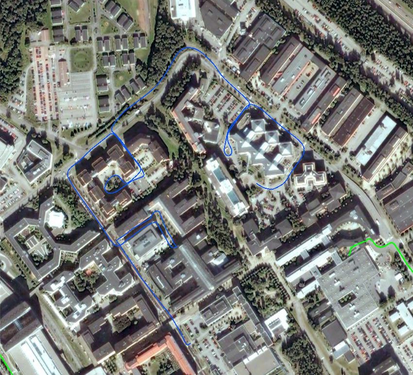
   To experimentally evaluate the proposed method, three               Fig. 13 presents the estimated positions, marked with white,
separate antennas were used to collect measurements in the         on top of the true position, marked with red, for the whole path
Kista area in Stockholm, Sweden. The network mimics a              in the network. In the majority of the trajectory, the estimated
macro-cell deployment of LTE in urban areas. The inter-site        positions follow the true trajectory with high accuracy. How-
distance of BSs were between 350 m to 600 m where the height       ever, in the area x ≈ [500, 600]> and y ≈ [400, 500]> , the
of all the antennas were a few meters above the average height     measurements suffer from NLOS conditions [37]. The poor ac-
of the buildings in the surrounding environment. The synchro-      curacy in some areas of the real network deployment scenario
nization of the transceivers were highly accurate, with standard   is due to both the geometry of the antenna placements and the
deviation of less than 10−12 s. The ground truth trajectory is     MS, and also a result of NLOS effects in the measurements.
obtained by logging GPS measurements. The whole trajectory             The positioning error of the real field experiments is cal-
took 18 minutes to traverse. For more detailed description of      culated relative to the GPS logged positions. Fig. 14 presents
hardware and the measurement campaign see [37]. Fig. 13            the RMSE of the proposed filter bank and of the proposed
presents the taken path.                                           filter bank allowing for a lag of T = 5 s to resolve mode
   The performance of the proposed method is evaluated for         ambiguities. The reported values corresponding to the filter
the experimental scenario in terms of the scatter plot of the      bank are based on the MMSE estimate of the position without
estimated position and the positioning error. The sampling         any further knowledge obtained from the change in the set of
period of the filters for the real data is T = 5 s. The filters    serving BSs. As expected, the error increases when the two
are initialized at the closest BSs with vx0|0 = vy0|0 = 0.         possible solutions are both likely. The estimation error shrinks
The quantities for the initial uncertainties are the same as the   as soon as the set of serving BSs change. Incorporating this
simulation scenario. The observed standard deviations, used        additional information, as in the proposed filtering solution,
11

                               700                                                                         100
                                         True Position           BS3

                                         Estimated Position                                                 90
                               600
                                                                                                            80

                                                                                                            70
                               500
                                                                                                            60

                                                                                                     CDF
    y-pos [m]

                               400                                                                          50

                                                                                                            40
                               300
                                                                                   BS1                      30

                               200                                                                          20
                                                                                                                                    proposed filter, two base stations
                                                                                                            10                      EKF, three base stations
                               100                                                                                                  NWLS, two base stations
                                                                                                             0
                                                         BS2                                                     0   50       100         150           200              250
                                 0                                                                                   Horizontal Positioning Error [m]
                                     0         200              400          600          800
                                                          x-pos [m]                             Fig. 15: Empirical error CDF of the horizontal positioning
                                                                                                error of the KF bank estimator applied to the data from real
Fig. 13: The final KF bank estimates, marked with white, on
                                                                                                experiments, marked with blue. The result of using NWLS
top of the GPS-logged trajectory of the MS, marked with red.
                                                                                                estimator with two base stations is marked with red and the
The three base stations are marked with green.
                                                                                                result of using EKF with three base stations is marked with
                                                                                                black.
                               450

                               400
                                                                                                models. However, linearization without an extremely good
                               350                                                              prior results in poor performances with the considered non-
      positioning errors [m]

                               300
                                                                                                linear measurement models.
                                                                                                   Fig. 15 presents the CDF of the positioning error for the
                               250
                                                                                                proposed filter with two base stations and the EKF using z̃ as
                               200                                                              measurements. Although the 67 % percentile of the EKF reads
                               150                                                              19 m error that is 4 m less than the proposed filter, the 95 %
                               100
                                                                                                percentile of the estimation error of both algorithms is around
                                                                                                40 m. The proposed method is hence marginally worse than the
                                50
                                                                                                standard method, but does at the same time reduce the need of
                                 0                                                              TDOA measurements to half. The poor performance obtained
                                     0    50     100      150         200   250     300   350
                                                              time [s]                          using a standard nonlinear weighted least squares (NWLS)
                                                                                                approach, marked with red in Fig. 15, indicates that Taylor
Fig. 14: RMSE of the estimated position corresponding to
                                                                                                linearization methods do not perform well in this application.
the experimental data, for the state estimates marked with
                                                                                                The NWLS is initialized at the closest BS position and refined
blue, and the estimate that is delayed to obtain more mode
                                                                                                iteratively to estimate the MS’s position.
information marked with black.
                                                                                                                          VII. C ONCLUSIONS
results in a lower RMSE as shown in Fig. 14.                                                       We have proposed a filter bank framework for positioning
   We further evaluate the performance of the proposed filter                                   based on an RTT and a TDOA measurements obtained from
by comparing it to a conventional TDOA approach with                                            two base stations. We first derived the two possible analytical
no measurement ambiguity. In the considered conventional                                        solutions of the intersection of an RTT circle and a TDOA
approach, the positions are estimated using a standard ex-                                      hyperbola. The nonlinear mapping between the collected noisy
tended Kalman filter (EKF) in which the transition of the                                       measurements to the 2D positions of the MS was then ap-
four-component state vector is modeled using a constant                                         proximated using an estimator based on the unscented trans-
velocity model. At each time, the measurement vector of the                                     formation. In order to estimate the MS position from the two
EKF is given by z̃ = [z̃1 , z̃12 , z̃13 ] where z̃1 denotes TOA                                 UT estimates, they were then fed into a filter bank as pseudo-
and z̃ij , i 6= j denotes TDOA. Note, this solution hence                                       measurements of the position of the MS. The filter bank keeps
uses 50 % more measurements than our solution! Hence, this                                      track of all possible solutions until more information is avail-
method solves a much easier problem, as the ambiguities                                         able. While the MS moves through the network, the serving
observed with only two measurements, can be resolved using                                      BS changes through a handover procedure. The additional
the additional measurement. Alternatively, comparisons could                                    information obtained from the handover is then automatically
be made with existing methods proposed in the literature.                                       utilized by the filter bank. The developed method is evaluated
For instance, the authors in [26] propose a method based                                        in terms of RMSE for both simulated network and real-field
on Taylor linearization of TOA and TDOA measurement                                             experiments collected from the network in the Kista area in
12

Stockholm, Sweden. The results indicate good performance                         [22] P. H. Tseng and K. T. Feng, “Hybrid network/satellite-based location
for data from both networks.                                                          estimation and tracking systems for wireless networks,” IEEE Trans-
                                                                                      actions on Vehicular Technology, vol. 58, no. 9, pp. 5174–5189, Nov.
                                                                                      2009.
                                                                                 [23] K. Stanton and C. Aldana, “Addition of p802.11-MC fine timing
                              R EFERENCES                                             measurement (FTM) to p802.1as-rev: Tradeoffs and proposals,” Mar.
                                                                                      2015.
 [1] Y. T. Chan and K. C. Ho, “A simple and efficient estimator for hyperbolic
                                                                                 [24] J. Tosi, F. T. F, M. Santacatterina, R. S. R, and D. F. . P. . D. .
     location,” IEEE Transactions on Signal Processing, vol. 42, no. 8, pp.
                                                                                      doi:10.3390/s17122898, “Performance evaluation of bluetooth low en-
     1905–1915, Aug. 1994.
                                                                                      ergy: A systematic review.” Sensors, Dec. 2017.
 [2] M. D. Gillette and H. F. Silverman, “A linear closed-form algorithm
                                                                                 [25] 3GPP TS 36.355, “LTE Positioning Protocol (LPP),” V.14.4.0.
     for source localization from time-differences of arrival,” IEEE Signal
                                                                                 [26] Y. Jiang, Q. Hu, and D. K. Yang, “A novel position estimation method
     Processing Letters, vol. 15, pp. 1–4, Jan. 2008.
                                                                                      using hybrid TOA and TDOA in AIS,” Journal of Convergence Infor-
 [3] H. C. So, Y. T. Chan, and F. K. W. Chan, “Closed-form formulae
                                                                                      mation Technology, vol. 8, no. 5, Mar. 2013.
     for time-difference-of-arrival estimation,” IEEE Transactions on Signal
                                                                                 [27] M. A. Spirito, “On the accuracy of cellular mobile station location
     Processing, vol. 56, no. 6, pp. 2614–2620, Jun. 2008.
                                                                                      estimation,” IEEE Transactions on Vehicular Technology, vol. 50, no. 3,
 [4] Y.-T. Chan, H. Y. C. Hang, and P. chung Ching, “Exact and approximate            pp. 674–685, May 2001.
     maximum likelihood localization algorithms,” IEEE Transactions on           [28] G. T. 36.211, “Evolved universal terrestrial radio access (E-UTRA);
     Vehicular Technology, vol. 55, no. 1, pp. 10–16, Jan. 2006.                      physical channels and modulation.”
 [5] R. Amiri, F. Behnia, and M. A. M. Sadr, “Exact solution for elliptic        [29] J. Berkmann, C. Carbonelli, F. Dietrich, C. D. C, and W. Xu, “On
     localization in distributed MIMO radar systems,” IEEE Transactions on            3G LTE terminal implementation - standard, algorithms, complexities
     Vehicular Technology, vol. 67, no. 2, pp. 1075–1086, Feb. 2018.                  and challenges (invited paper),” in Proc. of IEEE International Wireless
 [6] W. Xu, M. Huang, C. Zhu, and A. Dammann, “Maximum likelihood                     Communicationsand Mobile Computing Conference (IWCMC), Crete,
     TOA and OTDOA estimation with first arriving path detection for                  Greece, Aug. 2008, pp. 970–975.
     3GPP LTE system,” Transactions on Emerging Telecommunications               [30] H. Rydén, S. M. Razavi, F. Gunnarsson, S. M. Kim, M. Wang,
     Technologies, vol. 27, no. 3, pp. 339–356, Nov. 2016.                            Y. Blankenship, A. Grövlen, and A. Busin, “Baseline performance
 [7] Y. Wang and K. C. Ho, “TDOA positioning irrespective of source range,”           of LTE positioning in 3GPP 3D MIMO indoor user scenarios,” in
     IEEE Transactions on Signal Processing, vol. 65, no. 6, pp. 1447–1460,           Proc. of International Conference on Location and GNSS (ICL-GNSS),
     Mar. 2017.                                                                       Gothenburg, Sweden, Jun. 2015, pp. 1–6.
 [8] Z. Abu-Shaban, X. Zhou, and T. D. Abhayapala, “A novel TOA-based            [31] F. Gustafsson, Statistical Sensor Fusion. Professional Publishing House,
     mobile localization technique under mixed LOS/NLOS conditions for                2012.
     cellular networks,” IEEE Transactions on Vehicular Technology, vol. 65,     [32] S. Särkkä, Bayesian Filtering and Smoothing. New York, NY, USA:
     no. 11, pp. 8841–8853, Nov. 2016.                                                Cambridge University Press, 2013.
 [9] A. Urruela, J. Sala, and J. Riba, “Average performance analysis of          [33] G. Hendeby, “Performance and implementation aspects of nonlinear
     circular and hyperbolic geolocation,” IEEE Transactions on Vehicular             filtering,” Ph.D. dissertation, Linköping University, The Institute of
     Technology, vol. 55, no. 1, pp. 52–66, Jan. 2006.                                Technology, SE-58183 Linköping, Sweden, 2008.
[10] J. Wennervirta and T. Wigren, “RTT positioning field performance,”          [34] S. M. Kay, Fundamentals of Statistical Signal Processing: Estimation
     IEEE Transactions on Vehicular Technology, vol. 59, no. 7, pp. 3656–             Theory. Upper Saddle River, NJ, USA: Prentice-Hall, Inc., 1993.
     3661, Sep. 2010.                                                            [35] N. Bergman, “Recursive Bayesian estimation: Navigation and tracking
[11] A. Ray, S. Deb, and P. Monogioudis, “Localization of LTE measurement             applications,” Dissertations No 579, Linköping Studies in Science and
     records with missing information,” in Proc. of IEEE International                Technology, SE-581 83 Linköping, Sweden, May 1999.
     Conference on Computer Communications, San Francisco, CA, USA,              [36] K. Radnosrati, C. Fritsche, G. Hendeby, F. Gunnarsson, and F. Gustafs-
     Apr. 2016, pp. 1–9.                                                              son, “Fusion of TOF and TDOA for 3GPP positioning,” in Proc. of
[12] J. Yan, L. Zhao, J. Tang, Y. Chen, R. Chen, and L. Chen, “Hybrid kernel          19th International Conference on Information Fusion (FUSION), He,
     based machine learning using received signal strength measurements               Jul. 2016, pp. 1454–1460.
     for indoor localization,” IEEE Transactions on Vehicular Technology,        [37] J. Medbo, I. Siomina, A. Kangas, and J. Furuskog, “Propagation
     vol. 67, no. 3, pp. 2824–2829, Mar. 2018.                                        channel impact on LTE positioning accuracy: A study based on real
[13] L. Cong and W. Zhuang, “Hybrid TDOA/AOA mobile user location                     measurements of observed time difference of arrival,” in Proc. of 20th
     for wideband CDMA cellular systems,” IEEE Transactions on Wireless               IEEE International Symposium on Personal, Indoor and Mobile Radio
     Communications, vol. 1, no. 3, pp. 439–447, Jul. 2002.                           Communications, Westin Toyko, Toyko, Japan, Sep. 2009, pp. 2213–
[14] Y. Qi, H. Kobayashi, and H. Suda, “Analysis of wireless geolocation              2217.
     in a non-line-of-sight environment,” IEEE Transactions on Wireless
     Communications, vol. 5, no. 3, pp. 672–681, Mar. 2006.
[15] A. Mallat, J. Louveaux, and L. Vandendorpe, “UWB based positioning
     in multipath channels: CRBs for AOA and for hybrid TOA-AOA based
     methods,” in Proc. of IEEE International Conference on Communica-
     tions, Glasgow, Scotland, Jun. 2007, pp. 5775–5780.
[16] B. D. V. Veen and K. M. Buckley, “Beamforming: a versatile approach
     to spatial filtering,” IEEE ASSP Magazine, vol. 5, no. 2, pp. 4–24, Apr.
     1988.
[17] H. Krim and M. Viberg, “Two decades of array signal processing
     research: the parametric approach,” IEEE Signal Processing Magazine,
     vol. 13, no. 4, pp. 67–94, Jul. 1996.
[18] C. Chong, C. Tan, D. I. Laurenson, S. McLaughlin, M. A. Beach, and
     A. R. Nix, “A new statistical wideband spatio-temporal channel model
     for 5-GHz band WLAN systems,” IEEE Journal on Selected Areas in
     Communications, vol. 21, no. 2, pp. 139–150, Feb. 2003.
[19] Y. Shen and M. Z. Win, “On the accuracy of localization systems
     using wideband antenna arrays,” IEEE Transactions on Communications,
     vol. 58, no. 1, pp. 270–280, Jan. 2010.
[20] P. H. Tseng and K. T. Lee, “A femto-aided location tracking algorithm
     in LTE-A heterogeneous networks,” IEEE Transactions on Vehicular
     Technology, vol. 66, no. 1, pp. 748–762, Jan. 2017.
[21] G. Wang, Y. Li, and N. Ansari, “A semidefinite relaxation method
     for source localization using TDOA and FDOA measurements,” IEEE
     Transactions on Vehicular Technology, vol. 62, no. 2, pp. 853–862, Feb.
     2013.
You can also read