DLR-IB-MO-HF-2021-40 Modeling of a Generic Cost-Efficient Spare Parts Inventory Management based on a Prognostics and Health Management Approach ...
←
→
Page content transcription
If your browser does not render page correctly, please read the page content below
DLR-IB-MO-HF-2021-40

Modeling of a Generic Cost-Efficient
Spare Parts Inventory Management
based on a Prognostics and Health
Management Approach to Aircraft
Maintenance

Masterarbeit

Maximilian Rammner
Institute Aeronautics and Astronautics
 Chair of Flight Guidance and Air Transport

 — Master Thesis —

 Modeling of a Generic Cost-Efficient Spare Parts Inventory
Management based on a Prognostics and Health Management Approach
 to Aircraft Maintenance

Author: Rammner, Maximilian
Student ID:: 373282

1st Examiner : Prof. Dr. ir. Maarten Uijt de Haag
2nd Examiner : Eric Schuster, M.Sc.
External Supervisor: Robert Meissner, M.Sc. (German Aerospace Center, DLR)

Place, Date: Berlin, 22nd February 2021
Selbstständigkeitserklärung

Hiermit erkläre ich, dass ich die vorliegende Arbeit selbstständig und eigenhändig sowie
ohne unerlaubte fremde Hilfe und ausschließlich unter Verwendung der aufgeführten Quel-
len und Hilfsmittel angefertigt habe.

 Berlin, 22.02.2021
 Berlin, Datum Unterschrift

 i
Kurzfassung

Die Luftfahrtbranche ist durch einen stetig steigenden Wettbewerbs- und damit Kosten-
druck gekennzeichnet, wobei die Fluginstandhaltung einen wesentlichen Kostentreiber dar-
stellt. Die zunehmende Digitalisierung und Automatisierung in der Industrie führt auch
in diesem Sektor zu neuen Instandhaltungstechnologien, wie z.B. PHM (Prognostics and
Health Management). Diese Methoden ermöglichen die Bestimmung des Gesundheitszu-
stands und Vorhersagen über die Restlebensdauer von Bauteilen und können zur Ent-
scheidungsfindung in umliegenden Prozessfeldern beitragen. Die Ersatzteillogistik und das
Ersatzteilmanagement gelten als eines der verwandten Prozessfelder, die von dieser Tech-
nologie profitieren können. Basierend auf dem in der Lagerlogistik weit verbreiteten EOQ-
Konzept (Economic Order Quantity) beschäftigt sich diese Arbeit mit der Modellierung
eines Logistiksystems, das auf der Vorhersagefähigkeit einer PHM-Strategie basiert. Der
entwickelte generische Simulationsrahmen kann sowohl auf Verschleißteile als auch auf re-
paraturfähige Teile durch die Implementierung eines Reparaturzyklus angewendet werden.
Eine simulationsinhärente, iterative Variation der logistischen Größe des Servicelevels und
des Prognosehorizonts, als Kriterium des Technologieniveaus des PHM-Systems, führen zu
einer Optimierung der betrachteten Logistikkosten. Die Anwendung in einer Fallstudie, in
der Eingangskostenverteilungen und Bedarfe variiert werden, führt zur Quantifizierung der
Logistikkosten und zur Abschätzung des Einsparpotenzials im Vergleich zu einer konven-
tionellen Bestandsführungsstrategie nach dem EOQ-Modell.

 Die vorliegende Masterarbeit wurde in englischer Sprache verfasst.

 iii
Modeling of a Generic Cost-Efficient Spare Parts Inventory
 Management based on a Prognostics and Health Management
 Approach to Aircraft Maintenance

 Maximilian Rammner

 The aviation sector is characterized by steadily increasing competitive and thus cost-
 reducing pressure, with aircraft maintenance representing a significant cost driver. Increasing
 digitalization and automation in the industry are also leading to new maintenance technologies,
 such as PHM (Prognostics and Health Management), in this area. These methods enable the
 determination of the condition as well as predictions about the remaining component lifetime
 and can contribute to decision-making in surrounding process fields. Spare parts logistics
 and inventory management are considered to be one of the ancillary process fields that can
 benefit from this technology. Based on the EOQ (Economic Order Quantity) concept widely
 used in inventory logistics, this paper deals with the modeling of a logistics model based on the
 predictive capability of a PHM system. The generic simulation framework developed can be
 applied to expendable parts as well as repairable parts through the implementation of a repair
 cycle. A simulation-inherent, iterative variation of the service level and the prognostic horizon,
 as a criterion of the technological maturity of the PHM system, lead to an optimization of the
 considered logistics cost. The application in a use case study, in which input cost distributions
 and demands are varied, leads to the quantification of logistics cost and the assessment of the
 savings potential by comparison with a conventional inventory management strategy according
 to the EOQ model.

 Nomenclature
 Lead time [d]
Symbols Prognosed time until repair completion [d]
 ( ) MTBF (std. dev.) [fh] Removal margin [fh]
 ( ) MTTR (std. dev.) [d] Prognosed RUL [d]
 ℎ Holding cost [mu] Simulation duration [d]
 Ordering cost [mu] Abbreviations
 Repair cost [mu] Aircraft
 Stock-out cost [mu] Advanced Data Information
 Unit cost [mu] Economic Order Quantity
 ℎ∗ Holding cost unserviceable parts [mu] ℎ Flight Hours
 Demand [1/d] International Air Transport Association
 Discrete demand (single part) [1/d] Integrated Vehicle Health Management
 Demand PHM-based model [1/d] Mean Time Between Failure
 Demand based on desired SL [1/d] Mean Time Between Removal
 Repair capability [-] Mean Time To Repair
 Fleet size [-] Monetary Units
 Probability of stock level [-] Prognostic Accuracy Criterion
 Reorder quantity [-] Prognostics and Health Management
 Reorder point [-] Remaining Useful Life
 Repair supply [1/d] Service Level
 Discrete repair supply (single part) [1/d] United States Coast Guard
 Current time [d]
 1
I. Introduction
 Ever-increasing competitive pressure, a continuing wave of consolidation and epidemic-related effects are forcing air-
lines to reduce cost significantly. One opportunity is the cost item of maintenance, repair and overhaul, which, according
to IATA (International Air Transport Association), represented an average of 9 % of an airline’s operating cost in 2018 [1].

 The PHM (Prognostics and Health Management) concept, which is becoming increasingly influential in the aviation
industry, offers an approach to reduce operating cost while increasing fleet reliability [2]. Currently, planned aircraft
maintenance is mainly based on preventive methods with time- or cycle-based maintenance events and parts replacements
[3]. In the course of digitalization, which is expected to quantify the annual savings potential in aircraft maintenance
to up to $ 3 bn. [4], in combination with the increasing use of methods such as big data, artificial intelligence and
algorithms for decision-making, the potential in maintenance is shifting towards the concepts of predictive - or more
advanced - prescriptive maintenance [5]. While the first predicts the time of failure, prescriptive maintenance enables
targeted solution strategies [6]. The strategies of predictive maintenance and prescriptive maintenance represent
manifestations of the PHM concept, on the one hand as (Prognostics and Health Monitoring, PHM) and on the
other hand as (Prognostics and Health Management, PHM) [2]. The former describes the ability to determine the
state of health, the prediction of occurring failures and the remaining useful life (RUL) [2, 7]. The basis of the
prognosis function is provided by experience-based, data-driven or physical models [8]. The second PHM expression
covers the use of the generated prognosis information for strategic and operational decision-making, which also
affects logistics, for example. This term coincides with the term IVHM (Integrated Vehicle Health Management),
which is also commonly used in the literature [2, 9, 10]. Rodrigues et al. [2] present a global overview of the ben-
efits of introducing PHM technologies on the processes involved in aircraft maintenance, referring to cost-benefit analyses.

 Due to the fact that aircraft maintenance, as the core of the product life cycle management of an aircraft, is closely
linked to surrounding processes, the savings potentials affect surrounding fields such as flight operations or supply
chain management [2]. The latter provides the research scope of the present thesis, which is defined as achieving an
economically sensible balance between the level of service to the customer, the product cost and the capital employed
[11, 12]. A sub-objective is the reduction of capital tied up in inventory [13, 14]. The worldwide annual cost for spare
parts inventory in the aviation industry are quantified at 4.5 - 6.5 bn. US dollars [15].

 Based on concepts of prognostics-based maintenance, the following main hypothesis shall be examined: Efficient
logistics that ensure high parts availability with a relatively low inventory of spare parts can considerably reduce the
total cost of spare parts supply [15]. This paper deals with the modelling of PHM-based inventory management, which
quantifies the logistics cost based on input parameters of the PHM system as well as the logistics itself and shows the
savings potential by comparison with a conventional stocking method. In order to examine the outlined main hypothe-
sis, the following hypotheses are defined concerning the established model and will be evaluated through a use case study:

 ( 1 ) Compared to the conventional model, the proposed model allows a cost reduction by applying the predictions
 of the PHM technology.

 ( 2 ) The higher the quality of the prognostics technology, the longer the possible prognostics horizon, which offers
 a potential reduction in logistics cost.

 ( 3 ) Compared to the conventional model, the proposed model allows a significantly improved logistics performance
 as well as a better cost potential with a random, normally distributed demand, which is indicated by an uneven
 distribution of maintenance activities.

 In order to outline the state of research and identify possible potential with regard to the development of an inventory
model, various publications were reviewed.
For logistical considerations, the determination of demand is considered to be a key issue. Ghobbar and Friend
[16] compare different demand prediction methods based on real flight operational inventory data. Gu et al. [17]
established spare parts inventory management through non-linear programming methodology and determined demand
based on installed parts failure distribution. Zhu et al. [18] discusses the use of an ADI (Advanced Data Information)
to extend the purely statistical time series model of spare parts demand determination. The maintenance plan serves
here as an additional, prognostic source of information for demand. An approach to decision-making in logistics based

 2
on condition-based methods is shown by Zhao et al. [19], where a joint inspection and spare ordering policy was
established. Rodriuges and Yoneyama [20], on the other hand, choose a conventional [R (reorder point), Q (reorder
quantity)] inventory model to show the cost advantage for PHM-based model modifications in terms of reordering
timing in the use case of spare parts stocking for non-repairable items.

 This thesis also adopts the approach of modeling based on an [R, Q] model as well as the methodology for deriving
the reorder point shown by Rodriuges and Yoneyama [20]. Fundamental differences of the model developed within
this thesis, identified as a research gap, are the logistics control also based on PHM technology parameters, the
implementation of a repair cycle and a dynamic reorder quantity. Furthermore unsteady demands are considered.
Another methodological focus is the choice of an iterative, logistics cost-influencing parameter optimization.

 This paper is structured as follows: First, a brief overview of the basics of inventory management is given by the
second chapter. This is followed by a description of the modeling of a simplified PHM model, which provides the basis
for the logistics model presented in chapter III. Here, a subdivision is made between the conventional model and the
PHM-based, proposed model and special focus is placed on the implementation of a repair capability. Chapter IV
presents the established simulation framework, which is used in the subsequent use case study (chapter V) to generate
results and quantify the logistics cost considered and the savings potential. Finally, chapter VI summarizes the findings
of this thesis in terms of modeling a PHM-based inventory management and provides further research potential.

 II. Inventory Fundamentals
 In general, the justification for the necessity of warehousing spare parts, both rotable/repairable as well as expend-
ables/consumables, may be based on the need to maintain the operational readiness of the aircraft fleet, for example, to
avoid cost-intensive delays due to supply shortages in the context of maintenance [17, 21]. This is countered by the cost
driver of overstocking, so that a suitable inventory policy is considered necessary for targeted profitability [21]. The
following cost drivers, which are covered within the proposed model, influence profitability [22]:

 • Ordering cost or procurement cost consist of the direct1 and the indirect procurement cost (fixed order cost),
 for example the administrative costs of the ordering process [21]. In the further context of this thesis, the term
 "ordering cost" is used to refer to the fixed cost.

 • Holding cost or storage cost represents all the cost associated with the storage of the inventory. Included is the
 cost of capital tied up, space, insurance, protection, and taxes attributed to storage [22]. In terms of aviation, there
 are also cost for maintaining serviceability [3].

 • Shortage cost, used in the further proceedings under the term stock-out cost, occur when demand cannot be met
 by stocked parts. Here, the cost development can be differentiated under "backlogging", the holding back of
 demand until it is satisfied, or "no backlogging". In the case of the latter, the cost arise, for example, from rush
 orders that have been placed. [22]

Existing models can be classified according to two further distinctions. The first is the type of inventory replenishment
policy:

 • Continuous Review, where the order is triggered by the stock falling below a critical value [22].

 • Periodic Review, which initiates the ordering cycle and replenishes the inventory up to a defined maximum [22].

The second classification of inventory models refers to the prediction of demand, which can be stochastic and thus based
on statistical, mostly historical data, or deterministic, so that a discrete future demand is predictable [22].

 The EOQ (Economic Order Quantity) model to be considered for the conventional inventory management is
classified as a continuous review, stochastic model. This also provides the basis for the developed PHM-based logistics
 1 ( · )

 3
model, whereby the demand forecast function allows a reclassification towards a more deterministic one.

 The EOQ model fulfils the task of inventory management by determining when and how much to replenish inventory
so at the lowest level of cost [22]. The parameter of the reorder point R is determined from the demand during the
lead time, which is to be seen as the difference between the order trigger and the availability in the stock [21, 22]. In
stochastic models, the demand results from a demand probability density function. A service level can be used to
decide between establishing high safety stocks or accepting shortages [22]. The service level is defined as the expected
probability of not hitting a stock-out during the next replenishment cycle [23].

 The reorder quantity Q is considered to be cost optimized between fixed order cost ( ) and holding cost ( ℎ )
depending on the demand ( ) [21]. Due to the inclusion of the service level, intentional shortages are also possible and
allowed so that the shortage cost ( ) are also considered in the calculation of the reorder quantity. The reorder quantity
results from the following equation, derived in [22]:

 s
 2 · · · ( ℎ + )
 = (1)
 ℎ ·

 The assumption of a constant demand D applies and thus fluctuations cannot be covered [22]. Furthermore, it is
assumed that all ordered parts arrive at the same time [22]. Wongmongkolrit and Rassameethes [24], therefore, offer a
method for modifying the conventional EOQ model to include the consideration of discrete demand. However, the
inclusion of PHM methods offers another potential solution to unsteady demand, which will be addressed in the course
of the paper.

 III. Methodology
 This chapter builds on the foundations laid in the previous part of the thesis to provide an explanation of the logic of
the established model. The basis for the logistics models, conventional as well as PHM-based inventory management, is
provided by the following PHM maintenance model.

A. PHM Model
 Within this sub-chapter, the methodology for establishing a simplified PHM model based on the aircraft health data
is presented. The objective is to generate a prediction of the remaining useful life (RUL) of an aircraft component as a
probability distribution. The following procedure is applied:

 • In order to provide direct comparability with a conventional inventory model, PHM modeling is based on the input
 variable of a mean time between failure (MTBF) with a defined standard deviation of a time-based degrading
 component. The incremental degradation per flight cycle is generated as a function of the flight time and based on
 the specified MTBF with the associated standard deviation as a random value from a generated normal distribution.
 As a result, a new state of health of the aircraft component is obtained per flight cycle.

 • Within this work, component degradation is assumed to be linear.

 • Since the following logistics model is based on a daily inventory analysis, the values for the aircraft health status
 and the prognosed RUL are calculated at the end of daily operation.

 • Assuming the threshold when a failure would occur to be at an aircraft health status of 0 %, the prognosis of the
 point of failure is obtained through interpolation of the obtained values for the health status and extrapolating
 them to a value of 0 %. The resulting point of failure could be transformed into a RUL with the actual amount of
 component lifetime.

 In order to model the deviation of the daily prognostic information, the following procedure is used:

 4
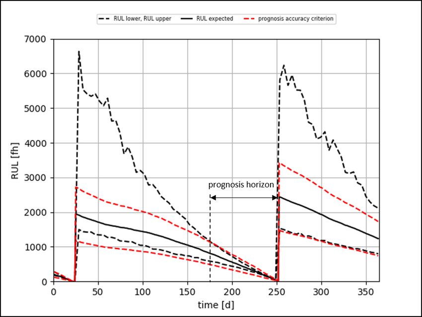
• The aim is to develop a failure probability of the considered component so that, in addition to predicting the RUL
 as a point probability from the discrete health states, a normal distribution is generated.

 • Using the maximum and minimum incremental degradation, the range of future theoretical health states can be
 generated.

 • By interpolating the discrete available health states and these projected theoretical ones, a prediction of minimum
 and maximum RUL can be obtained.

 Figure 1 visualizes this methodology. This graph shows the predicted RUL over the simulation period of a generic
component of an aircraft. The step increase on day 250 indicates the replacement of the component so that the state
of health and thus the predicted RUL is raised again. It can be seen that the bandwidth of the RUL decreases as it
approaches failure.

 Fig. 1 PHM RUL prognosis of one aircraft component over one year

 Furthermore, the inventory logistics will also be investigated based on the influence of PHM technology. For this
purpose, the parameters prognostic accuracy and prognostic horizon are introduced. The first is used in this work as an
input parameter in the form of an evaluation criterion for the technology’s capability. This criterion sets the bounds
around the expected value of the RUL which can be seen in figure 1. The point in time from which the extremes of the
RUL fall within the range defined by the prognostic accuracy criterion (PAC) defines the point in time from which the
prognosis is sufficiently accurate and thus the length of the prognostic horizon.
A high value for the PAC means that the prognosis is considered sufficiently accurate at an earlier point in time than
with a lower value and is thus representative of a higher technological maturity of the PHM system.

B. Inventory Model
 In this work, an inventory replenishment model is used, which follows a continuous review policy, as described
within chapter II. The replenishment is determined by the two variables and . describes the critical inventory
level that triggers a reorder and describes the corresponding reorder quantity. The methodology for determining these
variables for conventional logistics and for proposed logistics, including the information obtained from the PHM, is
described in the following sub-chapters.

 5
1. Modeling Conventional Inventory Control
 The objective of replicating a conventional inventory model is to create a benchmark for the model generated in
relation to PHM technology. As already described above, the theory of the existing EOQ model is used. As discussed in
the previous chapter, with this model it is necessary to determine the reorder point and the corresponding order quantity.
This is done in the reference model on the basis of statistical data which can be derived from the maintenance history.
The conventional EOQ model, which does not consider a repair cycle, determines the reorder point from the demand
probability density function as a function of the desired service level [22].
Including a repair cycle, a part of this demand is covered by the repair supply. The modifications of the EOQ model
introduced in chapter II in the course of implementing a repair cycle are considered subsequently:

Reorder Point For the calculation of the reordering time, the generation of the supply probability density function,
which is composed of the following parameters, is initially considered:

 1) - The number of repair shops, as a resource indicator for the number of independent, parallel repair processes.
 2) - The mean time to repair, and its standard deviation that reflects the duration of a repair process.

 The mean time to repair ( ) is assumed for the repair time. In the conventional model, there is no tracking of the
repair process and therefore the statistical mean value is the best possible assumption. The repair supply is therefore
calculated as:

 = (2)

 This relationship represents the average repair rate in components per day, which is subsequently used to correct the
demand arising from the failures with the aim of generating a demand probability density function taking into account
the following parameters:

 1) - The fleet size, as a measure of the number of homogeneous components, one considered per aircraft.
 2) - The mean time between failure, and its standard deviation that reflects the average component lifetime
 between failures.
 3) - An overall service level, as defined in the fundamentals, chapter II, replicating the probability that no
 stock-out will occur during the subsequent replenishment process.

 Applying the relationship from equation (2), total average demand can be expressed as follows:

 = − (3)

 Through this demand, including the adjusted standard deviation, a demand probability density function is generated
as normal distribution and the demand is determined depending on the selected service level. The reorder point,
expressed as stock level, can be calculated using the average lead time [22]:

 = · (4)

Reorder Quantity As already discussed in chapter II, the economic reorder quantity represents an optimal compromise
between order cost for triggering an order process, holding, and stock-out cost. Its validity is underlined by the assumption
of a constant demand rate. In this model, which serves as a benchmark model for the proposed one, the modified
EOQ (Economic Order Quantity) formula is used, which takes planned shortages into account. This circumstance is
considered reasonable from a management perspective, for example, if the holding cost are relatively high compared to
the default cost [22]. Equation (1) is used in order to calculate the economic order quantity. Taking into account the
supply of repairs, demand D will be expressed by equation (3).

2. Modeling of PHM-based Inventory Control
 While the conventional model is based on statistical quantities to develop a demand probability distribution and thus
the parameters of the inventory model, the prediction from the PHM allows for a failure probability of each individual

 6
component and thus a discrete demand. This fact allows for a precise determination of the parameters of the reorder
point and the assigned order quantity.

Reorder Point The principle that the reorder point is determined from the demand during the lead time does not
change compared to the conventional model. However, in this model the service level, which is defined as the probability
that no stock-out occurs, is used as a trigger for a reorder, as it has been applied in the method according to Rodriuges
and Yoneyama [20].
The model allows for a calculation of the daily service level achieved. The reordering is done in such a way that the
achieved service level is always above the predefined one. Methodologically, the duration of the lead time is projected
into the future to determine the current service level. If the service level falls below a threshold at time + + 1, the
reorder is triggered. This guarantees that the current service level at time + does not fall below the predefined one
and thus a defined service level is guaranteed to be maintained. At time + + 1, the specific failure probability
of each component can be determined from the failure probability distributions originating from the PHM module.
Depending on the currently available stock, the current service level results in the probability that a maximum number
of parts will fail [20]. The method is extended so that a repair is also taken into consideration. Similar to the prediction
of failure probabilities, the PHM module provides a probability distribution of the prediction at which time a component
will be repaired. This circumstance affects the calculation of the current service level in that the stock level increases
with a certain probability at time + + 1. The calculation of the service level is explained below using an established
example scenario:

 Fig. 2 Example scenario PHM-based inventory management

 Figure 2 shows the failure probabilities of the same component per aircraft (AC 1 - AC 5). Furthermore, the
probabilities with which a repair of a component per repair shop (Shop 1 - Shop 2) will be completed are shown. The
gray box visualises the total prognostic horizon. This means that only these components can be taken into account for
the logistics calculation, as the prognosis is defined as sufficiently precise according to the . For the service level at
time , the individual probabilities of occurrence at time + + 1 are determined from the PHM system. Table
1 summarises these for the given example scenario. AC 1 is out of scope because the failure range is not within the
prognostic horizon.

 Table 1 Probabilities of occurance for service level calculation

 Resource AC 1 AC 2 AC 3 AC 4 AC 5 Shop 1 Shop 2
 Probability out of scope 0.0 0.1 0.4 0.9 0.8 0.0

 7
There is one part in stock. Neglecting a repair, the service level results from the probability that at most one part
will fail. From the combinatorics using the probabilities of occurrence from the table, a service level of 58.2 % would
result. Extended to the procedure described in Rodriuges and Yoneyama [20], this changes as follows by including the
repair prognosis: With a probability of 80 %, SHOP 1 delivers a repaired part, so that consequently with a probability of
80 % a stock of two parts will be available at the time considered. For this case, the calculation of the service level
would be the probability of a maximum of two components failing. The probability of this is calculated at 96.4 %.

 Equation 5 represents the calculation of the total service level in the universal form, where n is the sum of stock
and the number of repair shops, is the probability with which a certain stock level occurs and is the associated
service level considering this stock level:

 Õ
 = ( = ) · ( = ) (5)
 =

 In regard to the example presented here, the service level is obtained as follows (equation 6):

 = 0.2 · 0.582 + 0.8 · 0.964 = 0.8876 (6)

 If the specified service level to be maintained were 90 %, this shortfall, according to the service level achieved of
88,76 %, would result in an order being triggered.

Reorder Quantity For the modeling of conventional inventory logistics, the EOQ formula is used, which is based on
the assumption of constant demand. Since this is not always the case in reality, this model quickly reaches its limits.
Hence, the prognostic capability from PHM is used to discretize the demand depending on the prognostic horizon. The
discrete demand results from the number of "visible" prognostic failures and repair completions within the established
prognostic horizon, as depicted in figure 2. For the purpose of simplification, the failure and repair prognoses are
considered as point probabilities in contrast to the determination of the reorder point.

 In principle, demand is calculated as the ratio of the difference between failures and repairs and the duration of the
discrete demand framework. This describes the time frame in which the predicted demand can be satisfied by order at
the current time . In order to pay attention to the sequence of failures and repairs, to reduce additional failure potential,
a weighting method is applied.

 The procedure takes into account all projected failures within the prognostic horizon spanned by the selected
prognostic accuracy criterion. However, this prognostic horizon is corrected by the lead time, since a reorder at time
will not arrive before + + 1. For each forecast failure (index ), the discrete demand ( ) can be assumed as the
following expression (equation 7), where represents the RUL in days of the respective component:

 1
 = (7)
 − ( + 1)

 The same applies to the discrete repair supply ( ) of a visible repair completion (index ), where represents the
time until the repair completion within the respective repair shop:

 1
 = (8)
 − ( + 1)

 8
Assuming m is the number of visible failures and n is the number of visible repair completions within the prognostic
horizon, a weighted demand ( ℎ ) can be derived according to the following formula (equation 9) using the results
obtained from the two equations above:

 Í Í
 − =1
 (9)
 =1
 =
 +

 With reference to the example scenario in figure 2, three failures and one repair completion can be predicted within
the discrete demand time frame. The following values for reliably forecast failures (AC 2, AC 3, AC 4) and repair
completion (SHOP 2) within the discrete demand frame, assuming a lead time of = 10 and the given, exemplary
values for and , can be calculated as follows:

 • AC 2: = 17, 2 = 0.1667
 • AC 3: = 13, 3 = 0.5
 • AC 4: = 12, 4 = 1.0
 • SHOP 2: = 15, 2 = 0.25

 Using equation 9, a demand of = 0.354 can be determined.

 This calculated demand is used in the reorder quantity-equation (equation 1). The result is rounded up to an integer.
Instead of using an average, statistics-based demand, the proposed model uses a demand as a function of the prognostic
horizon. Furthermore, two limitations are set up:

 • The minimum reorder quantity is one item in order to comply with the required service level.

 • A maximum results from the number of predicted failures. This limitation applies when the value of
 according to the EOQ formula with the demand exceeds the amount of forecast failures. Furthermore it
 opens up advantages over the conventional methodology in that costs can be reduced in the case of uneven demand
 distribution.

 IV. Simulation Framework
 After the theoretical foundations and methodologies behind inventory logistics model and its underlying PHM
model have been explained, the following section presents the structure and process of the simulation of inventory
management including the cost calculation based on a PHM system in aircraft maintenance. It should be emphasized
that this simulation has a generic character and represents reality in a limited way only. Rather, this work aims to
conduct research into the relationship between a PHM strategy and the resulting logistics cost.

A. Simulation Scope and General Process
 The general scope of the simulation can be gathered from figure 3. The stakeholders of the simulation scenario are
shown as well as the material flow of the logistics. The parts warehouse, maintenance, and repair shop are physically
united in one place in order to simplify the simulation. The procurement of spare parts is provided by a single supplier
and possesses a certain lead time. Furthermore, it is possible to repair dismantled components so that they are available
again after a certain time.
 The aircraft operate according to a randomly generated flight schedule which determines the number of legs to be
flown daily and a dependent flight time according to the following pattern (table 2):

 An even number of daily legs was chosen to ensure that the aircraft always return to their base at the end of the
day. The evaluation of the health conditions and determination of the RUL prognosis, a possible maintenance event, as
well as the control of the logistics including order triggering is done on a daily basis at the end of the respective day of

 9
Fig. 3 Simulation scenario

 Table 2 Flight schedule pattern

 Legs [-] 2 4 6
 Flight time range [fh] 4-6 2.5 - 4 0.5 - 2.5

operation. The following general assumptions (A) have been made:

 ( 1 ) A maintenance event in the form of a replacement of the considered component is triggered as soon as
 the forecast RUL falls below a threshold value. This ensures that the replacement is realized as a planned
 maintenance measure before a component failure.

 ( 2 ) A maintenance task is carried out between two days of flight operations and therefore does not require any
 further layover time. If the required component is available in stock, it is taken from the stock and installed on
 the aircraft. Otherwise, the aircraft remains on the ground until a component is available. There are stock-out
 cost on a daily basis. No rush shipments will be considered.

 ( 3 ) The removed component goes to a repair shop if a free resource is available. Otherwise, it is kept in storage
 until a shop becomes available and causes corresponding daily holding cost.

 ( 4 ) In the repair shop, repair cost incur daily. Upon completion, the part leaves the shop and increases the stock in
 the warehouse. Besides, there is a daily prognosis of the expected time to completion based on incremental
 progress, which is used in the proposed PHM-based inventory model.

 ( 5 ) Within this model, it is assumed that the cost of a repair is far less than the cost of a reorder. This is the case
 due to the fact that a repair always takes place as soon as a resource is available in the form of a shop.

 ( 6 ) An ordering process causes fixed ordering cost as well as variable cost in the form of the price of the new part
 itself.

 ( 7 ) The lead time is constant for all orders.

 ( 8 ) Holding cost incur for the storage of all components, i.e. airworthy and scrapped, in the warehouse. There
 is a consideration of higher holding cost for airworthy parts, caused by higher capital tie-up cost and the
 maintenance of serviceability.

 ( 9 ) If the simulation specification of the model does not allow for repair, as it is the fact within the third scenario
 of the developed use case study, no disposal cost are considered for replaced, unserviceable parts.

 10
( 10 ) If a delivery or repair completion of a component takes place on the same day for installation, no holding cost
 are due.

B. Simulation Process
 Based on these assumptions about the model, the program was implemented in Python, with the described
functionalities outsourced to functions and modules. The methodology is generally a discrete-time simulation on a
daily basis, though the flight operation including component degradation was implemented as a discrete-event simulation.

 Fig. 4 Simulation process diagram

 Figure 4 summarizes the executed model functionalities in a simulation process diagram. In principle, the
conventional, as well as the proposed inventory model, are simulated simultaneously based on the described PHM
maintenance strategy, so that comparability is guaranteed. In the context of the following use case study, reference
should be made to the user input and the output of the simulation model.

 In general, there is a choice of simulation time and the number of aircraft. One generic component per aircraft is
considered, for which an MTBF including a standard deviation is specified. Based on these parameters, the degradation
is simulated within the PHM model and the conventional inventory logistics are controlled. An hourly time can be
specified via an additional removal margin so that an MTBR (Mean Time Between Removal) can be derived from
the MTBF since according to the assumptions made above, a component replacement is to be considered before
failure. Furthermore, there is a query whether a repair in the shop should be considered. If this is the case, an MTTR
is selected including the standard deviation and the number of shops that guarantee a simultaneous repair as well
as the repair cost on a daily basis. The choice of the cost for a new component is followed by the selection of logistics cost:

 11
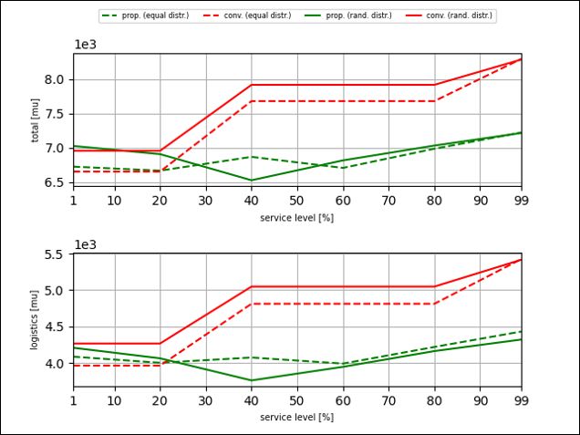
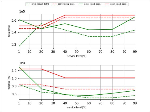
There are stock-out and holding cost on a daily basis. In the latter case, a distinction is made between holding
cost for a new part and an unserviceable part. This allows for higher holding cost for new parts, due to the servicing
requirements to retain the components airworthiness [3]. Fixed ordering cost are considered for each ordering process.
To maintain the generic character of the model, the unit of cost is monetary units so that the absolute size is less
important than the relation to each other. Furthermore, the lead time is chosen as a logistical parameter.

 The final user input is the limitation of the control variables to be investigated, which are the focus of this work. The
first is the prognostic accuracy criterion, which has a direct influence on the prognostic horizon and, as explained in
chapter III, reflects a PHM technology capability, and a specification for the service level. The latter implies the size of the
safety stock, i.e. the level of accepted stock outs according to the considerations made in chapters II and III. Depending
on these variables, the minimum cost for spare parts stocking are to be determined. Thus, there is no preselection of a
discrete value, but a range of values including a step size for both parameters. The simulation allows a parallel variation
of each of these parameters in the daily simulation step so that the model performs an iterative cost calculation for each
parameter combination, depicted within figure 4, while at the same time ensuring comparability. This optimization
approach allows the minimum logistics cost to be determined as a function of the control variables mentioned. A third
control variable is the type of failure distribution, which is directly related to the demand for required spare parts. This was
introduced mainly to show the limitations of the conventional EOQ inventory model, as the application of EOQ is related
to a constant demand distribution. The proposed inventory model’s advantage, due to its prognostic capability, is that it
can react to dynamic fluctuations in demand. As a result, the user can choose between three modes of demand distribution:

 • Equal distribution of demand
 • Random distribution
 • Stepwise selectable demand peaks

 The choice of these parameters will now be dealt with directly in the course of the description of the initialization
process for starting the simulation. At the start of the simulation, all the components considered are given an initial
health status and a dependent previous flight time for each aircraft. The mode selected by the user for the distribution of
demand is thus pre-controlled via the initial health states. If, for example, all initial health states within the considered
component are close to each other within the fleet, this results in a strong fluctuation in demand for spare parts over the
simulation runtime. Furthermore, the repair shops are initialized with random initial repair progress and the initial stock
level is set.

 Regarding the output, first, the history of the stock of serviceable spare parts for both the conventional and the
proposed model can be compared. From this, order times, goods receipts from the supplier, and the repair shop as well
as shortages and related delays can be derived. Second, the total cost, as well as the pure logistics cost for the simulation
period, are presented. This is done for the conventional model depending on the selected range of the service level. For
the proposed inventory model, the evaluation and presentation are carried out using the service level as well as the
prognostic accuracy criterion. A split of the individual cost as shares of the total cost is provided as well.

 V. Use Case Study
 Based on the described simulation process and the theoretical model fundamentals, a demonstration is carried out
in the form of this use case study. The aim is to compare the logistics models concerning their resulting cost and to
examine the hypotheses made. In the course of this work, three scenarios were designed that represent the spare parts
logistics of three generic components by varying the cost and the component lifetime. For each of these scenarios, the
demand distribution is varied between the options of an ideal uniform demand distribution and an unsteady distribution,
as described in chapter IV. This results in three scenarios that form the basis of the cost variation, each with a case
distinction in the demand distribution, thus six cases. The total cost, as well as the pure logistics cost for each of these
cases, are evaluated for the conventional inventory model as well as for the developed logistics model adapted to the
PHM technology. As already mentioned in the context of the simulation framework, the cost development for the former
is dependent on the service level and for the latter additionally on the prognostic accuracy criterion. Figure 5 shows the
subdivision of the use case study, which is conditionally equivalent to a sensitivity analysis:

 12
Fig. 5 Use case study - parameter variation

A. Simulation Input Parameter
 Global, scenario-homogeneous simulation parameters are provided in table 3. The derivation of the scenario-specific
input variables is covered within the next three subchapters.

 Table 3 Global, scenario-homogeneous simulation parameters

 Parameter Description Value Dimension
 Simulation duration 365 [d]
 Fleet size 20 [-]
 Removal margin 16 [fh]
 Lead time 20 [d]
 Service level 1 - 99 [%]
 Prognostic accuracy criterion 2 - 14 [%]

1. Scenario I
 The first scenario is intended to depict the inventory management of a rotable, price-intensive component. Signifi-
cantly, high stock-out cost, as well as a low inventory level, should be represented.

 In the context of determining the cost distribution of the input variables as well as the lifetime of the generic
component, real data of a component from the literature are initially used, which meet the requirements of the first
scenario. Based on this cost distribution, missing cost items can be estimated or completely varied to obtain a cost
distribution for the second scenario. This type of estimation and the expression of cost in monetary units preserve
the generic character of this use case. The aircraft maintenance and inventory databases of the United States Coast
Guard (USCG) provides cost and component life data of the main gearbox of the aircraft type HH65A [25]. These
data are further adopted for Scenario I according to table 4. According to the assumptions made, the holding cost for a
non-serviceable part are 25 % of those of a serviceable part. The parameters of the repair cycle and the administrative
ordering cost are to be determined. The former, also apparent in table 4, were estimated on the assumption that the
repair supply is significantly lower than the demand, as explained in chapter IV. Here as well as within the second
scenario, the values of the repair capacity are determined in such a way that 25 % of the demand can be covered by
the repair. Furthermore, the repair is significantly more inexpensive than ordering new parts, as the decision-making

 13
process between repair and ordering new parts was not considered in this model, but rather the occupation rate of the
available repair resources is always 100 %, if removed parts are available. A value of 25 % of the new component cost
was assumed for the total cost of a component repair. The missing cost item of the order cost is calculated with the help
of the EOQ formula using all assumed variables and the specification of a target order quantity. This default value
for , which is used exclusively to estimate the ordering cost based on all other parameters, is set to 1.25 since this
scenario considers a cost-intensive component for which in practice it is more likely to be stocked in a small quantity.
All assumed scenario-specific input variables are provided in table 4.

2. Scenario II
 In the second scenario, compared to Scenario I, a lower-cost component with a reduced mean time to failure is
considered. The number of repair shops is increased to two, while the measure of repair capacity remains constant
according to the assumption outlined in Scenario I. By choosing new cost ratios based on the previous study case, the
main aim is to reduce the cost impact of the stock-outs. The ordering cost are selected according to the same procedure
by specifying a target order quantity, which is set to 2.25 to consider a certain middle ground between the previous and
the following scenario.

3. Scenario III
 The last scenario aims to consider a consumable component without repair. Compared to the previous scenarios, the
component lifetime is further reduced so that a higher component demand can be reflected. The relative influence of the
stock-out cost is further decreased compared to the last scenario. The values for the component price, the ordering, and
holding cost were taken from an IATA source [26] using the example of a gasket and were also recorded in table 4. The
relative influence of the stock-out cost is further decreased compared to the holding cost. In contrast to the previous
process, the target order quantity is no longer used as a default value for determining the cost distributions but results
directly from it.

 Table 4 Scenario-specific input parameters

 Value
Parameter Description Dimension
 Scenario I Scenario II Scenario III
 Component lifetime
 Mean time between failure 2,436 [25] 1,220 750 [fh]
 Standard deviation 659 [25] 113 69 [fh]
 Repair shop
 Repair capability 1 2 - [-]
 Mean time to repair 45 45 - [ ]
 Standard deviation 12 12 - [d]
 Cost allocation
 Unit cost 500,000 [25] 10,000 25.6 [26] [mu]
 Repair cost (per day) 3,125 56 - [mu]
 ℎ Holding cost (per day) 342 1 71 1.92 2
 ℎ∗ Holding cost unserviceable part (per day) 86 2 - [mu]
 Stock-out cost 6,849 3 68 4 3.2 5 [mu]
 =50 Order quantity (SL = 50 %) 1.25 2.25 7.62 [-]
 Ordering cost 2,893 89 120 [26] [mu]

 1 0.25· 2 3 5.0· 4 2.5· 5
 ℎ = 365 [25] ℎ = 0.075 · [26] = 365 [25] = 365 = 0.125 ·

 14
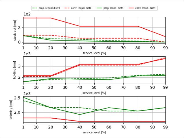
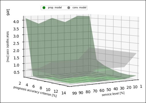
B. Simulation Results
 The following evaluation analyzes the developed use cases according to their resulting logistics and total cost
depending on the input parameters. Furthermore, the inventory development is analyzed over the simulation period.
The evaluation of the first scenario as a reference scenario is carried out in more detail than the following scenarios so
that various correlations of the parameter variation and the capacities of the designed model are shown and discussed at
this point. This is contrasted by a more summarized, cost-oriented evaluation of the other two scenarios. Finally, the
results of the entire use case are summarized, including the findings and limits of the model. It should be emphasized
that within the use cases, a simulation-inherent optimization of the logistics cost, consisting of a stock-out, ordering, and
holding cost for new, serviceable components, is considered. The consideration of component cost, repair cost and the
storage of removed, unserviceable components falls within the scope of the simulation, but not within the scope of
cost optimization and the proposed savings potential to be achieved by the PHM-based inventory management model
compared to the conventional one.

1. Scenario I
 Recapping, the first scenario is characterized as a consideration of the inventory management of a cost-intensive
component, which is supposed to be stocked in small quantities and leads to high stock-out cost in the event of a shortage.
Before the output concerning cost-driving variables and the cost per se of the logistics models to be compared is carried out,
the cost optimization, as well as the development of the inventory over time, is to be discussed exemplary for this scenario.

 Similar to the conventional logistics model, the PHM-based model is also based on the input parameter of the service
level, which, despite different implementation philosophies (see chapter III), is considered the decisive parameter for
the safety stock and thus for avoiding stock-out cost. As already discussed, this is not fixed, but iterated within the
simulation process to find the best set of parameters concerning logistics cost. Besides, these cost of the proposed
model, in contrast to the conventional model, are dependent on the prognostic horizon, represented by the input value of
the PAC. Consequently, this parameter is included in the iterative cost optimisation.

 Fig. 6 Total logistics cost over SL & PAC (input: random distribution) - scenario I

 Figure 6 visualizes the result of this optimization by depicting the distribution of logistics cost as a function of these
variables. As outlined, the cost of the conventional model only change along the axis of the service level and those of
the proposed model depend on both parameters. It can be seen that a large part of the cost area of the PHM-based model
undercuts that of the conventional model. The sensitivity to the selected service level is examined later in the evaluation.
Rather, a high change in sensitivity along the selected, sufficient prognostic accuracy becomes recognizable. Regarding

 15
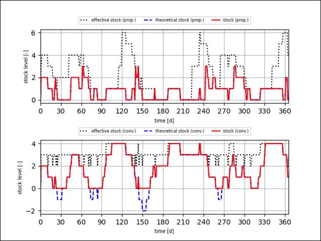
the considerations stated in chapter III, an increase in PAC is associated with an increase in the prognostic horizon, in
which the discrete demand becomes visible and which thus serves as the basis for controlling logistics. Since different
technological capabilities were not implemented in the PHM modeling per se, a high value for the PAC is derived as a
high level of technological maturity. The enormous increase in cost in the direction of a low PAC can be explained by
the fact that at a certain point the length of the resulting prognostic horizon falls below the duration of the lead time and
thus the basis for predicting the reorder time of the PHM-based logistics model is no longer given, which ultimately
manifests itself in high stock-out cost.

 Hypothesis 2 , can be confirmed in principle, although it should be emphasized that the resulting cost initially
have a high sensitivity for the reasons mentioned, but a low sensitivity with increasing PAC and thus technology level.
However, a minimum of sufficient accuracy of the PHM technology, here PAC = 4 % (table 5), is necessary to undercut
the cost of the conventional model. The same table also provides the values for the best-case solution:

 • Conventional model (equal distribution): SL = 20 %
 • PHM-based model (equal distribution): SL = 99 %, PAC = 14 %
 • Conventional model (random distribution): SL = 80 %
 • PHM-based model (random distribution): SL = 80 %, PAC = 8 %

 Prior to referring to the further simulation results presented within this table, the development of the spare parts
stock is exemplary shown for this respective best case of the simulation of the first scenario under the assumption of a
random distribution of the initial health states based on figure 7.

 Fig. 7 Inventory history (optimum PAC & SL, input: random distribution) - scenario I

 The actual stock in the warehouse is expressed by the red line. The blue line depicts the theoretical stock so
that it is an indicator for the stock shortage and thus for the stock-out cost that occur as a result of backlogging.
The effective stock serves as a controller for the order trigger, as it already includes the number of parts ordered
but not yet delivered [20]. In the chart, this is expressed by the increase in the effective stock and after the lead
time by the increase in the stock level, as the part has then been delivered. An increase in the stock level without
a previous increase in the effective stock, for example, visible in the first subplot on day 187, indicates a repair completion.

 Comparing both time series of the stock, it is noticeable that the conventional model has a larger quantity in stock

 16
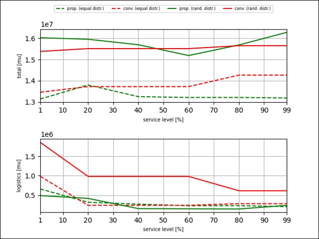
over a longer period. Furthermore, there are occasional longer stock-outs, whereas the proposed model has no stock-outs.
Since the conventional model works with an average demand concerning the reorder quantity, frequent orders are placed
for small quantities, whereas the reorder quantities in the proposed model are more dynamic and thus orders are placed
less frequently. One reason for the low performance of the conventional model compared to the proposed model is the
representation of an inconsistent demand distribution, which is more in line with reality but, as discussed in chapter II,
outside the scope of the convectional EOQ model. It can be noted at the outset that the performance of the conventional
model is better for equal distributions, and thus the performance, as well as cost difference between the models, is
smaller under this simulation condition.

 This fact also becomes evident in the tables 5 and 6, which summarize the absolute cost and relative shares of the
individual cost units and show the relative savings potential, as well as within the figure 8 and 9, which are referred to in
the following.

 Fig. 8 Total cost & total logistics cost over SL (optimum PAC) - scenario I

 Looking at figure 8, the second subplot compares the logistics cost considered in terms of optimization above the
service level of the conventional and PHM-based model in two simulation runs. One with constant demand and the
other with unsteady demand.
It is noticeable that the logistics cost of the conventional model are more sensitive to the service level than those of the
proposed model, which is due to the different model logic. Long constant trajectories of the graphs of the conventional
model can be justified by the fact that the service level achieves a reorder point in the form of a critical stock level. This
is always an integer and consequently only changes with larger service level changes in the case of small quantities to be
stocked. Based only on the input parameters in the previous sub-chapter, a cost optimum of the conventional model
in its regular scope (equal distribution) would have been expected in regions with a high service level. However, an
optimum at a service level of 20 % indicates that allowed delays are not too important compared to other cost cost. This
expectation is reflected in the course of the conventional model under unsteady demand, since fluctuations in demand
are not directly covered by that model. Hence, cost minimization is only accompanied by maximum safety stock and
thus maximum service level.

 The high cost-saving potential between the models becomes visible as a result of the simulation with an uneven
demand (random distribution) of 75.72 % and the more minimal as a result of the simulation with an equally distributed
demand of 13.88 % (table 6) for the respective optimal case.

 17
In addition, the same figure provides a supplementary breakdown of the total cost of the simulation. The cost
curves must be considered under the condition that this work is about optimizing the logistics cost and not the total cost.
Although the savings in logistics and thus the cost advantages are also perceptible in the presentation of total cost, this
graph must always be interpreted in combination with the simulation results from table 5. Here, the total number of
ordered quantities, the maintenance activities, and the repair completions are considered cost drivers for the cost not
considered within the logistics cost optimization. The following reasoning is applied to this scenario:
Based on the observation that the cost savings in terms of logistics cost and thus the spread is greater for the "random
distribution" simulation than for those with "equal distribution", it might be assumed that this fact should also be
reflected in the total cost.
However, the column "Parts ordered" reveals that the total number of ordered parts varies during the simulation pe-
riod and therefore does not allow direct comparability, respectively table 5 must be included in the interpretation of the cost.

 Fig. 9 Logistics cost breakdown over SL (optimum PAC) - scenario I

 A more detailed look at the logistics cost to be optimized concerning the model is provided in figure 9.
Here, the progressions along the service level are also shown. With regard to the stock-out cost, as in the total logistics
cost, the decrease with an increase in the service level is noticeable. The curves of the conventional model prove to be
more sensitive to this. The significantly higher cost for the simulation with unsteady demand for the conventional model
are in line with the comments made concerning figure 7.

 Regarding the holding cost, an increasing trend can be observed with an increase in the service level. A significant
cost difference emerges under the less service level-sensitive courses of the order cost. Taking the cost-driving parameters
from table 5 into account, the differences can be derived based on the average reorder quantity and thus the number of
orders for the respective logistics cost-optimal case.

 Concerning the cost driver of stock-out cost, this table offers another interesting finding: Comparing the values
for the stock-out index of the PHM models for both simulation conditions, it can be assessed that for a lower service
level (80 %) a lower stock-out index (stock-out index = 1) can be achieved than for a higher service level (99 %) with
a stock-out index of 13, whereby higher service levels should obviously result in lower stock-out rates. A possible
explanation is offered by the additional consideration of the , which shows significant differences here and thus
suggests a possible indicator of the sensitivity of the stock-outs concerning the prognostic horizon.

 18
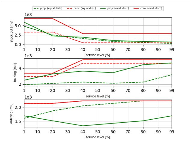
You can also read