Fast character modeling with sketch-based PDE surfaces
←
→
Page content transcription
If your browser does not render page correctly, please read the page content below
Multimedia Tools and Applications
https://doi.org/10.1007/s11042-020-09060-9

Fast character modeling with sketch-based
PDE surfaces

Lihua You 1 & Xiaosong Yang 1 & Junjun Pan 2 & Tong-Yee Lee 3 & Shaojun Bian 1 &
Kun Qian 4 & Zulfiqar Habib 5 & Allah Bux Sargano 5 & Ismail Kazmi 6 & Jian J. Zhang 1

Received: 19 July 2019 / Revised: 6 April 2020 / Accepted: 8 May 2020

# The Author(s) 2020

Abstract
Virtual characters are 3D geometric models of characters. They have a lot of applications in
multimedia. In this paper, we propose a new physics-based deformation method and efficient
character modelling framework for creation of detailed 3D virtual character models. Our
proposed physics-based deformation method uses PDE surfaces. Here PDE is the abbrevia-
tion of Partial Differential Equation, and PDE surfaces are defined as sculpting force-driven
shape representations of interpolation surfaces. Interpolation surfaces are obtained by inter-
polating key cross-section profile curves and the sculpting force-driven shape representation
uses an analytical solution to a vector-valued partial differential equation involving sculpting
forces to quickly obtain deformed shapes. Our proposed character modelling framework
consists of global modeling and local modeling. The global modeling is also called model
building, which is a process of creating a whole character model quickly with sketch-guided
and template-based modeling techniques. The local modeling produces local details efficient-
ly to improve the realism of the created character model with four shape manipulation
techniques. The sketch-guided global modeling generates a character model from three
different levels of sketched profile curves called primary, secondary and key cross-section
curves in three orthographic views. The template-based global modeling obtains a new
character model by deforming a template model to match the three different levels of profile
curves. Four shape manipulation techniques for local modeling are investigated and integrat-
ed into the new modelling framework. They include: partial differential equation-based shape
manipulation, generalized elliptic curve-driven shape manipulation, sketch assisted shape
manipulation, and template-based shape manipulation. These new local modeling techniques
have both global and local shape control functions and are efficient in local shape manipu-
lation. The final character models are represented with a collection of surfaces, which are
modeled with two types of geometric entities: generalized elliptic curves (GECs) and partial

Electronic supplementary material The online version of this article (https://doi.org/10.1007/s11042-020-
09060-9) contains supplementary material, which is available to authorized users.

* Lihua You
  lyou@bournemouth.ac.uk

Extended author information available on the last page of the article
Multimedia Tools and Applications

differential equation-based surfaces. Our experiments indicate that the proposed modeling
approach can build detailed and realistic character models easily and quickly.

Keywords Virtual characters . Model building . Sketch-guided global modeling . Template-based
global modeling . Local modeling techniques . Generalized elliptic curves . PDE surfaces

1 Introduction

Modeling of virtual characters is essential in many multimedia applications. Various sketch-
based, template-based, and physics-based methods have been developed to raise efficiency,
increase details, and improve realism of virtual character modeling.
   Sketch-based modeling creates 3D models from freehand drawings. It tackles the
weaknesses of heavy manual operations and low modelling efficiency met by mainstream
3D modelling animation packages such as Maya and 3D Max. A main problem for sketch-
based modeling is how to generate detailed and realistic 3D models. Sketching from a
single view cannot provide the shape information in other views. Due to this reasons, most
sketch-based modeling systems [18] sketch from many views with a workflow “sketch-
rotate-sketch” [12]. For such a workflow, how to find a good view for a stroke is often
difficult and time-consuming, and due to the changes, users cannot match their input
strokes to a guided image as pointed out in [12]. Creating an isometric view from a
standard 3-view orthographic drawing avoids the difficulty of finding good views and has
been popularly applied in engineering drawing and design [29]. It has also been used to
create 3D man-made models [34]. However, one main limitation for this approach is with
3D organic models such as character models where a majority of facets share no common
axes. Another limitation is it does not follow the “coarse-to-fine” workflow of organic
modeling. The approach proposed in this paper is motivated by using three orthographic
silhouettes of the whole model and its part models, but uses a stepwise approach to suit the
“coarse-to-fine” workflow of organic modeling.
   Although sketch-based approaches reduce manual operations and raise modeling efficien-
cy, they are less capable in creating detailed and realistic 3D models. In order to address this
issue, template-based approaches have been combined with sketch-based modelling to gener-
ate more detailed and realistic 3D models.
   Most research activities investigate how to retrieve a 3D template model to match 2D
sketches [10] and deform a 3D template model to fit the silhouette in one single view [21, 22].
In this paper, we introduce our proposed stepwise approach into template-based global
modelling to deal with the silhouettes in three orthographic views which deforms a
template 3D model to fit 2D primary profile curves, and uses secondary profile curves and
key cross-section profile curves to further modify the deformed template model.
   Physics-based deformations can greatly improve realism. Unfortunately, they usually
involve heavy numerical calculations [31]. Such a weakness makes these physics-based
deformations not ideal for real-time shape manipulations. Partial differential equation (PDE)-
based modeling is based on the equations similar to bending of elastic thin plates which
involve a sculpting force to achieve physics-based deformations. Different from the physics-
based deformations which involve heavy numerical calculations, PDE-based modeling can
greatly raise computational efficiency by using light analytical solutions to PDEs. However,
obtaining analytical solutions of PDEs is a difficult task and current analytical solutions of
Multimedia Tools and Applications

PDEs are confined to the deformation regions between two separate boundaries, i. e., solving
PDEs subjected to the constraints at two separate boundaries defined by two parametric values
u = 0 and u = 1 (2-sided patches) [40] where u is a parametric variable. In many applications,
deformations are in the regions encircled by a closed boundary curve. It requires to solve PDEs
subjected to the constraints at four boundaries defined by parametric values u = 0, u = 1, v = 0,
and v = 1 (4-sided patches) where v is a parametric variable. Since analytical solutions for
PDE-based 4-sided patches are very difficult to obtain, analytical PDE-based deformations of
4-sided patches have not been solved in the existing work. In this paper, we will develop a new
approach to tackle this unsolved problem, achieve analytical PDE solutions to carry out
efficient physics-based deformations within the regions of both 2-sided and 4-sided patches,
and investigate degenerated PDE surfaces called generalized elliptic curve-based interpolation
surfaces which are generated from key cross-section profile curves.
    With the proposed sketch-guided, template-based, and PDE-based techniques and general-
ized elliptic curve-based interpolation surfaces, we investigate four local modeling techniques
to achieve shape manipulations efficiently. They are: partial differential equation-based shape
manipulation, generalized elliptic curve driven shape manipulation, sketch-assisted shape
manipulation, and template-based shape manipulation.
    The contributions of this paper can be summarized as: (1) sketch-guided global modeling,
(2) template-based global modeling, (3) analytical PDE-based deformations, (4) generalized
elliptic curve-based interpolation surfaces, and (5) local shape manipulation techniques.

2 Related work

The work given in this paper is closely related to sketch-based modelling, template-based
modeling, and physics and PDE based deformations. In what follows, we briefly review them.

2.1 Sketch-based modeling

Various sketch-based techniques have been developed. Comprehensive literature surveys of
sketch-based modeling are made in [9, 33].
   Most sketch-based modelling approaches such as [32, 46] use a “sketch-rotate-sketch”
workflow. It allows users to draw sketches in multiple views to create 3D details and increase
realism, and has been used in modeling of 3D organic models. As pointed out in [12], the
weaknesses of these modeling approaches are: 1) users cannot trace a guide image, and 2)
rotating and sketching from new views is the most difficult aspect of these approaches. Unlike
organic models, most 3D man-made models can be directly defined from the silhouettes in
three orthographic views: front, side and top [29, 34]. Another approach proposed in [39] is to
generate a 3D curve network and create a 3D man-made model from the 3D curve network.
   Recent work introduces machine learning into sketch-based modeling. Based on a
convolutional network trained to map sketches to 3D shapes, Lun et al. investigate a 3D
reconstruction method to create 3D shapes from 2D sketches [28]. The method is applicable to
both a single sketch and multiple sketches. When only one single sketch is input each time, the
convolutional network is trained to give a 3D shape. Then users add another sketch to refine
the 3D shape. The process is repeated until a satisfactory 3D shape is obtained. When multiple
sketches from different viewpoints are input, the convolutional network is trained to create a
3D shape from the input multiple sketches. By designing a convolutional neural network based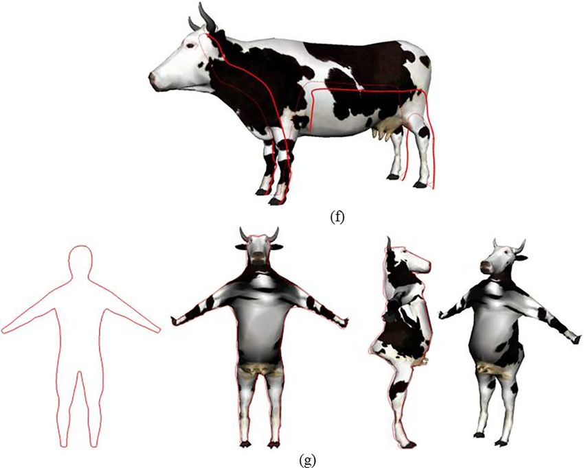
Multimedia Tools and Applications

deep regression network for inferring 3D face models from 2D sketches which fuses the
convolutional neural network and shape based features of the input sketch, Han et al. propose a
deep learning based sketching system for 3D face and caricature modelling which has a labor-
efficient sketching interface and supports gesture based interactions for users to further
manipulate initial face models [16]. By training a convolution neural network on a large
dataset generated by rendering sketches of various 3D shapes, incorporating the convolution
neural network into the sketch processing workflow to infer the depth and normal maps
representing a surface, introducing an intermediate convolution neural network layer to model
the dense curvature direction or flow field of the surface, and producing an additional output
confidence map along with depth and normal, Li et al. developed a method to create generic
freeform 3D surfaces from sparse, expressive 2D sketches [24]. By introducing a novel sketch
metaphor to create Poisson’s equation-based freeform surfaces, implementing a convenient
and flexible user interface, and using sparse strokes to achieve rapid modeling, Liu et al.
presented a new approach to create 3D models with rich details [26]. In order to offer a rich
source of information for a variety of computer-aided design tasks, Gryaditskaya et al. build a
database of product design sketches called OpenSketch [13]. It contains more than 400
sketches representing 12 man-made objects drawn by 7 to 15 product designers of varying
expertise and registers each sketch to its reference 3D model by annotating sparse correspon-
dences. In order to learn priors from data, Smirnov et al. present a deep learning-based system
for man-made shapes to infer a deformable parametric template model composed of Coons
surface patches and introduce a synthetic sketch augmentation pipeline and a loss function for
outputting non-self-intersecting shapes [35]. Through exploiting variational autoencoders to
learn the mapping between a simple 2D stick figure sketch and the output 3D model and the
embedding space around the model, Akman et al. propose the first method to create a 3D
human models from a single sketched stick fig. [1].
    Our proposed sketch-guided global modeling approach generates three different levels of
3D models directly from three different levels of profile curves. An initial model with circular
cross-section curves is created from the primary profile curves. It is changed into an interme-
diate model by deforming the initial model to fit the secondary profile curves represented with
elliptic cross-section curves. The final detailed model is obtained by fitting user-drawn key
cross-section profile curves which deforms the intermediate model to change the elliptic cross-
section curves into the user-drawn real key cross-section profile curves.

2.2 Template-based modeling

Template-based modeling includes generating a 3D template model and deforming the
template model to match user-drawn sketches.
    A main method of generating 3D template models is sketch-based shape retrieval. Various
sketch-based shape retrieval methods have been reviewed in [23]. According to [23], existing
sketch-based 3D model retrieval techniques can be categorized into: local 2D features versus
global 2D features, bag-of-words framework versus direct shape feature matching, fixed views
versus clustered views, and with view selection versus without view selection.
    Most of recent methods involve machine learning. Through learning structural groups from
a large database of scenes, Xu et al. developed a framework to automatically obtain seman-
tically valid and well-arranged scenes of 3D models from a freehand sketch drawing which
infers multiple scene objects [38]. Based on a novel data structure for fast retrieval of partial
matches, Guo et al. investigated an on-demand part extraction algorithm called CustomCut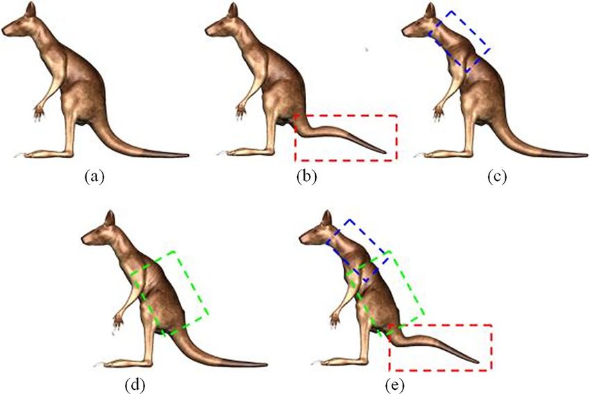
Multimedia Tools and Applications

[14]. For a user’s input sketch query, it searches a database to find partially matching shapes,
and identifies and extracts the region optimally matching the query in each shape to produce a
customized part. Sketch-based shape retrieval for procedural modelling was also investigated
in [17]. With the approach developed in the paper, user’s hand-drawn 2D sketches are mapped
to procedural model parameters through training a deep convolutional neural network by large
amounts of automatically generated synthetic line drawings. These procedural model param-
eters are used to generate multiple, detailed output shapes that resemble the user’s input
sketches. In order to take advantage of both global and local features, Li et al. proposed a
composite feature-based method to combine global features with local features which are
extracted from representative 2D views of 3D models [25]. The global feature is used to select
more relevant candidate models to the query sketch and the local feature is used to refine the
selected candidate models. In [44], a framework is proposed to extract a sketch-based local
binary pattern feature, determine the best view of a shape based on multilayer perceptrons
(MLPs), project 3D models into many multiview images, use transfer learning to obtain the
relationship between view images and sketches, and achieve shape retrieval based on two
Siamese MLP networks. In [45], a deep learning technique is developed for sketch-based
shape retrieval. The technique uses a sketch augmentation method to avoid simple image
transformation and more closely mimic human sketches, introduces a convolutional neural
network to learn the best viewing positions that best depict a 3D shape, and employs two
Siamese convolutional neural networks to develop a cross-domain learning strategy that pairs
up sketches and the 2D shape images. In [27], a framework is proposed to retrieve 3D models
from a user provided free-hand sketch. In order to obtain plausible shapes contained in a
sketch, a collection of shapes in the same category is used to train a shape space, and two
different intuitive editing modes based on the shape space are implemented into a user
interface for shape editing.
    After using one of the above methods to obtain a suitable 3D template model, a new 3D
model can be generated by deforming the template model to match user-drawn sketches. The
main work on this topic uses user-drawn silhouette in a single view as a deformation constraint
to deform the 3D template model such as in [22] which aligns user-drawn contour and a
template 3D model, determines the optimal correspondences between the contour and the
vertices on the template model, and uses the mean value coordinates to deform the 3D template
model to match the user-drawn contour. In [21], a new approach is proposed which combines
skeleton-based deformation with mesh editing to deform a 3D template model to fit user’s
drawn silhouette in a single view more efficiently.
    The approach proposed in this paper differs from the work given in [21, 22]. Apart from
deforming a template 3D model to match the primary profile curves in a single view, it adds
the secondary profile curves and key cross-section profile curves to further deform the model
to match all user-drawn profile curves in three orthographic views. Such an approach can
create more detailed and realistic 3D models.

2.3 Physics and PDE based deformations

Physics-based deformations have been introduced into computer graphics about three decades
ago. According to the comprehensive survey of various physically based deformable models
used in computer graphics, most significant methods include: finite element/difference/volume
methods, mass-spring systems, meshfree methods, coupled particle systems and reduced
deformable models based on modal analysis [31].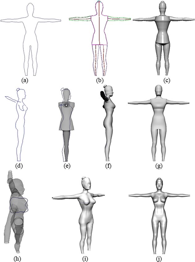
Multimedia Tools and Applications

    Recently, some new methods were introduced into computer graphics. For example, a finite
element method based on an elasto-plastic material model was implemented in [30], projective
dynamics was developed in [8], a co-rotated linear finite element method was employed to
handle large deformations of soft objects in [37], an example-based plasticity model based on
linear blend skinning was proposed in [20], and a boundary element based method was
investigated in [15] for fast simulation of brittle fracture. All these physics-based deformation
methods involve heavy numerical calculations.
    Partial differential equations (PDEs) have been widely used to describe various
physical phenomena. Geometric modeling and shape deformations using PDEs can be
regarded as physics-based and obtained by solving a vector-valued partial differential
equation subjected to a set of additional constraints called the boundary conditions.
Such a problem is a boundary value problem. Many methods have been developed to
solve various boundary value problems. By using a continuous genetic algorithm,
Arqub and Abo-Hammour present an efficient solver to solve systems of second-order
boundary value problems [3]. The finite difference approximation is used to represent
the derivatives of the differential equations in the systems, and the total residue of all
nodes in the systems of second-order boundary value problems is formulated. The
total residue is minimized, or the fitness function is maximized to obtain the solution
to the systems. Based on the assumption of strongly generalized differentiability and
the reproducing kernel theory, Arqub et al. investigate an iterative technique to obtain
the analytic and approximate solutions of second-order, two-point fuzzy boundary
value problems [4]. Through constructing the orthogonal basis from the obtained
kernel functions where the constraint initial condition is satisfied, Arqub develop
exact and numerical solutions to fuzzy Fredholm–Volterra integrodifferential equations
with the reproducing kernel Hilbert space method [2]. By applying the theory of
functional connections to embed the differential equation constraints into a constrained
expression containing a free-function which is a linear combination of orthogonal
basis functions with unknown coefficients and using linear/nonlinear least-squares to
determine the unknown coefficients, Johnston et al. obtain the solutions to eighth-
order boundary-value problems [19].
    Different from existing physics-based deformation methods involving heavy numer-
ical calculations, analytical solutions of PDE-based geometric modelling and shape
deformations may be obtainable and have been used in creation of surface [43] and
solid [42] models and surface blending [41]. They are much more efficient and simpler
to implement than numerical PDE-based approaches [6, 7, 36]. These analytical solutions
of PDEs are subjected to the constraints at two separate boundaries (2-sided patches)
[40]. However, many shape deformations are within the regions encircled by a single
closed boundary curve which can be divided into 4 boundaries (4-sided patches). How to
develop analytical solutions of PDE-based shape deformations for 4-sided patches has
not been solved. In this paper, we will tackle this problem.
    In what follows, the mathematical model consisting of PDE surfaces and generalized
elliptic curve-based interpolation surfaces is investigated in Section 3. Global modeling
consisting of sketch-guided global modeling and template-based global modeling is
proposed in Section 4 to generate a whole 3D character model quickly. Local modeling
techniques are presented in Section 5 to create local 3D details, and experiments are
made in Section 6. Finally, conclusions, limitations, and future work are discussed in
Section 7.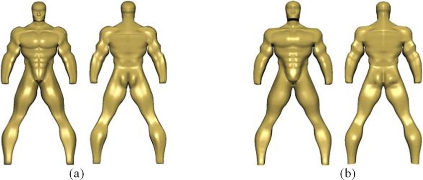
Multimedia Tools and Applications

3 Mathematical model

The mathematical model discussed below involves the descriptions of PDE surfaces consisting
of deformations caused by sculpting forces and interpolation surfaces which interpolate key
cross-section profile curves.

3.1 Deformation surfaces

The deformation surfaces are defined by an analytical solution developed below. Inspired by
the governing PDE for the elastic bending of thin plates, we use the fourth order partial
differential equations to determine the deformation surfaces, which are given below

                               ∂4        ∂4     ∂4
                           at1 4 þ at2 2 2 þ at3 4 t ðu; vÞ ¼ Pt ðu; vÞ                     ð1Þ
                              ∂u       ∂u ∂v    ∂v
                         ðt ¼ x; y; zÞ

where u and v are the parametric variables of the surface, x, y, and z are the position
components of the surface, at1, at2 and at3 are shape parameters, t(u, v)is a position function
whose components are x(u, v), y(u, v) and z(u, v), and Pt(u, v) is a sculpting force function
whose components are Px(u, v), Py(u, v), and Pz(u, v).
    When exact closed form solutions to PDE (1) are sought, different combinations of
the shape parameters at1, at2 and at3 lead to different closed form solutions. When
using PDE (1) to determine deformation surfaces, the values of the shape parameters
at1, at2 and at3 must be specified and the combination determined by the specified
values of the shape parameters at1, at2 and at3 is unique. Accordingly, the closed form
solution is unique whose unknown constants are uniquely determined by the boundary
conditions discussed below.
    Compared to the control point and surface point based shape manipulations, physics-based
approaches manipulate surfaces by applying virtual sculpting forces to deform the surfaces.
Since sculpting forces can be applied at any positions and in different ways, surface manip-
ulation using sculpting forces is physically meaningful and offers flexibility.
    Our deformation technique considers three important aspects: fast generation of deforma-
tion surfaces based on an approximate analytical solution, flexibility in specifying deformation
regions with any complicated shapes and with various sculpting forces, and an easy to use
interface for applying sculpting forces.
    Many parts of a virtual character, such as arms, legs and torso, are closed in one
parametric direction v, and open in the other direction u. When considering surface
deformations in the whole range of v parametric direction, the boundaries in v = 0 and
v = 1 are coincident and no boundary constraints are required. However, when discussing
the surface deformations in a local range of v parametric direction, the boundaries in v =
0 and v = 1 are two different ones and the boundary constraints must be satisfied. Due to
this reason, the analytical resolution of PDE (1) requires surface deformations to be
divided into two different types to respectively tackle 2-sided patches with u = 0 and u =
1 boundaries and 4-sided patches with u = 0, u = 1, v = 0, and v = 1 boundaries. For the
first type, it can change in a whole or local range in u direction but only covers a whole
range in v direction. For the second type, it can change within a local range in v direction
and keeps the ranges in u direction unchanged.
Multimedia Tools and Applications

   Once a deformation region has been specified, it is re-parameterized in a local coordinate
system. For simplifying mathematical symbols, we still use u and v to denote the parametric
variables in a local coordinate system below.
   We consider three types of sculpting forces: concentrated sculpting forces, line distribution
sculpting forces, and area distribution sculpting forces.
   The vector-valued concentrated sculpting force P(u, v) has three components px, py and pz,
and acts at any position (up0, vp0) where we use the subscript p to indicate sculpting forces.
   Since a line distribution sculpting force acting in any direction in a global coordinate system
can always be transformed into that acting in a parametric direction of a local coordinate
system, we here consider the line distribution sculpting force acting within a range {up0 ≤ u ≤
up1, v = vp0} in u parametric direction of a local coordinate system and taking a sine form below

                              Pt ðu; vÞ ¼ pt sin π u−up0 = up1 −up0                             ð2Þ

where t = x, y, z, and the sculpting force function Pt(u, v) reaches the maximum value pt at the
position {u = (up1 − up0)/2, v = vp0}.
   Similarly, if an area distribution sculpting force acts within a region {up0 ≤ u ≤ up1, vp0 ≤ v ≤ vp1}
and takes a sine form in both parametric directions, it can be described with the following equation

                  Pt ðu; vÞ ¼ pt sin π u−up0 sin π v−vp0 = up1 −up0 vp1 −vp0                          ð3Þ

where the sculpting force function Pt(u, v) reaches the maximum value pt at the position {u = (up1 −
up0)/2, v = (vp1 − vp0)/2}.
   For the first type of deformations, we transform the three types of sculpting forces into a
unified mathematical representation below

                             M                   N                 ¼
                                                                                    i
                 Pt ðu; vÞ ¼ ∑ sin mπu ptm þ ∑ ptmn cos2nπv þ p tmn sin2nπvÞ                     ð4Þ
                            m¼1                  n¼1

where M is the total terms of the sine series of the parametric variable u, and N is the total terms
of the Fourier series of the parametric variable v.
   The unknown constants ptm, ptmn and ptmn for concentrated sculpting forces, and line and
area distribution sculpting forces are given in Appendix A.
   For the first type of surface deformations, the deformation boundaries are at u = 0 and u = 1.
The positional and tangential continuity conditions at these two boundaries require
                                                             ∂t
                                  u¼0          t¼0              ¼0
                                                             ∂u                                       ð5Þ
                                                             ∂t
                                  u¼1          t¼0              ¼0
                                                             ∂u
where (t = x, y, z).
   The solution corresponding to sculpting force (4) and boundary conditions (5) represents a
deformation surface which has the following form

                tðu; vÞ ¼ Gt0 ðvÞ þ uGt1 ðvÞ þ u2 Gt2 ðvÞ þ u3 Gt3 ðvÞ
                           M                    N                    ¼                               ð6Þ
                         þ ∑ sinmπu ctm þ ∑ ctmn cos2nπv þ c tmn sin2nπvÞ
                            m¼1                  n¼1

where Gti(v) (t = x, y, z; i = 0, 1, 2, 3) are unknown functions, and ctm, ctmn and ctmn are un-
known constants.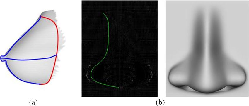
Multimedia Tools and Applications

  Inserting Eq. (6) into boundary conditions (5) and solving for the four unknown functions,
we obtain
                                 M
                    tðu; vÞ ¼ ∑    πm − u−3u2 þ 2u3 þ ½1−ð−1Þm u2 ðu−1Þ
                              m¼1                                                                             ð7Þ
                                            N              ¼
                                                                           i
                             þsinmπug ctm þ ∑ ctmn cos2nπv þ c tmn sin2nπvÞ
                                                    n¼1
Substituting Eq. (7) into PDE (1) and minimizing the error of the PDE, the unknown constants
ctm, ctmn and ctmn are found to be

                                     ctm ¼ ptm = π4 m4 at1
                                           ctmn ¼ −ptmn =f tmn                                                 ð8Þ
                                           ¼        ¼
                                           c tmn ¼ −p tmn =f tmn
where

                                 f tmn ¼ π4 4m2 n2 at2 þ π2 n2 at3 =3
                                         4                                                                  ð9Þ
                                       − m at1 þ 4m2 n2 at2 þ 16n4 at3

In Fig. 1, we depict the shapes of a PDE surface from the first type of surface deformations
caused by three different types of sculpting forces.
   For the second type of deformations, since surfaces in the v direction are non-closed, new
boundary conditions given below should be added to Eq. (5) to maintain positional and
tangential continuities at the four boundaries of the surfaces

Fig. 1 First type of deformations. a Original model. b A concentrated sculpting force acts at the tail. c A line
distribution force acts at the neck. d An area distribution force acts at the back. e Combination of deformations in
(b), (c) and (d)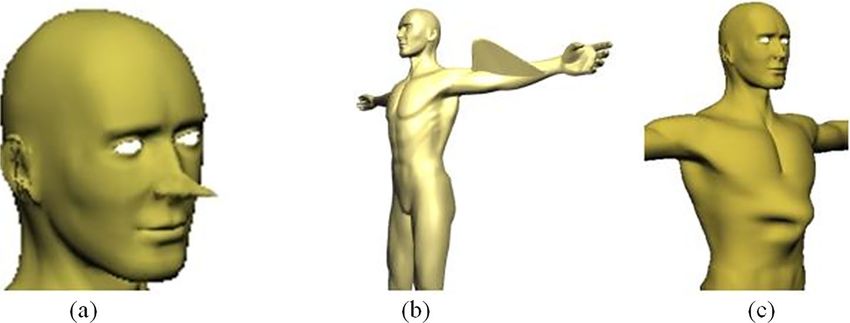
Multimedia Tools and Applications

                                                                   ∂t
                                     v¼0            t¼0               ¼0
                                                                   ∂v                                       ð10Þ
                                                                   ∂t
                                     v¼1            t¼0               ¼0
                                                                   ∂v
where t = x, y, z.
   In order to construct position functions which meet boundary conditions (5) and (10), we
rewrite the three types of sculpting forces into the following form
                                                M   N
                                 Pt ðu; vÞ ¼ ∑ ∑ ptmn sin mπu sin nπv                                       ð11Þ
                                              m¼1 n¼1

where t = x, y, z, M is the total terms of the sine series of the parametric variable u, and N is the
total terms of the sine series of the parametric variable v.
   The unknown constants ptmn for concentrated sculpting forces, and line and area distribution
sculpting forces are given in Appendix B.
   The solution which satisfies boundary conditions (5) and (10) exactly can be taken to be

                       tðu; vÞ ¼ vð1−vÞ Gt0 ðvÞ þ uGt1 ðvÞ þ u2 Gt2 ðvÞ

                                                 M N                                            ð12Þ
                                þ u Gt3 ðvÞ þ ∑ ∑ d tmn sin mπu sin nπv
                                     3
                                                    m¼1 n¼1

where Gt0(v), Gt1(v), Gt2(v) and Gt3(v) are the unknown functions, and dtmn are unknown
constants.
   Substituting Eq. (12) into boundary conditions (5) and (10), we obtain
                                               M    N
                         t ðu; vÞ ¼ vð1−vÞ ∑ ∑ fπmf−u þ ½2 þ ð−1Þm  u2
                                              m¼1 n¼1                                                       ð13Þ
                                 −½1 þ ð−1Þm  u3 þ sin mπu d tmn sin nπv

Introducing Eq. (13) into PDE (1) and minimizing the error of the PDE, we obtain
dtmn below

                             d tmn ¼ n2 ptmn = mπ2 d tmn                   ð14Þ

Fig. 2 Second type of deformations. a Nose deformation in a small region caused by a concentrated sculpting force.
b Arm deformation in a very narrow curved band region caused by a line distribution sculpting force. c Chest
deformation in a local region with an irregular boundary shape caused by an area distribution sculpting force
Multimedia Tools and Applications
where
d tmn ¼ 2m3 at1 þ 6n4 −mπ2 =12 þ 1=m at3 ð15Þ
In Fig. 2, we demonstrate shape changes in different deformation regions of a PDE surface
from the second type of deformations caused by concentrated sculpting forces, and line and
area distribution sculpting forces. With our proposed approach, these deformed shapes were
created easily and quickly.
3.2 Interpolation surfaces
Interpolation surfaces can be regarded as a special case of PDE surfaces where the sculpting
forces used to create deformation surfaces are zeroed.
Unlike the existing work of reconstructing surfaces from sampled planar cross-sections of
arbitrary orientation [5] and non-parallel cross-section curves with genus-1 constraint [47], the
interpolation surfaces introduced below are based on generalized elliptic curves and construct-
ed from boundary curves and boundary tangents together with in-between key cross-section
profile curves.
Key cross-section profile curves are the framework of an interpolation surface. In
order to describe key cross-section profile curves with a unified mathematical represen-
tation, we introduce the conception of generalized elliptic curves which are defined by
the following equation
J
x ¼ x0 þ ∑ x2 j−1 cos 2 jπv þ x2 j sin 2jπv
j¼1
J ð16Þ
y ¼ y0 þ ∑ y2 j−1 sin 2jπv þ y2 j cos 2jπv
j¼1
z ¼ zc
where J is the total terms of the cosine series and sine series, respectively, zc is the
coordinate value of the key cross-section profile curve in zdirection, and xk and yk
(k = 0, 1, 2, 3, ⋯, 2J) are unknown constants which can be determined by least squares
curve fitting.
In Fig. 3, we make a comparison among the original key cross-section profile curves,
corresponding generalized elliptic curves and standard ellipses where the curves in red, green
and blue are the original ones, produced using our approach, and created with the standard
ellipses, respectively. From the figure, big differences can be observed between the original
J=2 J=3 J=4
Fig. 3 Comparison among original key cross-section profile curves (red), generalized elliptic curves (green), and
standard ellipses (blue)Multimedia Tools and Applications
Fig. 4 Generalized elliptic curve-based interpolation surface. a Original model. b 150 GECs. c 240 GECs
ones and standard ellipses. In contrast, with small values of J, generalized elliptic curves
approach the original curves very accurately. It indicates that generalized elliptic curves can
represent key cross-section profile curves with high accuracy.
In Fig. 4, we give a dog model represented by interpolation surfaces with different numbers
of generalized elliptic curves. It can be observed from the images in the figure that using a
small number of generalized elliptic curves, we can obtain the interpolation surfaces which fit
the original dog model very well. With the increase of generalized elliptic curves, the
interpolation surfaces improve its modeling accuracy quickly.
4 Global modeling
Global modeling is the first stage of a modeling process. It is to create a whole model for
further modifications to be made with local modeling.
For global modeling, we present two different modeling approaches: sketch-guided model-
ing and template-based modeling. With the former, the animator/modeler sketches the primary,
secondary, and key cross-section profile curves of a 3D model, and the system creates the 3D
model from these profile curves automatically. There is no need to refer to any existing
models, and the animator has a total freedom to create the characters which they design.
Therefore, it is especially suitable for the creation of grotesque characters such as monsters.
With the latter, the primary, secondary, and key cross-section profile curves of a character are
compared to those of a template model from a model database. This approach can create a
detailed global model more efficiently and is more suitable for modeling of common charac-
ters. However, it requires a template model.
According to the above discussions, we can identify the following differences between
sketch-guided global modeling and template-based global modeling.
1) Different global modeling process: Sketch-guided global modeling creates a new 3D
character model directly from user’s drawn sketches. However, template-based global
modeling creates a new 3D character model by deforming a template character model to
fit user’s drawn sketches.
2) Different details: Sketch-guided global modeling can create rough models only since a
single sketch in one view plane or several sketches in different view planes are not enough
to define a 3D model with good details. In contrast, template-based global modeling
makes use of good details of a template model and solves the problem that sketch-guided
global modeling can create rough models only.Multimedia Tools and Applications
3) Different flexibilities: Sketch-guided global modeling is more flexible in creating rough
3D shapes which users want. By comparison, template-based global modelling cannot
create some special 3D models such as grotesque character models whose template
models are not available.
4.1 Sketch-guided global modeling
Sketch-guided global modeling is undertaken through three different stages of modeling with
an increasing level of details at each stage. As shown in Fig. 5 and the accompanied video, the
first stage creates an initial global model from the primary profile curves; the second stage
creates an intermediate global model with the secondary profile curves; and at the third stage,
the final global model is refined with key cross-section profile curves.
Here the primary profile curves are the silhouette curves which are the most suitable for
describing the whole shape of a 3D model. An intermediate global model is obtained by
adding the constraints of secondary profile curves to the initial global model. The secondary
profile curves are also some silhouette curves of a 3D model and its parts but viewed from the
perpendicular directions to the first one. For 3D models with a complicated geometric shape,
some of their parts can be removed to simplify the model, and the primary and secondary
profile curves are produced from the simplified model. For the removed parts, their initial and
intermediate global models are created from their own primary and secondary profile curves. A
final global model is produced by modifying the key cross-section profile curves which are
perpendicular to the primary and secondary profile curves and add the features which have not
been characterized by the primary and secondary profile curves.
4.1.1 Initial global models
In order to create an initial global model, we sketch primary profile curves. For the modeling
of a female character, we firstly sketch a primary profile curve as shown in Fig. 6a. Next, we
identify the boundary curves which segment the female profile curve into different regions i.e.,
hair, arms, legs and torso, and determine the central curves between two profile curves of a
region (Fig. 6b). The key cross-sections are then automatically located according to the variety
of the curvature along the two profile curves, which can be manually edited if necessary. We
Fig. 5 Our proposed sketch-guided modeling quickly creates an initial global model from a profile curve in (a),
uses a secondary profile curve in (b) to generate an improved intermediate global model in (c), and introduces
key cross-section profile sketches in (d) to obtain a fine detailed global model in (e)Multimedia Tools and Applications Fig. 6 Sketch-guided global modeling. a Primary profile curve. b Segmentation of primary profile curves and central curves. c Initial global model. d Secondary profile curves. (e) Secondary profile curves are applied on the initial global model. f, g Intermediate global model. h One key cross-section profile curve of the female is applied on the intermediate global model. i Breast of the female is created from the key cross-section profile curve. j Final global model is obtained by introducing more key cross-section profile curves take circles to be the first approximation to the cross-section curves of the parts of the female model in these key cross-sections whose centers are situated on the central curves and
Multimedia Tools and Applications
diameters are determined by the distance between two profile curves of the parts. Then, the
initial global model of each part is created and represented with a surface which interpolates
these circles.
For the joints between legs, torso, and arms, the boundary curves between two adjacent
parts are determined. Then, the tangents of surfaces at these two boundary curves are
calculated. Finally, we create a smooth transition surface between these two boundary curves
according to the information of the boundary curves and tangents at the boundary curves to
smoothly connect the arm and leg surfaces to the torso surface. The image in Fig. 6c is a
generated initial global model.
4.1.2 Intermediate global models
After an initial global model is obtained, the secondary profile curves shown in Fig. 6d are
applied on the initial global model as indicated in Fig. 6e. Then, new positions of key cross-
sections, represented with ellipses, are obtained automatically according to the variety of the
curvature along the primary and secondary profile curves. Once again, manual edit of the
position of key cross-sections is allowed. Finally, the semi-major and semi-minor axes of the
ellipses are calculated from the primary and secondary profile curves, and a new 3D model is
created by interpolating these key cross-section ellipses.
The transition surfaces between different parts produced in the first stage are regenerated
according to the boundary curves and tangents of the adjacent parts. The image in Fig. 6f and g
indicates a generated intermediate global model.
4.1.3 Final global models
The cross-section contours obtained from the intermediate global models are standard ellipses.
However, the real cross-section contours of 3D organic models are irregular curves which
contain shape features of the models. In order to add these features to the intermediate global
models, we sketch new contours at the positions of the key cross-sections or modify the
existing contours of the character models in these key cross-sections. In this way, the ellipses at
these key cross-sections are changed into the real cross-section profile curves. We use
generalized elliptic curves to represent these real key cross-section profile curves. The final
global models are produced and represented with PDE surfaces which interpolate these
generalized elliptic curves and provide a powerful means for further local modeling.
Figure 6h demonstrates that although only one key cross-section profile curve of the female
breast is applied on the intermediate global model, excellent approximation of the female
breast is obtained as shown by Fig. 6i.
By creating or modifying more key cross-section profiles, the final detailed global model is
created and depicted in Fig. 6j.
A possible extension to the above treatment is that the secondary and key cross-section
profile curves can be taken in arbitrary planes and directions.
4.2 Template-based global modeling
Template-based global modeling is to use the corresponding relationships between sketched
profile curves and those of a template model with a similar topology to transform the template
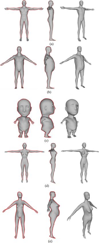
model into a new one represented with PDE surfaces which fits all the sketched profile curves.Multimedia Tools and Applications Fig. 7 Different character models built from template-based global modeling. An existing male model in (a) is b changed into a fatter one in (b) and a boy in (c). An existing female model in (d) is changed into a pregnant woman in (e). An existing cow model in (f) is changed into a new model in (g). Among each group of the created 3D models, the left is from the primary profile curve, the middle is from the secondary profile curve, and the right is from the key cross section profile curves. The red primary profile of a male in (g) is used to change the cow model (f) into the right 3D model in (g) Character models have complicated shapes, which cannot be completely and accurately defined with a 2D character sketch or some 2D character sketches in different view planes. A template character model has all the components and details of this type of character models. Template- based global modeling creates a whole 3D character model by deforming a template character model to match user’s drawn sketches. It has the property of making use of the components and details of the template character model, and the shape defined by the user’s drawn sketches. Similar to sketch-guided global modeling, Template-based global modeling can also be classified into three different global models: low-level global models, medium-level global models, and high-level global models which correspond to the model from the primary profile, primary and secondary profiles, and primary and secondary profiles plus key cross-section profile curves, respectively. The process of template-based global modeling is shown in the accompanied video and explained below. 4.2.1 Low-level global modeling For low-level global modeling, we firstly sketch primary profile curves of a virtual character. With the method of shape matching and retrieval proposed in [11], we search a database to find a template model which has the primary profile curves fitting the sketched ones best. Through geometrical transformations, the primary profile curves of the template model align with the sketched ones. Then, the radial basis function (RBF) interpola- tion is applied to deform the template model into a low-level model whose profile curves fit the sketched ones exactly. The images in Fig. 7b and c demonstrate how a male in Fig. 7a is changed into a fatter one and a boy. Those in Fig. 7e demonstrate how a female in Fig. 7d becomes a pregnant woman. And the images in Fig. 7g show the evolution of a cow in Fig. 7f to a different one. Among the created 3D models, those on the left are from primary profile curves. 4.2.2 Medium-level global modeling For medium-level global modeling, secondary profile curves of the low-level model and its parts are first obtained. For the secondary profile curves to be modified, the corresponding new secondary profile curves are generated. By applying the geometric transformation operations and RBF interpolation which make the secondary profile curves of the low-level model and its parts fit the generated ones, the low-level model is changed into a medium-level model whose primary and secondary profile curves are the same as the generated ones. The medium-level 3D models from the medium-level global modeling are shown in the middle of Fig. 7b, c, e and g. 4.2.3 High-level global modeling For high-level global modeling, we first decide the positions of the key cross-sections where the shape features of a virtual character at these key cross-sections have not been
Multimedia Tools and Applications
Multimedia Tools and Applications

Fig. 7 (continued)

characterized by the medium-level model from the first two stages of the global model-
ing. Then, the key cross-section profile curves of the medium-level model are displayed
and modified or new cross-section curves are created. Finally, RBF interpolation is
employed to create new surface shapes which exactly fit all primary, secondary, and
modified or new created key cross-section profile curves, and generate high-level global
models. The created 3D models on the right of Fig. 7b, c, e and g are from high-level
global modeling.
   In the above, we use key cross section curves to create final global models and high-level
global models. In fact, such a method can be extended to arbitrary spatial characteristic curves.
That is to say, we can create final and high-level global models by making sketched spatial
characteristic curves fit those of an existing model. For this extension, z component in eq. (16)
takes the form of trigonometric series to describe arbitrary spatial characteristic curves.

5 Local modeling

Local modeling is to create regional models or change local shapes to add 3D details. In
addition to the existing shape manipulation approaches, we investigate four shape manipula-
tion techniques. They include: shape manipulation by PDE surfaces, generalized elliptic
curves, sketch-guided deformations, and template-based shape changes.
Multimedia Tools and Applications

5.1 PDE based shape manipulation (PDESM)

With our PDE based technique, three methods can change the shape of a surface. They are
sculpting forces, shape parameters, and boundary curves and boundary tangents. Among these
methods, sculpting forces are the most powerful and flexible in shape manipulation as
introduced in Subsection 3.1 and shown by Figs. 1 and 2. Compared to the control point or
surface point based shape manipulations, the sculpting force based shape manipulation has the
following advantages:

(1) A sculpting force can be specified at any positions conveniently. In contrast, the shape
    manipulation operations of the control point or surface point based approach cannot be
    performed at the positions where no surface or control points exist.
(2) Deformation regions with any complicated boundary shapes can be easily specified with
    the sculpting force based shape manipulation. Oppositely, the control point and surface
    point based approaches are difficult to control a shape change which occurs within a pre-
    specified region with a complex boundary. Such a function is very useful for some
    surface deformations. For example, if we want to model a human nose, the deformation
    should occur only within the boundary curve between the nose and the face which has an
    irregular geometric shape.
(3) Sculpting force based approach is very powerful in both global and local shape
    manipulations.

Apart from sculpting forces, shape parameters, boundary curves, and boundary tangents are
also effective in shape manipulations as demonstrated below.
   When non-zero boundary curves and tangents are to be considered, boundary conditions
and the solutions of PDE (1) should be modified accordingly. Due to the limitation of space,
we will not discuss this here.
   By changing shape parameters, we can obtain different deformation shapes as depicted by
Fig. 8b and c. Figure 8d and e give an example how boundary curves and boundary tangents
affect surface shapes.

Fig. 8 PDE based surface manipulation of a pig torso. a Original model. b Deformation with shape parameters
1.0. c Deformation with shape parameters 0.3. d Shape variation by changing boundary curves. e Shape variation
by changing boundary tangents
Multimedia Tools and Applications
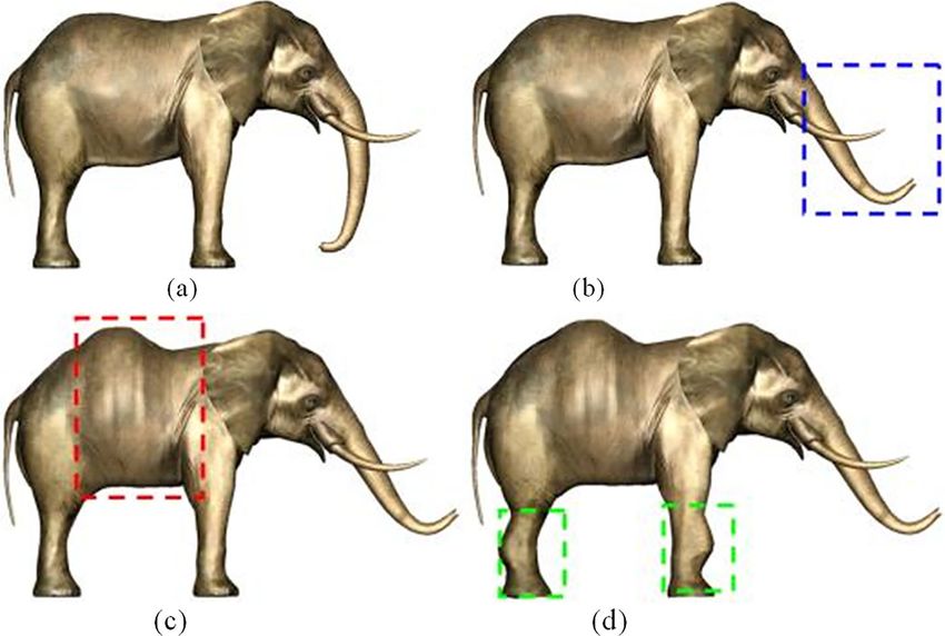
5.2 Generalized elliptic curves driven shape manipulation (GECDSM)
We can change the shape or size of generalized elliptic curves describing key cross-section
profile curves, or perform geometrical transformations to achieve new shapes.
As shown in Fig. 9, the geometric transformations are applied to the generalized
elliptic curves of the elephant trunk in Fig. 9a to change it into a new shape in Fig. 9b.
The size of the generalized elliptic curves of the elephant torso is changed to obtain the
torso shape shown in Fig. 9c. The local shapes of generalized elliptic curves of the
elephant legs are changed to generate new leg shapes depicted in Fig. 9d.
5.3 Sketch assisted shape manipulation (SASM)
For sketch assisted shape manipulation, we present two methods: sketch on a 3D model, and
auxiliary lines assisted sketches.
Sketch on a 3D model is to sketch a few local profile curves and generate a local model
from these profile curves. For example, in order to create a female breast, we sketch a closed
red curve on the chest of a female model and two blue profile curves of a woman breast on the
same model as shown in Fig. 10a.
Auxiliary lines assisted sketches are to add some supplemental sketches and provide
additional geometric information to define a local shape. For example, the profile curve of a
human gives the main contour of a nose. By increasing an auxiliary sketch curve in bright
green along the interface between the nose and face shown on the left of Fig. 10b, we create a
rough shape of a human nose shown on the right.
Fig. 9 Generalized elliptic curves driven shape manipulation. a Original model. b Deformation of the trunk by
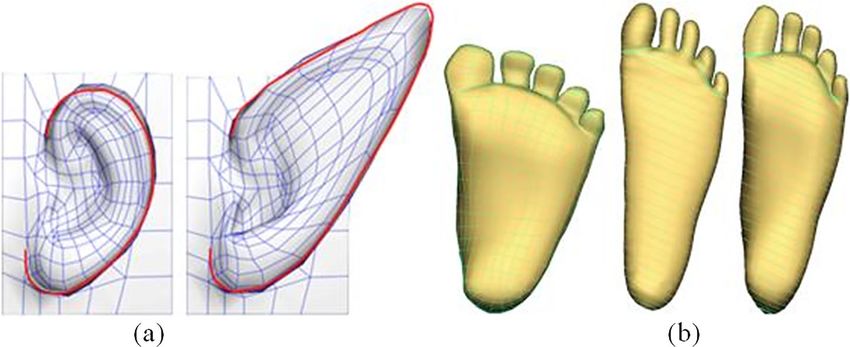
geometrical transformation. c Global deformation of the torso. d Local deformation of the legsMultimedia Tools and Applications Fig. 10 Sketch assisted shape manipulation. a A female breast from sketches on a 3D model. b A human nose created by adding an auxiliary sketch curve 5.4 Template-based shape manipulation (TBSM) Template-based shape manipulation includes local part creation through use of the correspond- ing relations between the created local profile curves and those of existing character parts and regional shape changes by comparing the created key cross-section curves to the correspond- ing ones of a template character model. In Fig. 11a, we draw the profile curve of an ear on the right, use the corresponding relation between the profile curve and that of a similar model in our database shown on the left, and change the existing ear on the left into a new one on the right. In Fig. 11b, we compare the cross section curves in the middle, which are ellipses created by the sketch-based global modeling, to those of a template foot model on the left and change the foot model originally represented with ellipses in the middle into a new model on the right which has real cross section curves of a human foot. Our proposed modeling system also represents a virtual character with both a PDE model and a polygon or NURBS model. With such a treatment, we can carry out shape manipulations on the PDE model with our proposed local modeling techniques, and do the work on the polygon or NURBS model using the existing local shape manipulation methods. Figure 12a and b indicate interrelated PDE and polygon representations of the same model. Fig. 11 Sketch-based shape manipulation. a Referring to an existing local part. b Referring to existing cross section curves
Multimedia Tools and Applications

Fig. 12 PDE and polygon representations of a same model. a Generalized elliptic curves and PDE surfaces. b
Polygon model with mesh

6 Experiments

Except for sketch-guided global modeling and template-based global modeling which were
implemented differently, all the mathematical equations developed in Section 3 and local
modeling techniques were implemented into two different versions. The first version uses
Microsoft Visual C++ and OpenGL. The Autodesk Maya provides a powerful platform in
drawing 3D sketches and quickly integrates PDE surface-based 3D models with polygon and
NURBS modeling. The second version uses the Maya Python scripts. Template-based global
modeling was implemented with Microsoft Visual C++ and OpenGL, and sketch-guided
global modeling was implemented using Maya Python scripts.
    With the implemented software, we carried out experimental work to compare our proposed
approach to the existing ones.
    Our first experiment is to examine the amount of information used to represent a same
character model. For a polygon model given in Fig. 13a, the total polygon faces are 9451 and
vertices are 6413. Using our proposed sketch-based PDE approach, we rebuilt the model
shown in Fig. 13c which consists of 32 PDE surfaces determined by a total of 139 generalized
elliptic curves shown in Fig. 13b and 2224 coefficients. This experiment indicates our
proposed approach requires much smaller data to represent a model, accordingly, greatly
reduces the data storage and the demand for computer resources.
    Our second experiment is to compare manual operations of shape manipulation with
the sculpting force-based method proposed in Subsection 3.1 and by the vertex-based

Fig. 13 Comparison of information amount used to represent a model. a Polygon model. b Generalized elliptic
curves. c PDE model
Multimedia Tools and Applications
Fig. 14 Comparison of shape manipulation between sculpting force-based method of PDE deformation surfaces
and vertex-based method of polygon models. (a) Undeformed shape. (b) Deformed shape achieved by sculpting
force-based shape manipulation. (c) Deformed shape achieved by vertex-based shape manipulation
method which tweaks the vertices of polygon models. With the deformation surfaces
proposed in Subsection 3.1, one manual operation was required to draw a closed curve
on the chest surface of the 3D model shown in Fig. 14(a), the implemented sculpting
force-based algorithm automatically parametrized the region enclosed by the drawn
closed curve into {0 ≤ u ≤ 1, 0 ≤ v ≤ 1}. After that, another manual operation was required
to move a mouse and the movement was automatically changed into a sculpting force to
create the chest deformation shown in Fig. 14(b). Since the chest deformation region has
an irregular boundary, when tweaking the vertices of the 3D polygon model in the same
deformation region, 15 manual operations were required to create a similar chest
deformation in a similar deformation region shown in Fig. 14(c). This example indicates
that the sculpting force-based shape manipulation proposed in this paper can greatly
reduce manual operations and raise modeling efficiency.
Our third experiment is to investigate the efficiency of building a character model using
different approaches. We ask an animator to build a same character model. He took about 10 h
to build the model in Fig. 15a using polygons, and about 7 h to create the same model in
Fig. 15 Comparison of efficiency of different modeling approaches. (a) Polygon modeling. (b) Sketch-based
PDE modelingYou can also read