Research of Personalized Recommendation Technology Based on Knowledge Graphs - MDPI
←
→
Page content transcription
If your browser does not render page correctly, please read the page content below
applied
              sciences
Article
Research of Personalized Recommendation Technology Based
on Knowledge Graphs
Xu Yang, Ziyi Huan, Yisong Zhai and Ting Lin *

                                          School of Computer Science and Technology, Beijing Institute of Technology, Beijing 100081, China;
                                          yangxu@tsinghua.edu.cn (X.Y.); 3220200891@bit.edu.cn (Z.H.); 3220180899@bit.edu.cn (Y.Z.)
                                          * Correspondence: linting@bit.edu.cn

                                          Abstract: Nowadays, personalized recommendation based on knowledge graphs has become a hot
                                          spot for researchers due to its good recommendation effect. In this paper, we researched personalized
                                          recommendation based on knowledge graphs. First of all, we study the knowledge graphs’ construc-
                                          tion method and complete the construction of the movie knowledge graphs. Furthermore, we use
                                          Neo4j graph database to store the movie data and vividly display it. Then, the classical translation
                                          model TransE algorithm in knowledge graph representation learning technology is studied in this
                                          paper, and we improved the algorithm through a cross-training method by using the information of
                                          the neighboring feature structures of the entities in the knowledge graph. Furthermore, the negative
                                          sampling process of TransE algorithm is improved. The experimental results show that the improved
                                          TransE model can more accurately vectorize entities and relations. Finally, this paper constructs a
                                          recommendation model by combining knowledge graphs with ranking learning and neural network.
                                          We propose the Bayesian personalized recommendation model based on knowledge graphs (KG-BPR)
                                          and the neural network recommendation model based on knowledge graphs(KG-NN). The semantic
                                information of entities and relations in knowledge graphs is embedded into vector space by using

                                          improved TransE method, and we compare the results. The item entity vectors containing external
Citation: Yang, X.; Huan, Z.; Zhai, Y.;   knowledge information are integrated into the BPR model and neural network, respectively, which
Lin, T. Research of Personalized
                                          make up for the lack of knowledge information of the item itself. Finally, the experimental analysis is
Recommendation Technology Based
                                          carried out on MovieLens-1M data set. The experimental results show that the two recommendation
on Knowledge Graphs. Appl. Sci.
                                          models proposed in this paper can effectively improve the accuracy, recall, F1 value and MAP value
2021, 11, 7104. https://doi.org/
                                          of recommendation.
10.3390/app11157104

Academic Editor: Diana Kalibatiene
                                          Keywords: knowledge graph; representation learning; personalized recommendation; Bayesian
                                          personalized ranking
Received: 17 June 2021
Accepted: 24 July 2021
Published: 31 July 2021
                                          1. Introduction
Publisher’s Note: MDPI stays neutral            With the widespread application of information technology, the information contained
with regard to jurisdictional claims in   in the network has grown rapidly, which has also brought about information overload
published maps and institutional affil-   and information confusion. Information overload makes the amount of information in
iations.
                                          the social media far greater than what it can carry. Information confusion often makes
                                          people unable to find useful data when searching information. Furthermore, it makes
                                          people attracted by irrelevant and messy data. How to reduce information overload and
                                          information confusion has also become a research hotspot. As a result, classification catalog,
Copyright: © 2021 by the authors.         search engine and recommendation system appear.
Licensee MDPI, Basel, Switzerland.              The earliest recommendation model is collaborative filtering algorithm, which mainly
This article is an open access article    discovers the content that the user is interested in through user behavior data, and rec-
distributed under the terms and           ommends it to the user [1]. Netflix is the first video website to adopt a collaborative
conditions of the Creative Commons
                                          filtering algorithm. According to users’ rating data of movies, Netflix mines users’ inter-
Attribution (CC BY) license (https://
                                          ests and recommends movies for users. Since then, the recommendation algorithm has
creativecommons.org/licenses/by/
                                          emerged. However, in the commercial recommendation system, such as video website
4.0/).

Appl. Sci. 2021, 11, 7104. https://doi.org/10.3390/app11157104                                                https://www.mdpi.com/journal/applsci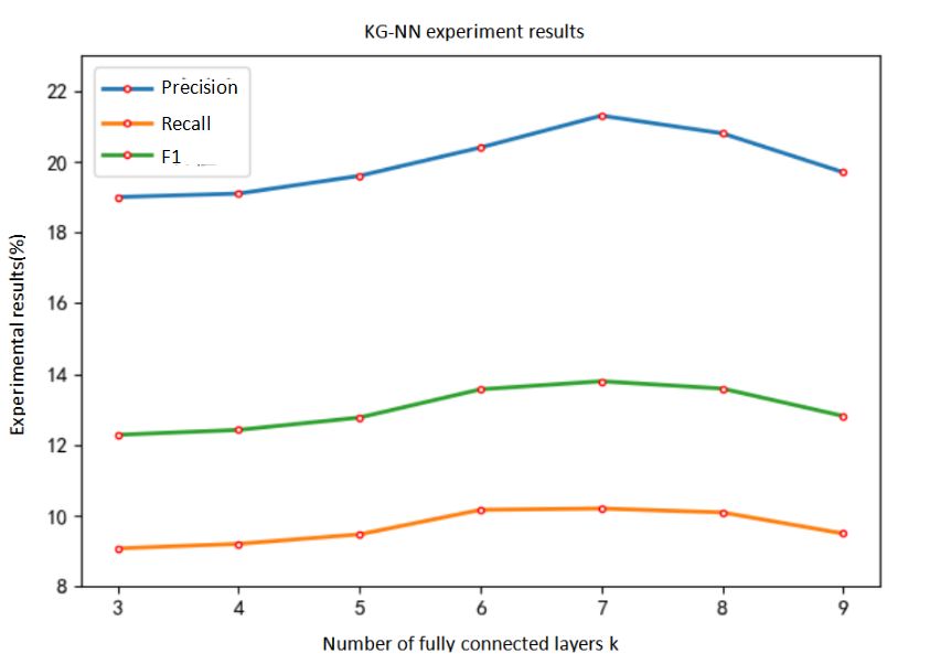
Appl. Sci. 2021, 11, 7104                                                                                          2 of 25

                            or e-commerce website, the scale of users and items is huge. Meanwhile the interaction
                            information between them is very limited. Therefore, the problem of data sparsity arises.
                                  The recommendation algorithm has been continuously improved, resulting in the
                            recommendation model based on neural network, such as DeepFM, Wide&Deep, etc. They
                            cannot only effectively improve the sparse problem of user item matrix in collaborative
                            filtering algorithm, but also can automatically combine features, greatly improving the
                            effect of recommendation [1]. At present, Tencent video, Taobao, TikTok and other websites
                            have been using neural networks to optimize their recommendation models, in order to
                            increase click-through rate and stay time to bring greater benefits.
                                  The purpose of knowledge graphs is to show entities, events and their relations in the
                            real world in a structured form, and to present Internet information in a way that people
                            can easily understand. Its essence is a knowledge base with a directed graph structure [2].
                            In order to improve the effect of recommendation, more and more researchers begin to
                            study the recommendation model based on knowledge graphs. This recommendation
                            method not only integrates the external rich semantic information of item entities, but also
                            introduces the association information between items, which can effectively alleviate the
                            problem of data sparsity and cold start [3]. At the same time, through the structural display
                            of knowledge graphs, various complex relations between projects can be displayed vividly.
                            Therefore, the hybrid recommendation model that introduces the knowledge graphs has
                            become a trend of current research [4].
                                  This paper works on the knowledge graphs of the movie field and constructs the
                            knowledge graphs. Furthermore, we mine the data of entities and their relations. We use
                            different methods to optimize the movie knowledge graphs. Furthermore, we improve
                            the knowledge graph representation learning method. Combined with Bayesian person-
                            alized recommendation and deep neural network, the movie recommendation model is
                            constructed. It provides a new solution for the application of knowledge graphs and the
                            recommendation model. The main contributions of this paper are as follows:
                            (1)   Improve the TransE [5] algorithm, which is a knowledge graph representation learning
                                  method, and propose a hybrid feature learning method based on the nearest neighbor
                                  feature information of entities in knowledge graphs. At the same time, we improve the
                                  negative sampling process. Experiments show that the proposed model can improve
                                  the effect of representation learning.
                            (2)   We proposed a movie recommendation algorithm KG-BPR that combines knowledge
                                  graphs and Bayesian personalized ranking. Two movie recommendation models
                                  based on knowledge graphs are proposed. The first method combines the knowledge
                                  graphs and Bayesian personalized ranking, introduces the movie entity vector matrix
                                  in ranking learning to help generate the user feature matrix and movie feature matrix
                                  in BPR ranking model. Furthermore, it applies them in the scoring prediction process.
                                  The advantages of this algorithm are verified by experiments.
                            (3)   A movie recommendation method KG-NN, which combines the knowledge graphs
                                  and deep neural network, is proposed. This method inputs the knowledge graphs
                                  data as auxiliary information into the neural network for recommendations. It makes
                                  up for the original model’s lack of consideration of the content information of the
                                  item itself and introduces related data external knowledge. Experiments show its
                                  advantages in movie recommendation.
                                 The rest of this paper is organized as follows: Section 2 briefly describes the related
                            work and research progress of knowledge graphs and recommendation systems. Section 3
                            elaborates the main process of constructing the knowledge graphs of movie, and shows
                            the constructed knowledge graphs with neo4j. Section 4 improves the TransE representa-
                            tion learning algorithm by using a method of hybrid feature learning method that uses
                            the nearest neighbor feature structure information of entities in the knowledge graphs.
                            Finally, two movie recommendation models, KG-BPR and KG-NN, are proposed. Section 5
                            describes the experimental process. We conduct experiments on the improved TransE
                            representation learning model and the proposed recommendation model. Furthermore, we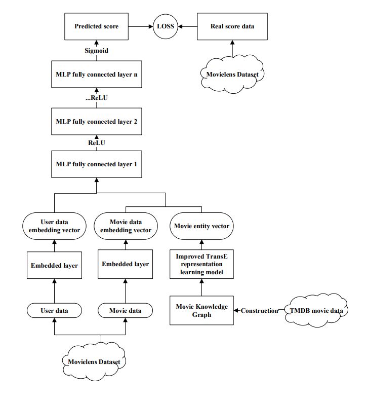
Appl. Sci. 2021, 11, 7104                                                                                          3 of 25

                            evaluate the effect of the model according to the evaluation method. Section 6 summarizes
                            the contribution of this paper, and proposes the improvement we can make in the future.

                            2. Related Works
                                  Knowledge graph: In the 1970s, expert systems appeared. They use knowledge
                            and reasoning processes to solve difficult and professional problems. This is the earliest
                            knowledge graph. Subsequently, with the continuous development of linked open data,
                            there are many knowledge acquisition methods based on information extraction technology,
                            such as open domain information extraction OIE and Nell [6].
                                  Google first put forward the concept of knowledge graphs in 2012, and applied
                            knowledge graphs in its search business in the same year, which achieved good results.
                            After that, Sogou in China also applied the knowledge graphs to its own search business.
                            At present, knowledge graphs are constantly applied in various fields, which has brought
                            far-reaching influence, such as Freebase, DBpedia, YAGO, etc. Recently, the knowledge
                            graphs of COVID-19 has been jointly constructed by NCBI, OpenKG and a number of
                            scientific research institutions in China. It has been made public to the world, which
                            provides great help for the global virus research and treatment [7].
                                  At present, the key technologies of knowledge graphs involve information retrieval,
                            data mining and natural language processing. In recent years, the methods are mainly di-
                            vided into knowledge driven and data driven. Knowledge driven combines the knowledge
                            and experience of experts to build knowledge systems in a specific field, and expands to
                            other open fields through accumulation. Data driven takes mathematical statistics as the
                            theoretical basis. It takes large-scale data as the driving force, and automatically obtains
                            relevant knowledge through machine learning, data mining and other technologies. The
                            construction of knowledge graphs is divided into several steps, which involve entities
                            recognition, relations extraction and attribute correction. Among them, the object of entity
                            recognition is to recognize entity information from text data. At present, there are three
                            main methods to complete the task, namely, rule-based method, machine learning method
                            and hybrid method. The purpose of relations extraction is to connect all entities and extract
                            their association information to form a complex knowledge network.
                                  In general, knowledge graphs contain a large amount of valuable information. Through
                            the organization and management of unstructured data, the value of data can be deeply
                            explored. Furthermore, the knowledge network can be vividly displayed by combining
                            machine learning algorithms. Therefore, more and more experts begin to do research on
                            knowledge graphs.
                                  Meanwhile, with the rapid development of machine learning, entity recognition based
                            on machine learning methods has become a research focus in recent years. As it was very
                            time-consuming and labor-intensive to extract relationships by manual methods, more
                            and more researchers now use machine learning methods to replace manual labor, which
                            greatly improves the efficiency of knowledge graph construction. The knowledge graph
                            has a wider range of applications.
                                  Recommendation system: The recommendation system was born in the 1990s. At that
                            time, experts led by Glodberg proposed a user based collaborative filtering algorithm to
                            recommend news to users. Then Xerox company improved it and applied it to the email
                            filtering system. After that, the recommendation system has been widely used in industry.
                            Early collaborative filtering algorithms can be divided into two categories: user-based and
                            item-based [8,9]. At that time, PHOAKS, Typestry, etc., which were very popular at the
                            time, all used this method to build recommendation systems [10].
                                  In recent years, as deep learning algorithms have made remarkable achievements in
                            computer vision, autonomous driving, virtual reality and other fields, recommendation
                            models based on deep learning have become a major research hotspot in the recommen-
                            dation field. At the same time, many model-based recommendation algorithms have
                            been produced, such as the collaborative recommendation algorithm Apriori based on
                            the association algorithm and the collaborative recommendation algorithm NCF based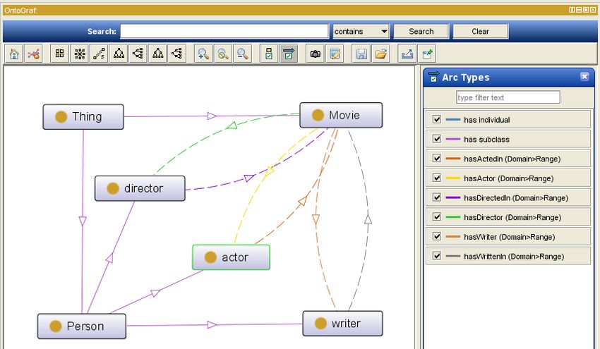
Appl. Sci. 2021, 11, 7104 4 of 25
on the neural network [11]. At present, recommendation algorithms have evolved from
classic collaborative filtering algorithms to methods that combine deep neural networks,
such as DeepFM, Deep&Wide and Alibaba’s XDeepFM model, which is currently used in
the majority of e-commerce websites. The recommendation algorithm based on a neural
network can automatically perform feature interaction. Furthermore, various features can
be continuously and autonomously learned and trained in the neural network to achieve
better results [12].
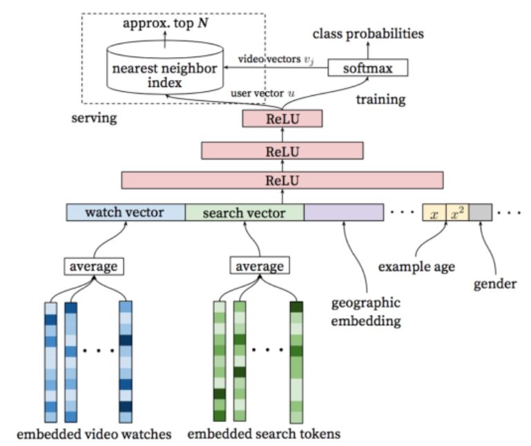
In the field of movie recommendation, YouTube’s recommendation technology has
been far ahead. Figure 1 is the framework diagram of the movie recommendation model
used by YouTube. It uses Word2Vec, ReLU, softmax, etc., to generate candidate sets. In
the recall phase, the value of the linear regression function is used as the sorting criterion
to recommend the highest ranked video for users. Furthermore, it can finally achieve
good results. This model is also a classic recall model in the history of recommendation
algorithm development.
Nowadays, more and more companies apply recommended technology to Internet
products. For example, the homepage of the current popular short video platform is a
feed stream composed of recommended models, which effectively increases the length of
stay and frequency of users. The application of the recommendation system has brought
great convenience to people. However, these recommended technologies also have many
problems such as data sparseness and cold start.
Figure 1. Frame diagram of YouTube recommendation model.
Recommendation system based on knowledge graphs: knowledge graphs have natu-
ral advantages in expanding entity information and strengthening the relations between
entities. It can provide a powerful and rich reference for recommendation systems. At the
beginning, the researchers directly applied the entity attributes in the knowledge graphs
to the recommendation algorithm. Then they produced feature-based knowledge graphs
assisted recommendation, that is, the introduction of knowledge graphs representation
learning. This method can provide deeper and longer-range associations between entities.
Subsequently, a structure-based knowledge graph recommendation model was produced.
The structure-based recommendation model can use the structure of the knowledge graphs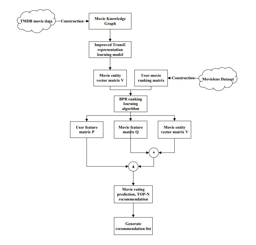
Appl. Sci. 2021, 11, 7104                                                                                            5 of 25

                            more directly. For example, it can perform a breadth-first search on each entity to obtain
                            multi-hop related entities nearby, and get recommendation results from it [13].
                                  In 2016, Hao Wang and other researchers proposed the CKE (Collaborative Knowledge
                            Base Embedding for Recommendation Systems) recommendation model, which aroused
                            widespread concern around the world. The model uses the TransR [14] representation
                            learning algorithm to obtain the structured information in the knowledge graphs. It uses
                            the encoder to obtain the visual and text representation vectors of the items, and introduces
                            them into the latent factor vectors of the items. Finally, it combines collaborative filtering
                            for recommendation [15]. In recent years, deep learning has been extremely popular,
                            and deep neural network recommendation algorithms based on knowledge graphs have
                            also been widely studied. In 2018, DKN (Deep Knowledge-Aware Network for News
                            Recommendation) proposed by Hongwei Wang and others for news recommendation [16]
                            is the representative algorithm.
                                  Knowledge graph recommendation system is applied to many fields, such as smart
                            social tv [17], personalized user recommendations [18–20], etc. However, in recent years,
                            the movie knowledge graph has only just started. Although many scholars have stud-
                            ied knowledge graphs for movie recommendations [21,22] and used graph databases
                            for recommendations [23,24], these studies still have many drawbacks and need to be
                            continuously studied. Due to the real-time, richness and particularity of movie data, the
                            movie knowledge graphs need to be continuously modified and improved to adapt to the
                            changing and complex data in different scenes. This has become the difficulty of movie
                            recommendation based on the knowledge graphs.

                            3. Construction of Movie Knowledge Graph
                            3.1. Knowledge Base Construction
                                  This article uses crawler to obtain movie data. We crawled the data in the “The Movie
                            Database (TMDb)” website. We correlated the movies to be crawled with the movies in
                            the MovieLens-1M dataset [25]. Finally, we crawled the relevant data of all the movies
                            involved in the MovieLens-1M dataset, and then sorted the data into CSV files.
                                  In order to construct the knowledge graphs, it is necessary to determine the elements
                            of the knowledge graphs. Through the analysis of relevant research, we have determined
                            several elements of the knowledge graphs in the field of movie, namely movies, actors,
                            directors, screenwriters and their basic information. We use them as the ontology of the
                            knowledge graphs.
                                  We use OWL language [26] for ontology representation. We mainly define four entities,
                            namely movie entity, screenwriter entity, director entity and actor entity, which are divided
                            into two entity concepts: movie and contributor. Entity attributes in ontology are mainly
                            divided into two categories, namely object attributes and data attributes, such as the object
                            attributes of a movie entity include hasActor relation, Actor etc., and data attributes include
                            MovieGenre, MovieYear, etc. Then, we define several relations between entities: movie-
                            director relation, movie-screenwriter relation, movie-actor relation and its inverse relation.
                            Finally, we use OWL language to describe the ontology library we have built.
                                  We use OWL 3.4.2 and Protege 5.0 to build our ontology library. After we use the
                            Protege tool to build the ontology library, we can visualize its structure diagram in the
                            OntoGraf toolbar, as shown in Figure 2.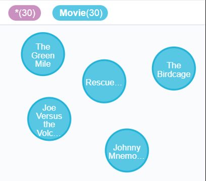
Appl. Sci. 2021, 11, 7104                                                                                         6 of 25

                            Figure 2. Structure diagram of the ontology library.

                                  In the ontology library structure diagram, in order to express the structure of the
                            knowledge graphs more clearly, we have derived three entity classes, namely actor, writer,
                            and director entity under the Person entity class, so that the relation between the three
                            and the Movie entity class and the inverse relation can be shown more vividly. At the
                            same time, in order to make the structure diagram more concise, we did not show the data
                            attributes of the entities in it.

                            3.2. Building a Knowledge Graph Based on Neo4j
                                 We choose Neo4j [27,28], a non-relational database, to store and display data. Figure 3
                            shows a partial screenshot of the visualized knowledge graph. The blue ones are movie
                            entities and the purple ones are contributor entities. The relations between entities are
                            marked with arrows and the information on it.

                            Figure 3. Partial display of knowledge graphs.

                            (1)   Figure 4 shows several random movie entities in the knowledge graph. The picture
                                  only shows five movie entities.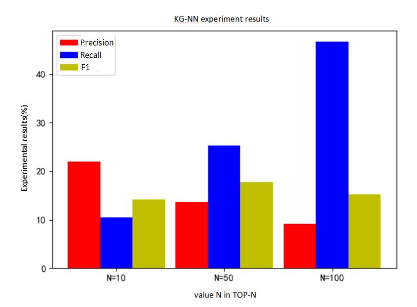
Appl. Sci. 2021, 11, 7104                                                                                        7 of 25

                            Figure 4. Example of movie entity.

                            (2)   Figure 5 shows the set of all entities connected to a random movie entity in the
                                  knowledge graph. The picture shows the relations between the entities of the movie
                                  “Top Gun” and various contributors, including actors, directors and screenwriters.

                            Figure 5. Example of movie-contributor entity relation.

                            (3)   Figure 6 shows the use of Cypher [29,30] to query the shortest path between two
                                  entities. The picture shows the shortest path between the two actors Cuba Gooding Jr.
                                  and Keanu Reeves.
Appl. Sci. 2021, 11, 7104 8 of 25
Figure 6. Shortest path query.
4. Movie Recommendation Model Based on Knowledge Graph
Representation Learning
In this section, we use the improved TransE [5] model to vectorize the knowledge
graphs constructed above [31]. We obtain the low-dimensional dense vectors corresponding
to entities and relations. After that, two recommendation methods based on knowledge
graphs are proposed, which combine knowledge graphs with Bayesian personalized
ranking learning and deep neural networks.
4.1. TransE Algorithm Improvement
4.1.1. TransE Algorithm Introduction
The algorithm can effectively vectorize the knowledge in the graph. We define h as
head, r as relation, and t as tail. The specific idea of the TransE algorithm is shown in
Figure 7. It hopes that the two entity vectors can be connected by a relation vector, that is,
h + r ≈ t.
Figure 7. TransE algorithm description diagram.
The scoring function of the TransE algorithm is shown in Formula (1). This function
uses Euclidean distance to quantitatively describe the embedding error of entities and
relations, where k ∗ k2 represents the 2 norm of the vector, that is, the Euclidean distance.
f r (h, t) =k h + r − t k2 2 (1)
The TransE algorithm uses the idea of maximum interval to train the margin-based
ranking loss as the objective function, as shown in Formula (2). Among them, S is all
the triples in the knowledge graphs. S’ is the negative example triples we constructed. γ
represents the margin, which is used to control the distance between positive and negative
samples. It is generally set to 1.
L= ∑ ∑ max(0, fr (h, t) + γ − fr (h0 , t0 )) (2)
(h,r,t)∈S(h0 ,r 0 ,t0 )∈S0 (h,r,t)Appl. Sci. 2021, 11, 7104 9 of 25
The TransE algorithm randomly initializes the entity vector and the relation vector
before model training. It performs normalization processing. The algorithm uses the
stochastic gradient descent algorithm based on the loss function shown in Equation (2)
to solve the minimum value of the objective function. Finally, the model will generate
a d-dimensional vector for the entities and relations in the triple according to the vector
dimension d we input.
4.1.2. Improvement of Negative Triples Construction Method
In the training process of TransE algorithm, correct triples and wrong triples are
needed. These wrong triples are also called negative triples. We need to construct them
ourselves. We propose corresponding improvements to the deficiencies of the original
negative sampling algorithm in the TransE model.
The original negative triple construction process of the TransE algorithm is as follows:
Firstly, randomly select a triple existing in the knowledge graphs, that is, the correct triple
(h, r, t). Then randomly select one or two entities from the knowledge graphs. In our
experiment, we randomly select a movie entity or a contributor entity, and use them
as the head entity h’ or the tail entity t’ to form a negative triple (h’, r, t’). However,
this construction method has an obvious shortcoming. That is, it is very likely that the
constructed negative triples are still correct triples. This situation is more common in
many-to-one, one-to-many, and many-to-many relational mapping types. For example,
the correct triple (Marvel’s The Avengers I, hasActor, Robert Downey, Jr.) may generate
negative triple (Marvel’s The Avengers II, hasActor, Robert Downey, Jr.) after sampling
in this way. However, the negative triple is correct, which affects the training effect of
the model.
In order to solve the above problem, we use the Bernoulli sampling algorithm to
randomly select entities. The improved negative triple construction process is as follows:
First, for each triple connected by the relationship r, we count the average number of
tail entities corresponding to the head entities and the average number of head entities
corresponding to the tail entities, denoted as M1 and M2, respectively. Then, we calculate
the probability P according to Formula (3) and use it as a parameter of the Bernoulli
distribution to extract entities. In this way, different methods of extracting entities will be
obtained in different relational mapping types.
M1
P= (3)
M1 + M2
The extraction method obtained according to the above method is shown in Table 1.
Table 1. Sampling methods for different relation mapping types.
Relation Type Condition Extraction Method
The negative triple generated by replacing the tail entity is more
likely to be a positive example, so the head entity is replaced with a
One to many M1 ≥ 1.5 and M2 < 1.5
greater probability P. The tail entity is replaced with a smaller
probability 1 − P.
The negative triple generated by replacing the head entity is more
likely to be a positive example, so replace the tail entity with a
Many to one M1 < 1.5 and M2 ≥ 1.5
greater probability P. The head entity is replaced with a smaller
probability 1 − P.
Consider the number of head entities and tail entities. Replace
Many to many M1 ≥ 1.5 and M2 ≥ 1.5
position entities with a small number.
4.1.3. Training Process Improvement
We introduce the idea of network feature structure learning into the TransE algorithm.
We use the method of hybrid feature learning. Furthermore, we use the feature struc-Appl. Sci. 2021, 11, 7104 10 of 25
ture information of entities in the knowledge graphs to improve the overall effect of the
TransE model.
First, we build a three-layer neural network. The input of the neural network is the
neighbor entity set and relation set of a specific entity. Through the middle projection layer,
we sum the input information and output our target entity. The specific model structure of
the neural network is shown in Figure 8.
Figure 8. Neural network model structure diagram.
Among them, the input (h1, r1) (h2, r2) (h3, r3). . . are all entities and relations con-
nected to a specific entity. The summation formula of the projection layer is shown in
Formula (4). The intermediate vector Xt generated by the projection layer is used as the
representation vector of the adjacency structure we have learned.
Xt = ∑ V ( h ) + V (r ) (4)
(h,r )∈ N (t)
The feature learning of the neighbor structure takes the prediction probability as the
learning objective. The loss function is shown in Formula (5), where E represents the set of
entities in the knowledge graphs, and N (t) represents the adjacent structure information
of the specific entity node t, that is, the input data of the neural network.
Lt = ∑ log p(t | N (t)) (5)
t∈ E
We use softmax to calculate the probability in the loss function. The calculation for-
mula is shown in Formula (6). Among them, y(t) represents the un-normalized probability
value of the entity t, as shown in Formula (7). b and U are the parameters of softmax, which
are constantly changing during the training of the model.
ey(t)
p(t | N (t)) = (6)
∑e∈ E ey(e)
y(t) = b + UXt (7)
We mainly study the first-order neighbor information of each entity, that is, context
information with a step length of 1.
Then, on the basis of the TransE algorithm, we use the adjacent structure information
of each entity as a supplement. We use a hybrid feature learning method to improve our
model. The improved loss function is shown in Formula (8).Appl. Sci. 2021, 11, 7104 11 of 25
L = L1 + L TransE (8)
Among them, L1 is the loss function of the above-mentioned neighbor structure feature
learning. L TransE is the loss function of the TransE model, as shown in Formula (9).
L= ∑ log p(t | N (t)) + ∑ ∑ max(0, fr (h, t) + γ − fr (h0 , t0 )) (9)
(h,r,t)∈S (h,r,t)∈S(h0 ,r 0 ,t0 )∈S0 (h,r,t)
Through the loss function, we can see that the improved algorithm has two parts. The
first part uses the nearest neighbor vector to predict the target entity so that representation
learning can make full use of the structural information in the knowledge graphs. The
second part is the training process of the TransE algorithm. In order to allow them to share
the representation vector, we adopt a cross-training mechanism of information sharing.
In the iterative process of model optimization, we use the Hierarchical Softmax al-
gorithm [31,32]. First, a Huffman tree is constructed. The entities and relations are the
leaf nodes of the tree. The frequency of their appearance in the triple set is used as the
weight of the node. Therefore, the high-frequency entities and relations are near the root
node of the tree. We treat each branch in the path from the root node to the leaf node as a
binary classification and generate a probability value. These probabilities are multiplied to
obtain the p(t | N (t)). We use this method to calculate the p-value. The specific calculation
formula is as follows:
lt
p(t | N (t)) = ∏ p ( d j t | Xt , θ j t ) (10)
j =1
Among them, l t is the number of branches in the path from the root node to the entity
or relation t. Xt and θ j t are the intermediate vector and auxiliary vector, respectively, which
are obtained during the training process of the model. The calculation of p(d j t | Xt , θ j t ) is
shown in Formula (11).
( )
t t σ ( Xt θ j t ), d j t = 1
p ( d j | Xt , θ j ) = (11)
1 − σ ( Xt θ j t ), d j t = 0
Among them, d j t = 1 means that the j-th branch in the path from the root node to the
leaf node t is a positive class. Otherwise, d j t = 0 is a negative class. σ is a sigmoid function.
After calculation, a probability value of 0 to 1 is output.
4.1.4. Improved Algorithm
The improved TransE model still uses the stochastic gradient descent algorithm to
solve the loss function. It continuously update the parameters and vector information
through the back propagation algorithm. The specific steps are shown in Algorithm 1.
V (h) = V (h) + α ∗ ∂L TransE /∂V (h)
V (r ) = V (r ) + α ∗ ∂L TransE /∂V (r ) (12)
V (t) = V (t) + α ∗ ∂L TransE /∂V (t)
The algorithm continuously updates the shared vector V of entities and relations
through Formula (12). This part is the original part of the TransE algorithm. The values of
some parameters in the equation will be discussed in Section 5.
θj t = θ j t + α ∗ ∂L1 /∂θ j t
(13)
u = u + α ∗ ∂L1 /∂Xt
We continuously update the vector information of the nearest neighbor structure
feature of the entity t through Formula (13). The 14th line of the algorithm indicates that
the gradient u is contributed to the shared vector corresponding to all entities and relations
in the nearest neighbor structure of the entity t.Appl. Sci. 2021, 11, 7104 12 of 25
Algorithm 1: Improved TransE algorithm.
Input: movie triple training set S, vector dimension d, margin γ and learning rate α
Output: entity vector and relation vector with dimension d
1: Construct a Huffman tree based on the set of triples S.
2: Initialize the shared vector V of entities and relations.
3: for total number of training rounds do
4: for each correct triple (h, r, t) in the triple training set S do
5: for negative triples constructed using Bernoulli distribution (h0 , r, t0 ) do
6: Update V (h), V (r ), V (t) using back propagation and gradient descent
algorithm according to Formula (12).
7: end for
8: Get the nearest neighbor structure information N (t) of the entity t, and use
the accumulation method to get Xt .
9: Initialization vector u = 0 .
10: for Number of branches l t do
11: According to Formula (13), use back propagation and gradient descent
algorithm to update θt j and u.
12: end for
13: for N (t) do
14: V (e) = V (e) + u, where e represents the entity and relation node in N (t).
15: end for
16: end for
17: end for
4.2. KG-BPR Recommend Model
This paper proposes a movie recommendation algorithm that combines knowledge
graphs and Bayesian Personalized Ranking (BPR), referred to as KG-BPR. BPR is a person-
alized recommendation model based on ranking learning [33–35]. It is an improvement of
the matrix factorization algorithm. It mainly models the relative preference ranking of two
different items, and obtains the user feature matrix and item feature matrix through the
user-item ranking data.
The flow chart of the KG-BPR model is shown in Figure 9. First, we use the improved
TransE representation learning method to obtain the entity vector and relation vector
corresponding to the knowledge graphs. Then, we integrate the movie entity vector matrix
into the BPR model, that is, by introducing the external hidden information of the movie to
assist the generation of feature matrix based on user-behavior data. Finally, we can get the
model parameters based on the maximum posterior estimation, that is, the user feature
matrix and the movie feature matrix. After the model training is completed, the user’s
preference value for the movie is obtained through the two generated matrices and the
movie entity vector matrix. The movie recommendation list is generated according to the
value, and each user can get the recommended movies.
We use V to represent the embedding vector matrix obtained by the representation
learning model. The size of V is n ∗ k, where n is the number of movies and k is the
dimension of the embedding vector. First, we construct a set of (u, i, j) triples, which means
that for user u, their interest in movie i is greater than their interest in movie j. These sets
of triples are the data sets required for KG-BPR model training, and are denoted by D in
the following. In addition, we need to make two assumptions about these data. First, each
user’s preference behavior is independent of each other, that is, whether user u likes movie
i or movie j has nothing to do with other users. Second, the partial order of the same user
for different movies is independent of each other, that is, whether user u likes movie i or
movie j has nothing to do with other movies.Appl. Sci. 2021, 11, 7104 13 of 25
Figure 9. KG-BPR model recommendation flowchart.
After that, the KG-BPR model uses the idea of matrix decomposition to decompose
the user-movie prediction ranking matrix X generated by the above steps. Furthermore,
it combines the movie entity vector V to obtain the user feature matrix P and the movie
feature matrix Q. Among them, the embedding dimensions of these matrices are consistent.
We assume that there are m users and n movies in the data set, and the dimension of the
feature matrix is k. Then, the size of the user feature matrix is m ∗ k. The size of the movie
feature matrix is n ∗ k, as is shown in Formula (14).
X = Pm∗k ( Qn∗k + Vn∗k ) T (14)
At the same time, the preference of user u for movie i is calculated as shown in
Formula (15).
k
xui = pu • (qi + vi ) = ∑ p u f ( qi f + vi f ) (15)
f =1
Among them, pu represents the u-th row of the user feature matrix P, that is, the
potential feature vector of user u. qi represents the i-th row of the movie feature matrix Q,
that is, the potential feature vector of movie i. vi represents the entity vector of movie i
generated by the improved TransE model.
The KG-BPR model uses the maximum posterior estimation to solve the model pa-
rameters, namely the matrix P and the matrix Q. For convenience, we use θ to represent
parameters P and Q. According to Bayesian formula, the model optimization goal is shown
in Formula (16).Appl. Sci. 2021, 11, 7104 14 of 25
P (i >u j | θ ) P ( θ )
∏ P(θ | i >u j) = ∏ P (i >u j )
(16)
(u,i,j)∈ D (u,i,j)∈ D
Among them, i >u j represents the preference relation of user u for movie i and movie
j, that is, the interest of user u in movie i is greater than the value of interest in movie
j. In the above, we assume that the user’s preference ranking for movies has nothing to
do with other users and movies. Then the above optimization goal is transformed into
Formula (17).
∏ P ( θ | i >u j ) ∝ ∏ P (i >u j | θ ) P ( θ ) (17)
(u,i,j)∈ D (u,i,j)∈ D
It can be seen from Formula (17) that the optimization goal of the KG-BPR model
is divided into two parts. The first part is related to the sample data set, and the latter
part is irrelevant. For the first part of the optimization goal, the calculation formula of the
probability value P(i >u j | θ ) is shown in Formula (18).
1
P(i >u j | θ ) = σ ( xuij (θ )) = − xuij (θ )
(18)
1+e
Among them, σ( x ) is the sigmoid function. xuij represents the preference difference of
user u for movie i and movie j. The greater the difference, the better the model effect. We
use the simplest difference calculation to reflect this difference, as shown in Formula (19).
xuij (θ ) = xui (θ ) − xuj (θ ) (19)
In summary, the first part of the calculation process of the KG-BPR model optimization
objective is shown in Formula (20). At the same time, we can see that the idea of the first
item in the optimization goal is very simple. For (u, i, j) in the training data set D, if the
user prefers movie i, then in the user-movie ranking matrix, the value xui is greater than
xuj . The greater the difference, the better.
∏ P (i >u j ) = ∏ σ ( xui − xuj )
(u,i,j)∈ D (u,i,j)∈ D
= ∏ σ ( p u • ( qi + vi )
(u,i,j)∈ D
− pu • (q j + v j ))
(20)
k
= ∏ σ ( ∑ p u f ( qi f + vi f )
(u,i,j)∈ D f =1
k
− ∑ pu f (qi f + vi f ))
f =1
We assume that the prior distribution of the model parameter θ is shown in Formula (21).
Assuming it is a normal distribution, the second part of the optimization objective of the
KG-BPR model is equivalent to adding a regular term, as shown in Formula (22).
P(θ ) ∼ N (0, λθ I ) (21)
ln P(θ ) = λ k θ k2 (22)Appl. Sci. 2021, 11, 7104 15 of 25
Therefore, the final optimization goal of the KG-BPR model, that is, the maximum
logarithmic posterior estimation function is shown in Formula (23).
ln P(θ |i >u j) ∝ ln P(i >u j|θ ) P(θ )
= ln ∏ σ ( xui − xuj ) + ln P(θ )
(u,i,j)∈ D
= ∑ ln σ ( xui − xuj ) + λ k θ k2
(u,i,j)∈ D
(23)
k
= ∑ ln σ ( ∑ pu f (qi f + vi f )
(u,i,j)∈ D f =1
k
− ∑ pu f (q j f + v j f )) + λ k θ k2
f =1
Finally, we take a negative value for the above formula. Using the gradient descent
method, we solve the model parameters by obtaining the partial derivative of the two
matrices. At last, we obtain the final user feature matrix P and the movie feature matrix Q.
4.3. KG-NN Recommend Model
This section proposes a movie recommendation algorithm that combines knowledge
graphs and neural network, referred to as KG-NN.
The main steps of the KG-NN algorithm are as follows: we first use the improved
TransE representation learning method in Section 4 to obtain the entity vector and the
relation vector. After the embedding layer, the user data and movie data are, respectively,
generated corresponding embedding vectors. Then input the movie entity vector generated
by the learning process as auxiliary information into the neural network together. After
that, it is the MLP fully connected layer, ReLU activation function and so on. In order to
predict the user’s interest in the movie, we combined the user-movie real rating data and
Adam optimization method for iterative training. Finally, the rating values of the model
training are used to sort from large to small to generate a movie recommendation list.
The flow chart of the KG-NN model in the movie recommendation process of this
article is shown in Figure 10. The input of the KG-NN model mainly has two types. The
first type is the embedding vector generated by the basic user data and movie data through
the embedding layer. The second type is the movie entity vector generated by the improved
TransE representation learning algorithm.
According to the above introduction, we have generated the embedding vector corre-
sponding to the user data and the movie data. We stitch the movie data embedding vector
and the movie entity vector horizontally, then stitch it horizontally with the user data
embedding vector and input it into the fully connected layer. Through the fully connected
neural network for dimensional transformation and feature extraction, we can learn the
hidden vectors of users and movies and retain useful information in the neural network. A
ReLU function is immediately followed by each fully connected layer.
Finally, the output value obtained by the last fully connected layer of the model is
returned to between zero and one after the sigmoid function, as shown in the following
formula. Since users in the movie data set rated movies on a five-point scale, we also
normalized it to a value between zero and one to get yt .
1
y p (i) = sigmoid( xi ) = (24)
1 + e − xi
Among them, xi represents the weighted output of the last fully connected layer. Then
compare it with the normalized user-movie rating data yt , and use cross entropy as the loss
function. The entire model is trained iteratively with Adam optimizer. The loss function is
shown in Formula (25).Appl. Sci. 2021, 11, 7104 16 of 25
n
1
Loss = −
n ∑ (yt (i) log y p (i) + (1 − yt (i) ) log(1 − y p (i) )) (25)
i =1
Among them, y p is the predicted score of the KG-NN model. yt is the normalized real
score, and n is the total number of user-movie score data in the training set.
In order to prepare for the final movie recommendation, the model needs to predict
the rating value of the movie for each user, and decide whether to recommend the movie
to the user according to the calculated score.
We finally get the parameters of the entire KG-NN model. When performing TOP-N
recommendation, we use the entire model to predict the user’s ratings of unseen movies.
We sort the predicted ratings in descending order, and extract the top N after sorting [36].
Movies are recommended to users as a recommendation list.
Figure 10. KG-NN model process framework diagram.
5. Experiment
5.1. TransE Model before and after Improvement
5.1.1. Experiment Setup
The data required for the experiment comes from the data in the knowledge graphs
we constructed previously. For ease of use, we use APOC technology to export the dataAppl. Sci. 2021, 11, 7104 17 of 25
in the Neo4j graph database into a csv type relational file. Furthermore, a unique id is
generated for all entities and relations. Finally, the entity-to-entity-id mapping file, the
relation-id mapping file and the triple file are generated. We split the triple file into a
training set, a validation set and a test set at a ratio of 8:1:1.
In the knowledge graph representation learning algorithm, we use the average ranking
MeanRank and the top ten percentage hits@10 to evaluate the quality of the model.
For each test triple (h, r, t), we replace h or t with each entity in the knowledge graphs.
Then, we calculate the score value by the formula 1 score function. We arrange the scores
in ascending order. The smaller the score, the closer the entity is to the tail entity of the
original triple. Among them, MeanRank refers to the average ranking of the correct triples,
that is, the average number of serial numbers of the correct tail entities in the above score
sequence after all the test triples are calculated by the above steps.
Then we observe whether the position corresponding to the correct entity in the test
triple is in the top ten of the above score sequence. If it is, the count is increased by one.
The number of triples in the top ten/total number of triples is hits@10, which represents
the probability that the correct triple is in the top 10.
5.1.2. Analysis of Results
We compare the TransE algorithm with our improved TransE algorithm for analysis.
In the experiment, we set the generated vector dimension of the two models to 100. The
learning rate is set to 0.01. The remaining parameters mentioned in this paper are set to the
default values. We first observed the changes in the loss functions of the two models and
found that the loss function of the TransE model became stable after about 130 iterations,
while the improved TransE model became stable after about 160 iterations. At the same
time, the loss function value of the improved TransE model is significantly smaller than the
that of the TransE model. However, the loss functions of the two models are different, so
we cannot judge the pros and cons of the model only from the value of the loss function.
In addition, we studied the influence of the embedding dimensions of entities and
relations in the TransE algorithm on the experimental results. We selected the embedding
dimensions with values of 20, 50, 80, 120, 150, and 200. The obtained MeanRank value and
hits@10 value are shown in Figures 11 and 12.
Figure 11. MeanRank values under different embedding dimensions.Appl. Sci. 2021, 11, 7104 18 of 25
Figure 12. Hits@10 values under different embedding dimensions.
Under normal circumstances, the better the model effect, the smaller the MeanRank
value and the larger the corresponding hits@10 value. It can be seen from Figure 11 that
when the embedding dimension is low, the MeanRank value is relatively large, that is, the
correct triples are lower in the sorting. As the dimension increases, the MeanRank value
keeps decreasing, and reaches the minimum when the dimension is 120. The minimum
value is about 229. After that, it keeps getting bigger.
It can be seen from Figure 12 that when the embedding dimension is low, the value
of hits@10 is smaller. As the dimension increases, the value of hits@10 becomes larger.
When the dimension is 120, it reaches the maximum value of about 0.82. After that, it keeps
getting smaller.
At the same time, we also did experiments similar to the above process on the im-
proved TransE model. After multiple experiments under different parameter combinations,
we determined the optimal parameter combination according to the MeanRank value and
hits@10 value. In the model training process, the number of iterations in is 200. The best
combination we get is that the embedding dimension of entities and relations is 100, the
learning rate is 0.01, and the margin γ is 1. We calculated the MeanRank value and hits@10
value of the improved TransE model based on the above parameter combination. The
experimental results are shown in Table 2 and Figure 13.
Figure 13. Comparison of MeanRank value and hit@10 value before and after improvement.Appl. Sci. 2021, 11, 7104 19 of 25
Table 2. Comparison of MeanRank value and hit@10 value before and after improvement.
Model MeanRank Value hits@10 Value
TransE model 229.21078 0.81862
Improved TransE model 189.50092 0.86336
It can be seen from the above table that the MeanRank value and hits@10 value of the
improved TransE model are about 189 and 0.86, respectively. Compared with the transE
model, both of them have been significantly improved. The MeanRank value is reduced by
about 30. The value of hits@10 increased by approximately 0.04.
It can be seen that the TransE algorithm performs better in the one-to-one relational
mapping type, but does not perform well in the many-to-one and many-to-many relational
mapping types. Therefore, this will be analyzed specifically in the future.
5.2. KG-BPR Model and KG-NN Model
5.2.1. Experiment Setup
This paper uses MovieLens-1M as the experimental data set.
The detailed information is shown in Table 3:
(1) user.dat: This file contains the basic information of the user, such as user ID, gender,
age, occupation, etc.
(2) movie.dat: This file contains the basic information of the movie, such as movie ID,
name, type, etc.
(3) rating.dat: This file contains the user’s rating information for the movie.
Table 3. Information of MovieLens-1M dataset.
Number of Users Number of Movies Number of Ratings Data Density
6040 3382 756,684 3.704%
We split the data set into training set and test set at a ratio of 7:3. In the KG-BPR model,
it is necessary to construct a set of partial order relations (u, i, j) before establishing the
user-movie prediction ranking matrix. In order to ensure the accuracy of the data, that is,
the interest of user u in movie i is indeed greater than that in movie j, we let i be a movie
with a user rating of 5 and j is a movie with a user rating below 5 or no rating. At the
same time, in the experiment, we used precision, recall, F1 value and MAP to evaluate the
performance of the recommendation.
5.2.2. KG-BPR Experiment Results and Analysis
We first observe the influence of the feature dimension d on KG-BPR model. We set
dimension d to 20, 40, 60, 80, 100, and 120. We set N of the TOP-N recommendation model
to 100, which means 100 movies are recommended for each user. We set the learning rate
of the improved TransE model to 0.01. The regularization coefficient of the entities and
relations vector is set to 0.1. The learning rate of the KG-BPR model is set to 0.01. The
regularization coefficient of the user feature matrix and the movie feature matrix is set to
0.01. Furthermore, the maximum number of iterations is 1000. The ratio of the training set
and test set is 7:3. The experimental results are shown in Table 4 and Figure 14.
It can be seen from Table 4 that when the dimension d is 40, the KG-BPR model has the
best effect and the MAP value is the largest, which is 0.04807176. Through comparison, it
can be found that due to the introduction of knowledge graphs in KG-BPR model, the MAP
value of the KG-BPR model is improved in any feature dimension and the recommendation
effect is better compared with BPR model.Appl. Sci. 2021, 11, 7104 20 of 25
Table 4. MAP values of models in different dimensions.
Feature Dimension d KG-BPR Model MAP Value BPR Model MAP Value
20 0.04735185 0.04632617
40 0.04807176 0.04506615
60 0.04802097 0.04605486
80 0.04767749 0.04557344
100 0.04781234 0.04514578
120 0.047412 0.04507794
Figure 14. The MAP value of the model in different dimensions.
During the experiment, we found that after introducing the movie entity vector
generated by the knowledge graphs, the number of iterations required for the model to
achieve the optimal effect is greatly reduced. Therefore, we set the dimension d to 40
and observe the effect of the KG-BPR model as the number of iterations increases. The
experimental results are shown in Figure 15.
Figure 15. Effect diagram of MAP value changing with iteration times.Appl. Sci. 2021, 11, 7104 21 of 25
It can be seen from Figure 15 that the MAP value of the KG-BPR model has stabilized
after about 40 iterations, while the BPR model needs to be iterated about 150 times before it
stabilizes. Therefore, the introduction of the movie entity vectors speeds up the training of
model parameters. Furthermore, it can assist the model to generate user feature matrices
and movie feature matrices for recommendation faster and better.
Finally, we compared the KG-BPR model with other models. The comparison results
of the MAP value of the model are shown in Table 5. Among them, NMF and SVD are
implemented using the Python-based open source library SupriseLib. The MAP value in 5
is when the N value is 100 in the Top-N recommendation.
Table 5. Comparison experiment results.
Model MAP Value(%)
KG-BPR 4.81
BPR 4.5
NMF 4.39
SVD 2.95
It can be seen that using the semantic information of the item itself efficiently and
introducing the auxiliary information of the knowledge graphs, KG-BPR model effectively
improves the performance of the recommendation. It produces a high-quality recommen-
dation list, and greatly improves the ranking effect in the recommendation list.
5.2.3. KG-NN Experiment Results and Analysis
In the KG-NN model, the vector dimension of the input data after the embedding layer
is set to 100. The entity vector and relation vector dimensions generated by the improved
TransE model are also set to 100. The number of samples selected for each iteration, namely
batch_size, is set to 512. Finally, we use the Adam algorithm to continuously optimize the
loss function.
First, we studied the influence of the number of fully connected layers in the model.
The relevant parameters are set as shown above. We set the number of fully connected
layers to 3, 4, 5, 6, 7, 8, and 9. We recommend 10 movies for each user, that is, N in the
TOP-N recommendation model is set to 10. The precision, recall and F1 values obtained in
the experiment are shown in Table 6 and Figure 16.
Figure 16. The effect of the number of fully connected layers on the experimental results.Appl. Sci. 2021, 11, 7104 22 of 25
Table 6. Experimental results under different K values.
Number of Fully Connected Layers K Precision(%) Recall(%) F1(%)
3 19.0 9.078 12.286
4 19.1 9.207 12.425
5 19.6 9.474 12.774
6 20.4 10.167 13.571
7 21.3 10.204 13.798
8 20.8 10.094 13.592
9 19.7 9.497 12.816
It can be seen from Table 6 that the trend of precision, recall and F1 value is roughly
the same as the trend of the number of fully connected layers. When the number of fully
connected layers is 7, the effect is the best. At this time, the precision reaches 21.3%, the
recall rate reaches 10.204%, and the F1 value reaches 13.798%. When the number of fully
connected layers is 9, the model is over-fitted and the performance decreases.
Then, we set the number of fully connected layers K to 7. According to the other model
parameters mentioned above, we compared the effect of the model when N is different,
that is, the numbers of movies recommended for each user is different. We set N to 10, 50,
and 100, respectively. The experimental results are shown in Table 7 and Figure 17.
Table 7. Experimental results under different N values.
Value N in TOP-N Precision(%) Recall(%) F1(%)
10 21.3 10.204 13.798
50 13.674 25.318 17.757
100 9.08 46.635 15.2
Figure 17. Experimental results under different N values.
It can be seen from Table 7 that with the N value increases, the accuracy rate keeps
getting smaller, while the recall rate keeps getting larger. The F1 value has always been
within a reasonable range. Therefore, to some extent, when the N value is relatively large,
the model can still have a better recommendation effect.Appl. Sci. 2021, 11, 7104 23 of 25
Finally, we compared the KG-NN model with other models. The comparison result of
the model accuracy is shown in Table 8. The reason why the KG-NN model only compares
the precision with other models is that the recall rate of this model may be slightly lower
than that of the model to be compared. Generally, if a model has a high precision, the recall
rate may decrease slightly. It is best to find a balance between precision and recall, but
one of the most significant features of the KG-NN model is the improved precision, so the
precision is compared. Among them, the MLP model is a fully connected recommendation
model embedded, that is, the KG-NN model removes the part of the knowledge graph.
NMF, SVD and ItemKNN are implemented using the Python-based open source library
SupriseLib. The precision in Table 8 is the result when N of the Top-N recommendation
is 10.
Table 8. Comparison experiment results.
Model Precision(%)
KG-NN 21.3
MLP 11.6
NMF 11.5
SVD 4.69
ItemKNN 2.32
The experimental results show that the neural network recommendation model based
on the knowledge graphs has a good effect in TOP-N recommendation. Compared with the
neural network model that only relies on single data for recommendation, the recommenda-
tion model using knowledge graphs and deep neural network has a better recommendation.
6. Discussion and Conclusions
In this paper, we combine knowledge graphs with recommendation system. In tra-
ditional recommendation models such as collaborative filtering and matrix factorization,
various behavior data analysis and modeling of users are generally used to recommend
items. However, the introduction of knowledge graphs can provide a lot of additional
auxiliary information for personalized recommendation systems. It can also effectively
alleviating the cold start problem. Although the article only considers the construction
of knowledge graphs in the movie domain, the improved recommendation algorithm
proposed in this article is also applicable to many other areas, including product recom-
mendation, music recommendation, news recommendation, etc. The algorithm has strong
scalability and applicability.
Through the analysis and exploration of related movie data, we determined the
entities and relations of the knowledge graphs in the movie domain and completed the
construction of the ontology database. We obtained the required movie data through
crawler. We completed the construction of the knowledge graphs. Furthermore, we use
Neo4j graph database for storage and visual display.
We researched and analyzed the shortcomings of the classic TransE representation
learning algorithm, that is, it learns the triple data in isolation during the training process
but ignores the structural data and neighbor information in the knowledge graphs. There-
fore, we improved the TransE model to solve this problem. The improved model is trained
by cross iteration of triple data and knowledge graph structure data. It has effectively
improved the effect of learning.
At the same time, we combined the knowledge graphs with the ranking learning and
neural network, respectively, and proposed the KG-BPR model and the KG-NN model. We
conducted comparative experiments on them, respectively, verifying the feasibility of the
two models we proposed. At the same time, it shows that the auxiliary information of the
knowledge graphs has important value in the recommendation system.
However, because the knowledge graphs and recommendation system are particularly
complex, there are some shortcomings in our work. First of all, when constructing theYou can also read