Quantication of Mangrove Extent using a Combination of Optical and Radar Images in Google Earth Engine Platform: The case of Anlo Beach Wetland ...
←
→
Page content transcription
If your browser does not render page correctly, please read the page content below
Quantification of Mangrove Extent using a
Combination of Optical and Radar Images in Google
Earth Engine Platform: The case of Anlo Beach
Wetland Complex, Shama District, Western Region,
Ghana
Daniel Aja ( ajadaniel3611@gmail.com )
University of Cape Coast https://orcid.org/0000-0002-8849-381X
Michael Miyittah
University of Cape Coast
Donatus Bapentire Angnuureng
University of Cape Coast
Research
Keywords: Algorithm, Decision Trees, Cloud Cover, NDMI, Wetland, Ghana
Posted Date: April 8th, 2021
DOI: https://doi.org/10.21203/rs.3.rs-398182/v1
License: This work is licensed under a Creative Commons Attribution 4.0 International License.
Read Full License
Page 1/27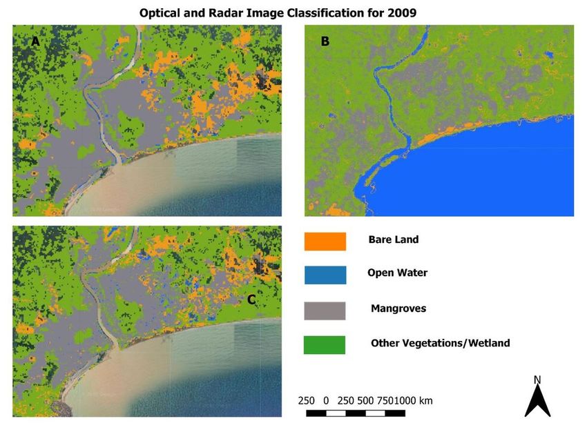
Abstract
Mangrove Forest classification in tropical coastal zones based on only passive remote sensing methods
is hampered by Mangrove complexities, topographic considerations and cloud cover effects among other
things. This paper reports on a novel approach that combines Optical Satellite images and Synthetic
Aperture Radar alongside their derived parameters to overcome the challenges of distinguishing
Mangrove stand in cloud prone regions. Google Earth Engine (GEE) cloud-based geospatial processing
platform was used to extract several scenes of Landsat Surface Reflectance Tier1 and synthetic aperture
radar (C-band and L-band). The imageries were enhanced by creating a function that masks out clouds
from the optical satellite image and by using speckle filter to remove noise from the radar data. The
random forest algorithm proved to be a robust and accurate machine learning approach for mangrove
classification and assessment. Our result show that about 16% of the mangrove extent was lost in the
last decade. The accuracy was assessed based on three classification scenarios: classification of optical
data only, classification of SAR data only, and combination of both optical and SAR data. The overall
accuracies were 99.1% (Kappa Coefficient =0.797), 84.6% (Kappa Coefficient = 0.687) and 98.9% (Kappa
Coefficient = 0.828) respectively. This case study demonstrates how mangrove mapping can help focus
conservation practices locally in climate change setting, coupled with sea level rise and related threats to
coastal ecosystems.

1. Background
Mangrove grows and flourishes in an environment that acts as a buffer zone for terrestrial and marine
ecosystems. They are globally important ecosystem that are restricted to coastal areas where mean
monthly air temperatures are higher than 20ºC and where there is no ice formation on the ground with
rare exceptions (Blasco et al., 2019). These ecosystems are made up of trees and shrubs that are found
in shallow sandy or muddy areas that are adapted to estuarine or saline environment (Erika et al., 2020).
They are truly unique because they are the only trees capable of tolerating large amount of salt and
water. This capability as well as surviving in low oxygen soil is a result of the root adaptations. Mangrove
forests occupy an insignificant proportion of land area (< 1%) but they are considered as the most carbon
abundant ecosystems within the tropics. Mangrove ecosystems have recently been included in the IPCC
climate mitigation strategy through a number of wetland supplements (Lucas et al., 2014).

In Africa, mangrove forests occupy roughly 2,746,500ha in 2010 (Bunting et al., 2018) and support
vulnerable coastal population by providing important ecosystem services such as natural sea defense,
mitigation of coastal erosion, water quality improvement as well as providing alternative livelihood
(Gedan et al., 2011; Kuenzer and Tuan, 2013; Lee et al., 2014; Mondal et al., 2018). Fatoyinbo and Simard
(2013) reported that mangrove cover about 7600ha along the coast of Ghana and seven major mangrove
varieties have been confirmed including Laguncularia racemose (white mangrove), Avicennia germinans
(black mangrove), Rhizophora harrisonii (Red mangrove), Rhizophora racemose (Red mangrove),
Rhizophora mangle (Red mangrove), Acrostichum aureum (golden leather fern) and Cornocarpus erectus
(botton mangrove) (Ellison et al., 2015; Nortey et al., 2016).
                                                  Page 2/27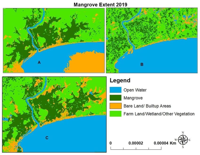
Despite providing many valuable services, these ecosystems have experienced significant degradation
and they are being threatened or lost (Alongi, 2012; Breithaupt et al., 2012). The rate of loss in the last two
decades have been estimated to double terrestrial rainforest loss over the same period (Mayaux, et al.,
2005). It is also estimated that about 2/3 of mangrove forest have been lost in the past century,
representing 1–8% mangrove loss per annum and at least 20–50 % global land area decline (more than
3.6 million ha) in the last 4–5 decades (FAO, 2007; Miththapala, 2008; World Mangrove Network, 2012).
The primary cause of mangrove loss has been deforestation for land conversion, primarily for
Aquaculture, Saltpans establishment and other Agricultural intensification.

Quantification of changes both in space and time for mangrove ecosystem is crucial for an improved
understanding of many coastal and sea processes. Conventional mapping of mangrove forest involves
huge capital for field work due to the difficulties associated with accessibility within the mangroves
ecosystem (Zhang et al., 2014). Space based technology such as remote sensing has a huge capacity to
map and monitor changes in mangrove forests owing to the fact that data can be captured from a
landscape which is otherwise difficult to access (Son et al., 2015). Several authors recommend the
combination of Synthetic Aperture Radar with Optical satellite data for more accurate quantification of
mangrove extent (Attarchi and Gloaguen, (2014); Ayman et al., 2017; Hu et al., 2020)

There have been several studies on mangrove extent across Africa (Kovacs et al., 2010; Salami et al.,
2010; Omo-Irabor et al., 2011; De Santiago et al., 2013; Fatoyinbo and Simard, 2013; Kuenzer et al., 2014;
Hoppe-Speer et al., 2015; Brown et al., 2016; Lagomasino et al., 2019), most of them largely concentrating
on few countries such as Gambia, Guinea-Bissau, Guinea, Mauritania, Mozambique, Madagascar, Nigeria,
Senegal, Sierra Leone, South Africa, and Tanzania. However, a good number of the studies are global in
nature but lack spatially explicit resolution suitable for locally tracking progress in the sustainable
development goals (SDGs) adopted by the United Nations (2030 agenda) and African Union (2063
agenda).

Mangroves support a range of SDGs, especially Goal 6 (Clean water and sanitation) and Goal 15 (‘Life on
Land’) (Fig. 2), as they serve as important indicators for monitoring progress locally, regionally and
globally. Specifically, indicator 6.6.1 (Change in extent of water-related ecosystems over time) of Goal 6
aims at protecting and restoring water-related ecosystems such as mangroves. While indicator 15.1.1 of
Goal 15 focuses on quantifying ‘forest area as a proportion of total land area’. Therefore, understanding
mangrove ecosystems and mapping their extent locally as well as globally is critical in meeting these
goals (Barenblitt and Fatoyinbo, 2020a). This can help coastal managers to focus conservation practices
and reduce the degradation of water-related ecosystems by improving our knowledge of these
ecosystems to drive action towards protection and recovery.

The coastline of Ghana, just like other coastal zones, faces imminent flooding, erosion and saltwater
intrusion as sea level rises. Mangroves in this area may be threatened by sea level rise. There is the need
to understand where mangroves are currently found and how they have changed over time by steady
monitoring and modelling of their vulnerability to either climate change or land use change. Therefore, the

                                                   Page 3/27
main objective of this case study is to map the temporal changes of Coastal-Wetland surface
characteristics and to show how mangrove mapping can help coastal managers to focus conservation
practices.

2. Materials And Methods
2.1 Study Location
This study was conducted at the Anlo Beach Wetland complex which is situated in the Shama District,
Western Region of Ghana as shown in Figure (1). The area covers about 50.42km2, lying approximately
within latitudes 5o 1' 30"N and 5o 3' 5"N, and longitudes 1°34'30"W and 1°37'30"W and it is covered by
mangroves which have been comparatively disturbed (Friends of the Nation. 2014). Hydrologically, the
area lies within the plains of Pra River, which opens directly into the ocean.

According to a study conducted in the location by Friends of the Nation (2014), the topography is largely
flat and the shoreline has an irregular sandy beach and the ocean areas are generally open and
characterized by pounding surf with medium to high energy. The coastline has eroded by an average of
100m in the last 50 years (Coastal Resources Center / Friends of the Nation, 2010). The wetland is largely
shallow (0.25–1.5 m) with fluctuating hydrology and chemical parameters.

The inhabitants of Anlo Beach community are predominantly fishermen with an estimated population of
about 2,231 consisting of 1,028 males and 1,203 females (Coastal Resources Center / Friends of the
Nation, 2010).

Figure 1: Map of Study Location

Figure 2: Key concepts related to sustainable development and links to the most relevant sustainable
development goals, targets, indicators and series

2.2 Datasets and Sources

                                                 Page 4/27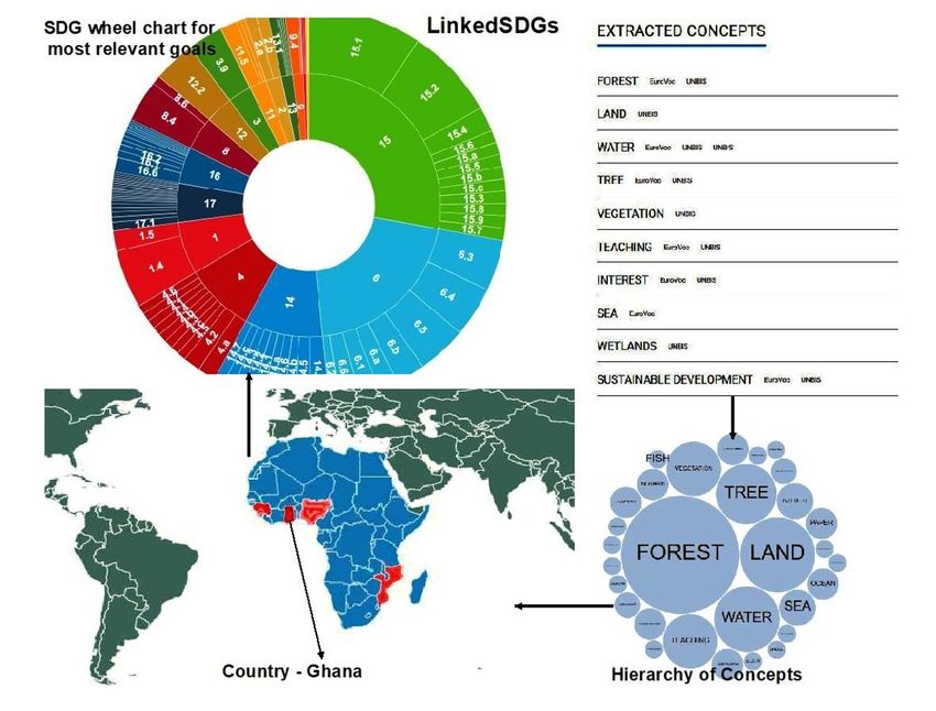
Table 1
                                Description of Datasets and their Sources
 S/N     Data Type      Description                                              Source

 1       Sentinel-1     C-band Synthetic Aperture Radar with Interferometric     Google Earth Engine
                        Wide Swath Mode (IW), Descending Pass, 25-meter          Platform Database
                        resolution, VV and VH polarization

 2       ALOS           L-band Synthetic Aperture Radar (SAR), 10x10             Japan Aerospace
         PALSAR-2       degrees in latitude and longitude, ortho-rectified,      Exploration Agency
                        slope corrected with pixel size approximately 25m by     (JAXA) EORC
                        25m. HH and HV polarization

 3       Landsat 8      Atmospherically corrected surface reflectance from       Google Earth Engine
         Surface        the Landsat 8 OLI/TIRS sensors, contain 5 visible        platform database
         Reflectance    and near-infrared (VNIR) bands, 2 short-wave
         Tier 1         infrared (SWIR) bands and 2 thermal infrared (TIR)
                        bands

 4       Landsat 7      Atmospherically corrected surface reflectance from       Google Earth Engine
         Surface        the Landsat 7 ETM + sensor containing 4 visible and      platform database
         Reflectance    near-infrared (VNIR) bands, 2 short-wave infrared
         Tier 1         (SWIR) bands and one thermal infrared (TIR) band
                        processed to ortho-rectified surface reflectance and
                        brightness temperature.

 5       SRTM DEM       Shuttle Radar Topography Mission which has               Google Earth Engine
                        undergone a void-filling process using the following     platform database
                        open-source data: ASTER GDEM2, GMTED2010, and
                        NED.

 6       Global         Global baseline map of mangroves distribution for        https://data.unep-
         Mangrove       2010                                                     wcmc.org/datasets/45
         distribution
         vector

2.3 Time Series of Mangrove Extent (Comparison of
Mangrove Extents)
2.3.1 Google Earth Engine
Data analyses for this study were performed using Google Earth Engine (GEE) cloud-based platform.
Google earth engine is a free open source cloud-based geospatial processing platform which comprises
of a catalogue of publicly available datasets e.g. Landsat imageries, Google computation power, an
application programming interface (API) as well as a code editor. GEE provides access to a variety of
satellite imageries from a number of NASA and ESA satellites including Landsat and Sentinel images. It
operates on a client versus server function where users can manipulate ‘proxy’ objects through the server
to send instruction to Google for processing and the results sent back to web browser for display. GEE
defaults to WGS84 projections with access to data at planetary scale.

2.3.2 Random Forest Classification
                                                Page 5/27
Random Forest Classification algorithm was applied in this study for mapping of mangrove extents. The
random forest classification is a type of machine learning that uses statistics to identify patterns in large
data sets. It is a type of artificial intelligence that learns from data and allows the user to process large
quantities of data to answer a particular research question. This is an ensemble tree based learning
algorithm that creates trees that are looking at a single pixel of a data with each tree looking at different
variables such as NDVI or different bands of Landsat images that help us to identify mangroves and
each tree is using that information to cast a vote. This decision trees select the best option based on how
many trees vote in one direction. It is a type of supervised machine learning classification.
2.3.3 Mangrove Extent Mapping
The images for the analysis were loaded into the Google Earth Engine code editor including Landsat8
surface reflectance tier1, Landsat7 surface reflectance tier1, SAR image (COPERNICUS), ALOS PALSAR
image, SRTM digital elevation and global mangrove distribution vector file. Note that the SRTM elevation
is from the shuttle radar topographic mission and it provides elevation and slope to narrow down the
study area to areas where mangroves are more likely to be found. The global mangrove distribution
vector was required to identify areas where Mangroves exist.

2.3.3.1 Optical Images (Landsat 7 & 8)
The map was setup by centering it to the area of interest, which in this case is the Anlo beach wetland
complex and its environs, using a geometry drawn over the area of interest. Then, the Landsat
composites were filtered to a cloud free mosaic (Fig. 3) by using a function that masks out clouds (Giri et
al., 2011; Hansen et al., 2013). Seven spectral indices: Normalized difference vegetation index (NDVI),
Normalized difference mangrove index (NDMI), Modified normalized difference water index (NDWI),
Simple ratio (SR), Ratio54, Ratio35, and Green chlorophyll vegetation index (GCVI) were added to the
Landsat imageries to provide information on not only vegetation in the pixels but also water content
because mangroves are found close to water (Shi et al., 2016; Nathan et al., 2018).

Figure 3: Cloud Free Landsat 8 Imagery

The Landsat data were filtered by date and region. This was done by setting up a temporal parameter by
creating a variable called ‘year’ and then indicating the required year. The mask function and the various
spectral indices were applied to the final image which has been narrowed down to the study area using
median reducer. Then the SRTM data was clipped to the study area (Landsat data) to further narrow
down to elevations less than 45m as mangroves occur mostly in low elevations. The NDVI and NDWI
masks were created by selecting the bands of interest (NDVI bands) to mask areas greater than 0.25, all
the indices range from − 1 to 1, areas that are greater than 0.25 are assigned to highly vegetative areas
and for NDWI, areas that are greater than − 0.5 were assigned.

Figure 4: False Color Composite of Landsat Image Clipped to Study Area

                                                   Page 6/27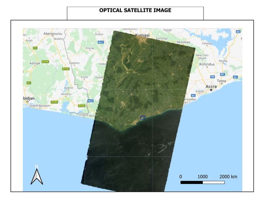
The visualization parameters were set and a false color composite (Fig. 4) was generated using B5, B6
and B4 combination. Then, the composite was added to the layer bar for visualization. This process was
performed for Landsat 8 (2019) imagery and Landsat 7 (2009) imagery.

2.3.3.2 Synthetic Aperture Radar (C-band & L-band)
Then, the Sentinel-1 database was loaded and filtered for images that are in interferometric wide swath
mode (IW), descending pass, 25m resolution and VV polarization. The code queries the Sentinel-1
database (COPERNICUS) and filter according to instrument mode and polarization. It is important to note
that the Sentinel-1 data set in Google earth engine is image analysis ready as it has been processed
already by implementing formal noise removal, radiometric and terrain correction. The values of PALSAR
data set are still in Log10 which must be converted to decibel (db) (Lavalle & Wright, 2009) using the
formula below.

γ0 = 10log10(DN2) + CF.............1

Where γ0 = Sigma naught (dB), DN = pixel value (digital number), CF (Calibration Factor) = -83.0 for the
PALSAR images.

The same process is repeated for VH polarization. The entire data set was filtered to get the desired date
(2019).

Figure 5: Filtered Synthetic Aperture Radar Image

The filtered images (Fig. 5) were added to the layer bar in order to display them for visualization. The
same procedure was followed to load ALOS PALSAR 2009 image which corresponds to the Landsat 7
image date. Now that both the SAR and Landsat imageries have been identified, the next thing was to
apply speckle filter to the SAR data to reduce noise.

2.3.4 Construction of Random Forest Model
Training samples were selected for four different land cover classes (Open water, Mangrove, Bare land
and other vegetation/Wetland) in order to perform a supervised classification using random forest
algorithm. The training samples were then merged into a single collection called FeatureCollection to
create a new variable called ‘classes’. The various bands and spectral indices to be included in the model
were defined. This involves a number of iteration processes as shown in Fig. 6 below.

Figure 6: Iteration Process for Random Forest Model

The SAR and Optical imageries were then classified separately first and later a classification was run on
both of them together. To classify the SAR data, the FeatureCollection was used to extract the backscatter
values for each land cover class, the random forest classifier was implemented and the result displayed
on the layer bar with the colors which were assigned to each of the classes. This was done based on the

                                                 Page 7/27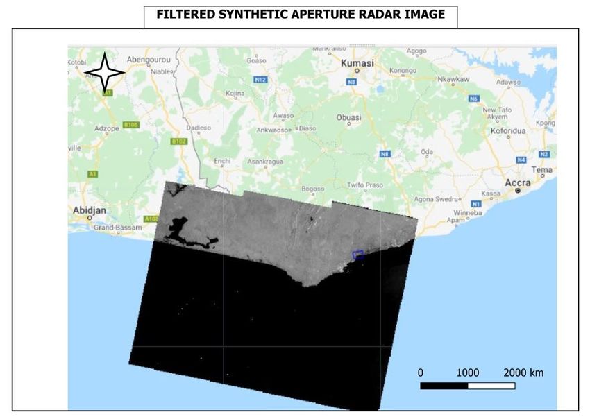
backscatter characteristics of SAR imagery making sure that the selected samples are also within the
Landsat imagery since it will also be used to train the Optical classifier.
In order to run the classifier on the satellite image, the first thing was to pick the training polygons created
earlier and overlay them on the Landsat image. This was done by using the FeatureCollection to extract
reflectance value for each land cover class. Now, the random forest classifier was ‘run’ on both the Optical
and SAR data (Fig. 7) by overlaying the training samples on both the Optical and SAR data. The classifier
was ‘trained’ and ‘run’.
Figure 7: Overlay of Optical and SAR Data
2.3.5 Time Series Comparison
The above process was repeated using ALOS PALSAR 2009 and Landsat 7 image of 2009. However, a
different function to add spectral indices was created because Landsat 7 has different band numbers
from Landsat 8 which also collects images in wider swath. Mangrove area/extent for the two different
time period was calculated using a ‘reduce region’ function in the GEE code editor to calculate the sum of
pixels within the study area that are Mangroves and then convert it to hectares.
2.3.6 Independent Accuracy Assessment
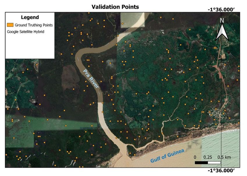
A total of 1553 points were created using the stratified random sampling method (Fig. 8) for the study
site. The accuracy of the classification was assessed using confusion matrix based on the classifier. The
sample points were randomly split for ‘training’ and validation; 80% (1232 points) of the sampling points
were used to ‘train’ the model while 20% (321 points) was used for validation. This was done to remove
any systematic error as a result of using the same pixels to train and validate classifiers (Shi et al., 2016;
Pimple et al., 2018). An independent accuracy assessment was performed in QGIS using the class
accuracy plugin.
Figure 8: Training and Validation Points for the study area
To do this, a variable for the stratified random sample was created by taking the final classification and
using ‘.stratifiedsample’ to create a number of random samples (Barenblitt and Fatoyinbo, 2020b). A
buffer was added to the points so that points with 30m diameter can be visualized and to also reflect the
scale of the imageries. Then, the layers of interest were exported to Google drive for further processing.
3. Results
Image classification was carried out using Random Forest algorithm which is an ensemble tree based
learning algorithm. It creates decision trees that use the pixel values of a data as well as different
variables such as NDVI or different bands of Landsat images to identify different spatial classes by
casting a vote. Several iterations were run using different datasets of SAR, PALSAR, Landsat 7, Landsat 8
as well as a combination of both SAR or PALSAR and optical data with adjustment of different
classification parameters.
Page 8/27
Table 2
                              Mangrove Extent for the Time Period using Different
                                           Classification Scenario
                              Classification Scenarios       Mangrove Extent

                                                             2009 (ha)       2019 (ha)

                              Optical data                   1067.38         1636.81

                              SAR data                       1566.1          1492.2

                              Optical & SAR                  1792.1          1488.53

Three main classification scenarios were established to quantify the extent of mangroves for two-time
period; classification of optical data only, classification of SAR data only, and the third scenario combined
both optical and SAR data (Figs. 9 and 10). The first classification scenario using optical data (Landsat 7
and Landsat 8 showed high performance in terms of the vegetation but fail to pick-up certain features
correctly. The Landsat 8 data performed better than the Landsat 7 data with Mangrove extent of
1067.38ha (Landsat 7) and 1636.81ha (Landsat 8) for 2009 and 2019 respectively (Table 2).

Figure 9: (A) Classification Scenario using Optical data only (Landsat 7); (B) Classification Scenario using
PALSAR data; (C) Classification Scenario using both Optical and PALSAR data

The overall classification accuracy for this scenario is 99.1% and the Kappa Coefficient is 0.797.

                                                Table 3
             Confusion/Error Matrix of Land Cover Classification using Optical Satellite Image
 Classes                  Open           Mangroves       Bare            Vegetation/     Row     User’s
                          Water                          Land                            Total   Accuracy
                                                                         Wetland
                                                                                                 (%)

 Open Water               81             0               0               0               81      100

 Mangroves                0              642             1               4               647     99.2

 Bare Land                0              0               32              0               32      100

 Vegetation/Wetland       0              9               0               936             945     99

 Column Total             81             651             33              940             1705

 Producer’s               100            98.6            96.9            99.5
 Accuracy

 (%)

 Overall Accuracy = 99.18%; Kappa Coefficient = 0.797

                                                   Page 9/27
Table 4
Confusion/Error Matrix of Land Cover Classification using Synthetic Aperture Radar Data
Classes Open Mangroves Bare Vegetation/ Row User’s
Water Land Total Accuracy
Wetland
(%)
Open Water 79 0 2 0 81 97.5
Mangroves 0 521 0 126 647 80.5
Bare Land 2 0 23 7 32 71.9
Vegetation/ 0 119 6 820 945 86.8
Wetland
Column Total 81 640 31 953 1705
Producer’s 97.5 81.4 74.2 86
Accuracy
(%)
Overall Accuracy = 84.6%; Kappa Coefficient = 0.687
Figure 10: (A) Classification Scenario using Optical data only (Landsat 8); (B) Classification Scenario
using SAR data only; (C) Classification Scenario using both Optical and SAR data.
The second classification scenario using SAR data (C-band) did not classify the vegetation units into
much detail despite using the same training samples. However, the PALSAR (L-band) data performed
better than the SAR (C-band) data. The second classification scenario showed Mangrove extent of
1566.1ha (PALSAR L-band) and 1492.2ha (SAR C-band) for 2009 and 2019 respectively.
Page 10/27Table 5
Confusion/Error Matrix of Land Cover Classification using a combination of Optical Satellite Image and
SAR
Classes Open Mangroves Bare Vegetation/ Row User’s
Water Land Total Accuracy
Wetland
(%)
Open Water 81 0 0 0 81 100
Mangroves 0 635 0 12 647 99.2
Bare Land 4 0 28 0 32 100
Vegetation/Wetland 0 3 0 942 945 99
Column Total 85 638 28 954 1705
Producer’s 95.3 99.5 100 98.7
Accuracy
(%)
Overall Accuracy = 98.9%; Kappa Coefficient = 0.828
The overall classification accuracy for this scenario is 84.6% and the Kappa Coefficient is 0.687. The third
classification scenario using a combination of both optical and SAR data achieved the best classification
results as the classes were relatively well distributed with mangroves clustered together close to the water
body. The third classification scenario showed Mangrove extent of 1792.1ha and 1488.53ha for 2009
and 2019 respectively. The overall classification accuracy for this scenario is 98.9% with Kappa
Coefficient of 0.828.
4. Discussion
This study confirms that the combination of Synthetic Aperture Radar data with optical satellite data is
the way forward in mangrove assessment and mapping as recommended by several authors (Attarchi
and Gloaguen, (2014); Ayman et al., 2017; Hu et al., 2020). The Random forest algorithm performed well
to clearly classify the different land cover classes within the area under investigation. The resulting
classification is in agreement with other studies that used random forest for land cover classification
(Ming et al., 2016; Thanh et al., 2020). The outputs of the random forest classification were compared by
overlaying them to visualize some of the differences. The results show that there are differences in all the
three classifications for each time period (2009–2019). For example, the classification using Synthetic
Aperture Radar data indicates that most of the structural aspects of the vegetation were picked up as
compared to when Optical satellite data was used which agrees with the observations in other studies
(Carreiras et al., 2013; Lucas et al., 2014; Nathan et al., 2018). In contrast, Optical satellite image
classification tend to more accurately represent the forest canopy and was able to distinguish between
water bodies from areas of very low vegetation.
Page 11/27The ALOS PALSAR L-Band data was more effective than the Sentinel 1 C-Band SAR data in the
characterization of mangroves probably because of the high penetration capabilities of L-band into
forests canopy. The confusion matrix for SAR image classification alone showed that out of 81 pixels
which were identified as water body, 72 pixels were correctly classified while the confusion matrix for
Optical image alone showed that out of 81 pixels which were identified as water body, all were correctly
classified (Table 3–5). The overall classification accuracy for SAR image alone showed 84% while the
overall accuracy for Optical image alone showed 99.1% and the overall accuracy when both images were
used showed 98.9%. However, the Kappa coefficient value (0.828) shows that the classification using
both Optical and Radar data has better agreement in the observations. The maps produced are suitable
to inform coastal management in the area and the methodology can be reproduced for the entire coastal
zone of Ghana.
5. Conclusion
The destruction of the world’s tropical and sub-tropical mangrove forests is one of the most pressing
environmental disasters of our time. The world may not reach the sustainable development goals without
addressing deforestation and increasing restoration of mangroves as well as other forests. This paper
elaborated on a novel approach to synthesize the relevant database in a spatial framework using Google
Earth Engine platform and random forest algorithm to produce mangrove extent maps. Cloud computing
techniques and machine learning algorithm such as Google Earth Engine as used in this study has shown
the potential for accurate quantification of Mangrove stand as well as various other land uses particularly
for cloud prone areas. This could allow for more accurate estimation of mangrove changes locally,
regionally or globally and to track progress in the sustainable development goals (SDGs).
The combination of optical satellite data alongside synthetic aperture radar and random forest algorithm
could be valuable for mapping changes in mangrove ecosystems and their surroundings to fill knowledge
gaps essential for Mangrove management and conservation. Overall, there is a significant (16%) decadal
decrease of mangrove extent in the study location which presents the need for conservation and proper
monitoring and management. This would require a deliberate management plan encompassing current
and alternative livelihood strategies, sustainable resource management schemes and sustained
sensitization of the people about mangrove services and their value under climate change, beyond
providing the immediate needs of the community. There should be continuous re-planting of Mangrove
propagules in areas where there has been degradation.
Although our model estimates mangrove extent fairly well, the main limitation to this study is the lack of
up to date data e.g. 2020 data as at the time of this analyses.
Abbreviations
ALOS – Advanced Land Observation Satellite
Page 12/27ASTER – Advanced Space-borne Thermal Emission and Reflection Radiometer
DEM – Digital Elevation Model
ESA - European Space Agency
ETM+ - Enhanced Thematic Mapper
GCVI - Green chlorophyll vegetation index
GDEM – Global Digital Elevation Model
GEE – Google Earth Engine
GMTED – Global Multi-resolution Terrain Elevation Data
HH - single co-polarization, horizontal transmit/horizontal receive
NASA - National Aeronautics and Space Administration
NDMI - Normalized difference moisture index
NDVI - Normalized difference vegetation index
NDWI - Modified normalized difference water index
NED – National Elevation Data (US Geological Survey)
OLI/TIRS - Operational Land Imager/Thermal Infrared Sensor
PALSAR – Phase Array L-band Synthetic Aperture Radar
SAR – Synthetic Aperture Radar
SDGs – Sustainable Development Goals
SR - Simple ratio
SRTM – Shuttle Radar Topographic Mission
VV- single co-polarization, vertical transmit/vertical receive
Declarations
Ethics approval and consent to participate
Not applicable
Page 13/27Consent for publication
Not applicable
Availability of data and materials
The datasets generated and/or analyzed during the current study are available in Google Earth Engine
database. The Java codes used for this study can be found at
https://code.earthengine.google.com/a2400e2ce048914ccf1b16aba2702951
Competing interests
The authors declare no competing interests
Funding
This work is part of the corresponding author’s PhD research which is funded by the World Bank ACE
impact project III in collaboration with the government of Ghana.
Authors' contributions
Conceptualization, D.A., M.M and D.B.A.; methodology, D.A., M.M and D.B.A.; software, D.A.; validation,
D.A.; writing—original draft preparation, D.A.; writing—review and editing, D.A., M.M and D.B.A. All authors
have read and agreed to the published this manuscript.
Acknowledgements
The authors wish to thank the Management of Africa Center of Excellence in Coastal Resilience (ACECoR)
for attracting the funds and bringing us on board via scholarship. We also acknowledge the role of Mr.
Daniel Doku Nii Nortey during reconnaissance survey and field assistance.
References
Alongi D M (2012) Carbon sequestration in mangrove forests. Carbon Management 3: 313-322.
Attarchi S, Gloaguen R (2014) Classifying Complex Mountainous Forests with L-Band SAR and Landsat
Data Integration: A Comparison among Different Machine Learning Methods in the Hyrcanian
Forest. Remote Sens. 6: 3624-3647.
Page 14/27Ayman AH, Olena D, Islam AE, Gunter M (2017) Integration of SAR and Optical Remote Sensing data for
mapping of mangroves extents. In: From Science to Society: The Bridge provided by Environmental
Informatics. (Ed. Benoît Otjacques, Patrik Hitzelberger, Stefan Naumann, Volker Wohlgemuth) Germany:
Shaker Verlag GmbH, p. 1 - 8
Barenblitt A, Fatoyinbo L (2020a) Intro to SDG 6.6 and Remote Sensing Techniques for Mangroves.
NASA’s Applied Remote Sensing Training Program
Barenblitt A, Fatoyinbo L (2020b) Mangrove Extent Mapping and Time Series. NASA’s Applied Remote
Sensing Training Program
Blasco F, Aizpuru M, Besnehard J (2019) Mangroves, Ecology. Encyclopedia of Coastal Science, Springer
Nature Switzerland AG Finkl. W. Charls and Makowski Christopher (eds.) https://doi.org/10.1007/978-3-
319-93806-6
Breithaupt J L, Smoak J M, Smith T J, Sanders C J, Hoare A (2012) Organic carbon burial rates in
mangrove sediments: Strengthening the global budget. Global Biogeochemical Cycles 26(3).
Carreiras JMB, Melo JM, Vasconcelos MJ (2013) Estimating the above-ground biomass in Miombo
Savanna woodlands (Mozambique, East Africa) using L-band synthetic aperture radar data. Remote Sens
5(4):1524–1548
Coastal Resources Center / Friends of the Nation (2010). Report on Characterization of Coastal
Communities and Shoreline Environments in the Western Region of Ghana. Integrated Coastal and
Fisheries Governance Initiative for the Western Region of Ghana. Coastal Resources Center, University of
Rhode Island, 425 pages.
De Santiago FF, Kovacs JM, Lafrance P (2013) An object-oriented classification method for mapping
mangroves in Guinea, West Africa, using multipolarized ALOS PALSAR L-band data. Int. J. Remote Sens.,
34: 563–586.
Ellison A, Farnsworth E, Moore G (2015) Rhizophora Mangle. The IUCN Red List of Threatened Species.
Erika P, Amber M, Juan L, Torres P, Sean M (2020) Forest Mapping and Monitoring with SAR Data: Time
Series Analysis. NASA’s Applied Remote Sensing Training Program
FAO (2007) The World's Mangroves 1980-2005. FAO Forestry Paper Rome, Forest Resources Division: 77.
Farr, T.G., Rosen, P.A., Caro, E., Crippen, R., Duren, R., Hensley, S., Kobrick, M., Paller, M., Rodriguez, E., Roth,
L., Seal, D., Shaffer, S., Shimada, J., Umland, J., Werner, M., Oskin, M., Burbank, D., and Alsdorf, D.E., 2007,
The shuttle radar topography mission: Reviews of Geophysics, v. 45, no. 2, RG2004,
at https://doi.org/10.1029/2005RG000183.
Page 15/27Friends of the Nation (2014), Assessment of flora and fauna of ecological and socioeconomic
significance within the Anlo Beach Wetland Complex for improved management and livelihood outcomes,
Parks and Gardens, Adiembra, 60 pp.
Gedan KB, Kirwan ML, Wolanski E, Barbier EB, Silliman BR (2011) The present and future role of coastal
wetland vegetation in protecting shorelines: Answering recent challenges to the paradigm. Clim. Chang.,
106: 7–29.
Giri C, Ochieng E, Tieszen LL, Zhu Z, Singh A, Loveland T, Masek J, Duke N (2011) Status and distribution
of mangrove forests of the world using earth observation satellite data. Glob. Ecol. Biogeogr. 20: 154–
159.
Hansen MC, Potapov PV, Moore R, Hancher M, Turubanova SA, Tyukavina A, Thau D, Stehman SV, Goetz
SJ, Loveland TR (2013) High-resolution global maps of 21st century forest cover change. Science, 342:
850–853.
Hu T, YingYZ, Yanjun S, Yi Z, Guanghui L, Qinghua G (2020) Mapping the Global Mangrove Forest
Aboveground Biomass Using Multisource Remote Sensing Data. Remote Sens. 12: 1690.
doi:10.3390/rs12101690
Kovacs JM, de Santiago FF, Bastien J, Lafrance P (2010) An Assessment of Mangroves in Guinea, West
Africa, Using a Field and Remote Sensing Based Approach. Wetlands, 30:773–782.
Kuenzer, C, Tuan VQ (2013) Assessing the ecosystem services value of Can Gio Mangrove Biosphere
Reserve: Combining earth-observation- and household-survey-based analyses. Appl. Geogr., 45: 167–184.
Lavalle M, Wright T (2009) Absolute radiometric and polarimetric calibration of ALOS PALSAR products.
Available online: https://earth.esa.int/eogateway/documents/20142/37627/ ALOS-PALSAR-calibration-
products-ADEN.pdf?category=Document+library (accessed on 10 December 2020)
Lee SY, Primavera JH, Dahdouh-Guebas F, McKee K, Bosire JO, Cannicci S, Diele K, Fromard F, Koedam N,
Marchand C (2014) Ecological role and services of tropical mangrove ecosystems: A reassessment:
Reassessment of mangrove ecosystem services. Glob. Ecol. Biogeogr. 23: 726–743.
Lucas R, Rebelo L, Fatoyinbo L, Rosenqvist A, Itoh T, Shimada M, Simard M, Pedro WS, Nathan T, Carl T,
Arnon A, Joao C, Lammert H (2014) Contribution of L-band SAR to systematic global mangrove
monitoring. Marine and Freshwater Research, 65:589–603 http://dx.doi.org/10.1071/MF13177
Mayaux P, Holmgren P, Achard F, Eva H, Stibig HJ, Branthomme A (2005) Tropical forest cover change in
the 1990s and options for future monitoring. Philosophical Transactions of the Royal Society of London
B: Biological Sciences 360(1454): 373-384.
Page 16/27Ming D, Zhou T, Wang M, Tian T, (2016) Land cover classification using random forest with genetic
algorithm-based parameter optimization, J. Appl. Remote Sens. 10(3), 035021. doi:
10.1117/1.JRS.10.035021
Miththapala, S (2008) Mangroves. Coastal Ecosystems. Colombo Sri Lanka, Ecosystems and Livelihoods
Group Asia. 2.
Mondal P, Trzaska S, de Sherbinin A (2018) Landsat-Derived Estimates of Mangrove Extents in the Sierra
Leone Coastal Landscape Complex during 1990–2016. Sensors, 18:12.
Nathan T, Peter B, Richard L, Andy H, Ake R, Temilola F (2018) Mapping Mangrove Extent and Change: A
Globally Applicable Approach Remote Sens., 10:1466. doi:10.3390/rs10091466
Nortey DDN, Aheto DW, John B, Fredrick EJ, Asare NK (2016) Comparative Assessment of Mangrove
Biomass and Fish Assemblages in an Urban and Rural Mangrove Wetlands in Ghana. Society of Wetland
Scientists. DOI 10.1007/s13157-016-0783-2
Omo-Irabor OO, Olobaniyi SB, Akunna J, Venus V, Maina JM, Paradzayi C (2011) Mangrove vulnerability
modelling in parts of Western Niger Delta, Nigeria using satellite images, GIS techniques and Spatial
Multi-Criteria Analysis (SMCA). Environ. Monit. Assess, 178: 39–51.
Otero V, Quisthoudt K, Koedam N, Dahdouh-Guebas F (2016) Mangroves at Their Limits: Detection and
Area Estimation of Mangroves along the Sahara Desert Coast. Remote Sens., 8: 512.
Pimple U, Simonetti D, Sitthi A, Pungkul S, Leadprathom K, Skupek H, Som-ard J, Gond V, Towprayoon S
(2018) Google Earth Engine Based Three Decadal Landsat Imagery Analysis for Mapping of Mangrove
Forests and Its Surroundings in the Trat Province of Thailand. Journal of Computer and Communications,
6: 247-264. https://doi.org/10.4236/jcc.2018.61025
Salami AT, Akinyede J, de Gier A (2010) A preliminary assessment of NigeriaSat-1 for sustainable
mangrove forest monitoring. Int. J. Appl. Earth Obs. Geoinf., 12: S18–S22.
Shi T, Jue L, Zhongwen H, Huizeng L, Junjie W, Guofeng W (2016) New spectral metrics for mangrove
forest identification, Remote Sensing Letters, 7:(9) 885-894. DOI: 10.1080/2150704X.2016.1195935
Son NT, Chen CF, Chang NB, Chen CR, Chang LY, Thanh BX (2015) Mangrove Mapping and Change
Detection in Ca Mau Peninsula, Vietnam, Using Landsat Data and Object-Based Image Analysis. IEEE
Journal of Selected Topics in Applied Earth Observations and Remote Sensing, 8: 503-510.
https://doi.org/10.1109/JSTARS.2014.2360691
Thanh NP, Verena K, Lukas WL (2020) Land Cover Classification using Google Earth Engine and Random
Forest Classifier-The Role of Image Composition. Remote Sens., 12: 2411.
https://doi.org/10.3390/rs12152411
Page 17/27World Mangrove Network (2012). Western Indian Ocean Mangrove Network/United States Forest Service
Workshop Report, Maputo, Mozambique.
Zhang C, Kovacs JM, Liu Y, Flores-Verdugo F, Flores-de-Santiago F (2014) Separating Mangrove Species
and Conditions Using Laboratory Hyperspectral Data: A Case Study of a Degraded Mangrove Forest of
the Mexican Pacific. Remote Sensing, 6: 11673-11688. https://doi.org/10.3390/rs61211673
Figures
Figure 1
Map of Study Location. Note: The designations employed and the presentation of the material on this
map do not imply the expression of any opinion whatsoever on the part of Research Square concerning
the legal status of any country, territory, city or area or of its authorities, or concerning the delimitation of
its frontiers or boundaries. This map has been provided by the authors.
Page 18/27Figure 2
Key concepts related to sustainable development and links to the most relevant sustainable development
goals, targets, indicators and series. Note: The designations employed and the presentation of the
material on this map do not imply the expression of any opinion whatsoever on the part of Research
Square concerning the legal status of any country, territory, city or area or of its authorities, or concerning
the delimitation of its frontiers or boundaries. This map has been provided by the authors.
Page 19/27Figure 3
Cloud Free Landsat 8 Imagery. Note: The designations employed and the presentation of the material on
this map do not imply the expression of any opinion whatsoever on the part of Research Square
concerning the legal status of any country, territory, city or area or of its authorities, or concerning the
delimitation of its frontiers or boundaries. This map has been provided by the authors.
Page 20/27Figure 4
False Color Composite of Landsat Image Clipped to Study Area. Note: The designations employed and
the presentation of the material on this map do not imply the expression of any opinion whatsoever on
the part of Research Square concerning the legal status of any country, territory, city or area or of its
authorities, or concerning the delimitation of its frontiers or boundaries. This map has been provided by
the authors.
Page 21/27Figure 5
Filtered Synthetic Aperture Radar Image. Note: The designations employed and the presentation of the
material on this map do not imply the expression of any opinion whatsoever on the part of Research
Square concerning the legal status of any country, territory, city or area or of its authorities, or concerning
the delimitation of its frontiers or boundaries. This map has been provided by the authors.
Page 22/27Figure 6
Iteration Process for Random Forest Model
Page 23/27Figure 7
Overlay of Optical and SAR Data. Note: The designations employed and the presentation of the material
on this map do not imply the expression of any opinion whatsoever on the part of Research Square
concerning the legal status of any country, territory, city or area or of its authorities, or concerning the
delimitation of its frontiers or boundaries. This map has been provided by the authors.
Page 24/27Figure 8
Training and Validation Points for the study area. Note: The designations employed and the presentation
of the material on this map do not imply the expression of any opinion whatsoever on the part of
Research Square concerning the legal status of any country, territory, city or area or of its authorities, or
concerning the delimitation of its frontiers or boundaries. This map has been provided by the authors.
Page 25/27Figure 9
(A) Classification Scenario using Optical data only (Landsat 7); (B) Classification Scenario using PALSAR
data; (C) Classification Scenario using both Optical and PALSAR data The overall classification accuracy
for this scenario is 99.1% and the Kappa Coefficient is 0.797. Note: The designations employed and the
presentation of the material on this map do not imply the expression of any opinion whatsoever on the
part of Research Square concerning the legal status of any country, territory, city or area or of its
authorities, or concerning the delimitation of its frontiers or boundaries. This map has been provided by
the authors.
Page 26/27Figure 10
(A) Classification Scenario using Optical data only (Landsat 8); (B) Classification Scenario using SAR
data only; (C) Classification Scenario using both Optical and SAR data. Note: The designations employed
and the presentation of the material on this map do not imply the expression of any opinion whatsoever
on the part of Research Square concerning the legal status of any country, territory, city or area or of its
authorities, or concerning the delimitation of its frontiers or boundaries. This map has been provided by
the authors.
Page 27/27You can also read