Non-Mergeable Sketching for Cardinality Estimation - DROPS
←
→
Page content transcription
If your browser does not render page correctly, please read the page content below
Non-Mergeable Sketching for Cardinality
Estimation
Seth Pettie #
University of Michigan, Ann Arbor, MI, USA
Dingyu Wang          #
University of Michigan, Ann Arbor, MI, USA
Longhui Yin #
Tsinghua University, Beijing, China

          Abstract
Cardinality estimation is perhaps the simplest non-trivial statistical problem that can be solved via
sketching. Industrially-deployed sketches like HyperLogLog, MinHash, and PCSA are mergeable, which
means that large data sets can be sketched in a distributed environment, and then merged into a
single sketch of the whole data set. In the last decade a variety of sketches have been developed that
are non-mergeable, but attractive for other reasons. They are simpler, their cardinality estimates are
strictly unbiased, and they have substantially lower variance.
    We evaluate sketching schemes on a reasonably level playing field, in terms of their memory-
variance productp(MVP). E.g., a sketch that occupies 5m bits and whose relative variance is 2/m
(standard error 2/m) has an MVP of 10. Our contributions are as follows.

        Cohen [14] and Ting [35] independently discovered what we call the Martingale transform for
        converting a mergeable sketch into a non-mergeable sketch. We present a simpler way to analyze
        the limiting MVP of Martingale-type sketches.
        Pettie and Wang proved that the Fishmonger sketch [31] has the best MVP, H0 /I0 ≈ 1.98, among
        a class of mergeable sketches called “linearizable” sketches. (H0 and I0 are precisely defined
        constants.) We prove that the Martingale transform is optimal in the non-mergeable world, and
        that Martingale Fishmonger in particular is optimal among linearizable sketches, with an MVP of
        H0 /2 ≈ 1.63. E.g., this is circumstantial evidence that to achieve 1% standard error, we cannot
        do better than a 2 kilobyte sketch.
        Martingale Fishmonger is neither simple nor practical. We develop a new mergeable sketch called
        Curtain that strikes a nice balance between simplicity and efficiency, and prove that Martingale
        Curtain has limiting MVP ≈ 2.31. It can be updated with O(1) memory accesses and it has lower
        empirical variance than Martingale LogLog, a practical non-mergeable version of HyperLogLog.
2012 ACM Subject Classification Theory of computation → Sketching and sampling
Keywords and phrases Cardinality Estimation, Sketching
Digital Object Identifier 10.4230/LIPIcs.ICALP.2021.104
Category Track A: Algorithms, Complexity and Games
Related Version Full Version: https://arxiv.org/abs/2008.08739
Funding This work was supported by NSF grants CCF-1637546 and CCF-1815316.

    1      Introduction
Cardinality estimation 1 is a fundamental problem in streaming and sketching with diverse
applications in databases [12, 21], network monitoring [5, 8, 39, 11], nearest neighbor
search [33], caching [37], and genomics [30, 17, 38, 2]. In the sequential setting of this
problem, we receive the elements of a multiset A = {a1 , a2 , . . . , aN } one at a time. We

1
    (aka F0 estimation or Distinct Elements)
            © Seth Pettie, Dingyu Wang, and Longhui Yin;
            licensed under Creative Commons License CC-BY 4.0
                                                                                                      EA
                                                                                                      TC S

48th International Colloquium on Automata, Languages, and Programming (ICALP 2021).
Editors: Nikhil Bansal, Emanuela Merelli, and James Worrell; Article No. 104; pp. 104:1–104:20
                   Leibniz International Proceedings in Informatics
                   Schloss Dagstuhl – Leibniz-Zentrum für Informatik, Dagstuhl Publishing, Germany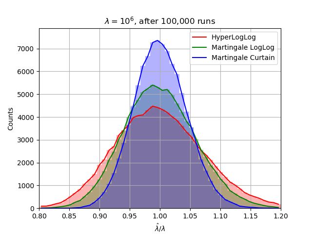
104:2   Non-Mergeable Sketching for Cardinality Estimation

        maintain a small sketch S of the elements seen so far, such that the true cardinality λ = |A|
        is estimated by some λ̂(S). The distributed setting is similar, except that A is partitioned
        arbitrarily among several machines, the shares being sketched separately and combined into
        a sketch of A. Only mergeable sketches are deployed in distributed settings; see Definition 2
        below.

        ▶ Definition 1. In the random oracle model A ⊆ [U ] and we have oracle access to
        a uniformly random permutation h : [U ] → [U ] (or a uniformly random hash function
        h : [U ] → [0, 1]). In the standard model we can generate random bits as necessary, but
        must explicitly store any hash functions in the sketch.

        ▶ Definition 2. Suppose A(1) , A(2) are multisets such that A = A(1) ∪ A(2) . A sketching
        scheme is mergeable if, whenever, A(1) , A(2) are sketched as S (1) , S (2) (using the same
        random oracle h or the same source of random bits in the standard model), the sketch
        S of A can be computed from S (1) , S (2) alone.

             Standard model sketches [1, 3, 4, 6, 22, 27] usually make an (ϵ, δ)-guarantee, i.e.,

             Pr λ̂ ̸∈ [(1 − ϵ)λ, (1 + ϵ)λ] < δ.

        The state-of-the-art standard model sketch [6, 27] uses O(ϵ−2 log δ −1 + log U ) bits, which
        is optimal at this level of specificity, as it meets the space lower bounds of Ω(log U ), Ω(ϵ−2 )
        (when δ = Θ(1)), and Ω(ϵ−2 log δ −1 ) [1, 25, 26]. However, the leading constants hidden
        by [6, 27] are quite large.
            In the random oracle model the cardinality estimate λ̂ typically has negligible bias,
                       expressed in terms of the relative variance λ−2 · Var(λ̂ | λ) or relative standard
        and errors are q
        deviation λ−1 Var(λ̂ | λ), also called the standard error. Sketches that use Ω(m) bits
        typically have relative variances of O(1/m). Thus, the most natural way to measure the
        quality of the sketching scheme itself is to look at its limiting memory-variance product
        (MVP), i.e., the product of its memory and variance as m → ∞.
            Until about a decade ago, all standard/random oracle sketches were mergeable,
        and suitable to both distributed and sequential applications. For reasons that are not clear
        to us, the idea of non-mergeable sketching was discovered independently by multiple
        groups [10, 24, 14, 35] at about the same time, and quite late in the 40-year history of
        cardinality estimation. Chen, Cao, Shepp, and Nguyen [10] invented the S-Bitmap in
        2011, followed by Helmi, Lumbroso, Martínez, and Viola’s[24] Recordinality in 2012. In 2014
        Cohen [14] and Ting [35] independently invented what we call the Martingale transform, which
        is a simple, mechanical way to transform any mergeable sketch into a (better) non-mergeable
        sketch.2
            In a companion paper [31], we analyzed the MVPs of mergeable sketches under the
        assumption that the sketch was compressed to its entropy bound. Fishmonger (an entropy
        compressed variant of PCSA with a different estimator function) was shown to have MVP =
        H0 /I0 ≈ 1.98, where
                                   ∞
                                                                         and I0 = ζ(2) = π 2 /6.
                                   X
                          −1
             H0 = (ln 2)       +         k −1 log2 (1 + 1/k)
                                   k=1

        2
            Cohen [14] called these Historical Inverse Probability (HIP) sketches and Ting [35] applied the prefix
            Streaming to emphasize that they can be used in the single-stream setting, not the distributed setting.
S. Pettie, D. Wang, and L. Yin 104:3
Furthermore, H0 /I0 was shown to be the minimum MVP among linearizable sketches, a
subset of mergeable sketches that includes all the popular sketches (HyperLogLog, PCSA,
MinHash, etc.).
Our aim in this paper is to build a useful framework for designing and analyzing non-
mergeable sketching schemes, and, following [31], to develop a theory of space-variance
optimality in the non-mergeable world. We work in the random oracle model. Our
results are as follows.
Although the Martingale transform itself is simple, analyzing the variance of these sketches
is not. For example, Cohen p [14] and Ting [35]√estimated the standard error of Martingale
LogLog to be about ≈ p3/(4m) ≈ 0.866/ m and about ≈ 1/(2αm m), respectively,
√
where the latter tends to ln 2/m ≈ 0.8326/ m as m → ∞.3 We give a general method
for determining the limiting relative variance of Martingale sketches that is strongly
influenced by Ting’s perspective.
What is the most efficient (smallest MVP) non-mergeable sketch for cardinality estimation?
The best Martingale sketches perform better than the ad hoc non-mergeable S-Bitmap and
Recordinality, but perhaps there is a completely different, better way to systematically
build non-mergeable sketches. We prove that up to some natural assumptions4 the best
non-mergeable sketch is a Martingale X sketch, for some X. Furthermore, we prove that
Martingale Fishmonger, having MVP of H0 /2 ≈ 1.63, is optimal among all Martingale
X sketches, where X is linearizable. This provides some circumstantial evidence that
Martingale Fishmonger is optimal, and that if we want, say, 1% standard error, we need
to use a H0 /2 · (0.01)−2 -bit sketch, ≈ 2 kilobytes.
Martingale Fishmonger has an attractive MVP, but it is slow and cumbersome to implement.
We propose a new mergeable sketch called Curtain that is “naturally” space efficient and
easy to update in O(1) memory accesses, and prove that Martingale Curtain has a limiting
MVP ≈ 2.31.
1.1 Prior Work: Mergeable Sketches
Let Si be the state of the sketch after processing (a1 , . . . , ai ).
The state of the PCSA sketch [20] is a 2D matrix S ∈ {0, 1}m×log U and the hash function
h : [U ] → [m] × Z+ produces two indices: h(a) = (j, k) with probability m−1 2−k . Si (j, k) = 1
iff ∃i′ ∈ [i].h(ai′ ) = (j, k). Flajolet and Martin [20] proved that a certain estimator has
√
standard error 0.78/ m, making the MVP around (0.78)2 log U ≈ 0.6 log U .
Durand and Flajolet’s LogLog sketch [16] consists of m counters. It interprets h exactly as
in PCSA, and sets Si (j) = k iff k is maximum suchPthat ∃i′ ∈ [i].h(ai′ ) = (j, k). Durand and
m−1 S(j) √
Flajolet’s estimator is of the form λ̂(S) ∝ m2 j and has standard error ≈ 1.3/ m.
Flajolet, Fusy, Gandouet, and Meunier’s HyperLogLog [19] is the same sketch but with the
estimator λ̂(S) ∝ m2 ( j 2−S(j) )−1 . They proved that it has standard error tending to
P
√
≈ 1.04/ m. As the space is m log log U bits, the MVP is ≈ 1.08 log log U .
The MinCount sketch (aka MinHash or Bottom-m [13, 15, 7]) stores the smallest m hash
values, which we assume requires log U bits each. Using an appropriate estimator [23, 9, 29],
√
the standard error is 1/ m and MVP = log U .
3
R∞ 2+u
m −1
Here αm = m 0 log2 1+u du is the coefficient of Flajolet et al.’s HyperLogLog estimator.
4
(the sketch is insensitive to duplicates, and the estimator is unbiased)
ICALP 2021104:4 Non-Mergeable Sketching for Cardinality Estimation
It is straightforward to see that the entropy of PCSA and LogLog are both Θ(m).
Scheuermann and Mauve [34] experimented with entropy compressed versions of PCSA and
HyperLogLog and found PCSA to be slightly superior. Rather than use the given estimators
of [20, 19, 16], Lang [28] used Maximum Likelihood-type Estimators and found entropy-
compressed PCSA to be significantly better than entropy-compressed LogLog (with MLE
estimators). Pettie and Wang [31] defined the Fisher-Shannon (Fish)5 number of a sketch
as the ratio of its Shannon entropy (controlling its entropy-compressed size) to its Fisher
information (controlling the variance of a statistically efficient estimator), and proved that
the Fish-number of any base-q PCSA is H0 /I0 , and that the Fish-number of base-q LogLog is
worse, but tends to H0 /I0 in the limit as q → ∞. (The constants H0 , I0 were defined earlier.)
Table 1 A selection of results on composable sketches (top) and non-composable Martingale
sketches (bottom) in terms of their limiting memory-variance product (MVP). Logarithms are
base 2.
Mergeable Sketch Limiting MVP Notes
PCSA [20] .6 log U ≈ 38.9 For U = 264
LogLog [16] 1.69 log log U ≈ 10.11 For U = 264
MinCount [23, 9, 29] log U = 64 For U = 264
HyperLogLog [19] 1.08 log log U ≈ 6.48 For U = 264
Fishmonger [31] H0 /I0 ≈ 1.98
Non-Mergeable Sketch
S-Bitmap [10] O(log2 (U/m))
Recordinality [24] O(log(λ/m) log U )
Martingale PCSA new 0.35 log U ≈ 22.4 For U = 264
Martingale LogLog [14, 35] 0.69 log log U ≈ 4.16 For U = 264
Martingale MinCount [14, 35] 0.5 log U = 32 For U = 264
log2 (1+1/k)
H0 = (ln 2)−1 + k≥1
P
Martingale Fishmonger new H0 /2 ≈ 1.63 k
Martingale Curtain new ≈ 2.31 Theorem 4 with (q, a, h) = (2.91, 2, 1)
Non-Mergeable Lower Bound
Martingale X new ≥ H0 /2 X is a linearizable sketch
1.2 Prior Work: Non-Mergeable Sketches
Chen, Cao, Shepp, and Nguyen’s S-Bitmap [10] consists of a bit string S ∈ {0, 1}m and m
known constants 0 ≤ τ0 < τ1 < · · · < τm−1 < 1. It interprets h(a) = (j, ρ) ∈ [m] × [0, 1] as
an index j and real ρ and when processing a, sets S(j) ← 1 iff ρ > τHammingWeight(S) . One
may confirm that S is insensitive to duplicates in the stream A, but its state depends on
the order in which A is scanned. By setting the τ -thresholds and estimator properly, the
√
standard error is ≈ ln(eU/m)/(2 m) and MVP = O(log2 (U/m)).
Recordinality [24] is based on MinCount; it stores (S, cnt), where S is the m smallest hash
p that S has changed. The estimator looks
values encountered and cnt is the number of times
only at cnt, not S, and has standard error ≈ ln(λ/em)/m and MVP = O(log(λ/m) log U ).
5
Fish is essentially the same as MVP, under the assumption that the sketch state is compressed to its
entropy.S. Pettie, D. Wang, and L. Yin 104:5
Cohen [14] and Ting [35] independently described how to turn any sketch into a non-
mergeable sketch using what we call the Martingale transform. Let Si be the state of the
original sketch after seeing (a1 , . . . , ai ) and Pi+1 = Pr(Si+1 ̸= Si | Si , ai+1 ̸∈ {a1 , . . . , ai })
be the probability that it changes state upon seeing a new element ai+1 .6 The state of the
Martingale sketch is (Si , λ̂i ). Upon processing ai+1 it becomes (Si+1 , λ̂i+1 ), where
r z
−1
λ̂i+1 = λ̂i + Pi+1 · Si+1 ̸= Si .
r z
Here E is the indicator variable for the event E. We assume the original sketch is insensitive
to duplicates, so
(
λ̂i when ai+1 ∈ {a1 , . . . , ai } (and hence Si+1 = Si )
E(λ̂i+1 ) =
λ̂i + 1 when ai+1 ̸∈ {a1 , . . . , ai }.
Thus, with λ̂0 = λ0 = 0, λ̂i is an unbiased estimator of the true cardinality λi = |{a1 , . . . , ai }|
and (λ̂i − λi )i is a martingale. The Martingale-transformed sketch requires the same space,
plus just log U bits to store the estimate λ̂.
Cohen and Ting [14, 35] both proved that Martingale MinCount has standard error
√
1/(2 m) and MVP = (log U )/2. They gave different estimates for the p standard error of
Martingale LogLog. Ting’s estimate is quite accurate, and tends to ln 2/m as m → ∞,
giving it an MVP = ln 2 log log U ≈ 0.69 log log U .
▶ Remark 3. We call Martingale sketches non-mergeable because, in a distributed environment,
there is no obvious way to merge the cardinality estimates (λ̂). On the other hand, Ting [36]
has shown that if (S A , λ̂A ) and (S B , λ̂B ) are Martingale MinCount sketches obtained by
sequentially processing A and B, that λ̂A , λ̂B carry useful information for estimating |A ∪ B|
and |A ∩ B| beyond that contained in S A , S B .
1.3 The Dartboard Model
The dartboard model [31] is useful for describing cardinality sketches with a single, uniform
language. The dartboard model is essentially the same as Ting’s [35] area cutting process,
but with a specific, discrete cell partition and state space fixed in advance.
The dartboard is the unit square [0, 1]2 , partitioned into a set C = {c0 , . . . , c|C|−1 } of cells
of various sizes. Every cell may be either occupied or unoccupied; the state is the set of
occupied cells and the state space some S ⊆ 2C .
We process a stream of elements one by one; when a new element is encountered we
throw a dart uniformly at random at the dartboard and update the state in response. The
relationship between the state and the dart distribution satisfies two rules:
(R1) Every cell with at least one dart is occupied; occupied cells may contain no darts.
(R2) If a dart lands in an occupied cell, the state does not change.
As a consequence of (R1) and (R2), if a dart lands in an empty cell the state must change,
and occupied cells may never become unoccupied. Dart throwing is merely an intuitive way
of visualizing the hash function. Base-q PCSA and LogLog use the same cell partition but
with different state spaces; see Figure 1.
6
These probabilities are over the choice of h(ai+1 ), which, in the random oracle model, is independent
of all other hash values.
ICALP 2021104:6 Non-Mergeable Sketching for Cardinality Estimation
...
...
(a) (b) (c)
Figure 1 The unit square is partitioned into m columns. Each column is partitioned into cells.
Cell j covers the vertical interval [q −(j+1) , q −j ). (b) The state of a PCSA sketch records precisely
which cells contain a dart (gray); all others are empty (yellow). (c) The state of the corresponding
LogLog sketch.
It was observed [31] that the dartboard model includes all mergeable sketches, and
some non-mergeable ones like S-Bitmap. Recordinality and the Martingale sketches obey
rules (R1),(R2) but are not strictly dartboard sketches as they maintain some small state
information (cnt or λ̂) outside of the set of occupied cells. Nonetheless, it is useful to speak
of the dartboard part of their state information.
1.4 Linearizable Sketches
The lower bound of [31] applies to linearizable sketches, a subset of mergeable sketches. A
sketch is called linearizable if it is possible to encode the occupied/unoccupied status of its
cells in some fixed linear order (c0 , . . . , cC−1 ), so whether ci is occupied only depends on
the status of c0 , . . . , ci−1 and whether ci has been hit by a dart. (Thus, it is independent of
ci+1 , . . . , cC−1 .) Specifically, let Yi , Zi be the indicators for whether ci is occupied, and has
been hit by a dart, respectively, and Yi = (Y0 , . . . , Yi ). The state of the sketch is YC−1 ; it is
called linearizable if there is some monotone function ϕ : {0, 1}∗ → {0, 1} such that
Yi = Zi ∨ ϕ(Yi−1 ).
I.e., if ϕ(Yi−1 ) = 1, ci is forced to be occupied and the state is forever independent of Zi .
PCSA-type sketches [20, 18] are linearizable, as are (Hyper)LogLog [19, 16], and all
MinCount, MinHash, and Bottom-m type sketches [13, 7, 23, 9, 29]. It is very easy to engineer
non-linearizable sketches; see [31]. The open problem is whether this is ever a good idea in
terms of memory-variance performance.
1.5 Organization
In Section 2 we introduce the Curtain sketch, which is a linearizable (hence mergeable)
sketch in the dartboard model. In Section 3 we prove some general theorems on the bias
and asymptotic relative variance of Martingale-type sketches, and in Section 4 we apply
this framework to bound the limiting MVP of Martingale PCSA, Martingale Fishmonger, and
Martingale Curtain.
In Section 5 we prove some results on the optimality of the Martingale transform itself,
and that Martingale Fishmonger has the lowest variance among those based on linearizable
sketches.S. Pettie, D. Wang, and L. Yin 104:7
Section 6 presents some experimental findings that demonstrate that the conclusions
drawn from the asymptotic analysis of Martingale sketches are extremely accurate in the
pre-asymptotic regime as well, and that Martingale Curtain has lower variance than Martingale
LogLog.
All the missing proofs can be found in the full version [32].
2 The Curtain Sketch
Design Philosophy
Our goal is to strike a nice balance between the simplicity and time-efficiency of (Hyper)LogLog,
and the superior information-theoretic efficiency of PCSA, which can only be fully realized
under extreme (and time-inefficient) compression to its entropy bound [31, 28]. Informally,
if we are dedicating at least 1 bit to encode the status of a cell, the best cells to encode
have mass Θ(λ−1 ) and we should design a sketch that maximizes the number of such cells
encoded.
We assume the dartboard is partitioned into m columns; define Cell(j, i) to be the cell in
column i covering the vertical interval [q −(j+1) , q −j ). In a PCSA sketch, the occupied cells
are precisely those with at least one dart. In LogLog, the occupied cells in each column are
contiguous, extending to the highest cell containing a dart. In Figure 1, cells are drawn with
uniform sizes for clarity.
Consider the vector v = (g0 , g1 , . . . , gm−1 ) where Cell(gi , i) is the highest occupied cell in
LogLog/PCSA. The curtain of v w.r.t. allowable offsets O is a vector vcurt = (ĝ0 , ĝ1 , . . . , ĝm−1 )
such that (i) ∀i ∈ [1, m−1]. ĝi − ĝi−1 ∈ O, and (ii) vcurt is the minimal such vector dominating
v, i.e., ∀i. ĝi ≥ gi . Although we have described vcurt as a function of v, it is clearly possible
to maintain vcurt as darts are thrown, without knowing v.
We have an interest in |O| being a power of 2 so that curtain vectors may be encoded
efficiently, as a series of offsets. On the other hand, it is most efficient if O is symmetric
around zero. For these reasons, we use a base-q “sawtooth” cell partition of the dartboard;
see Figure 2. Henceforth Cell(j, i) is defined as usual, except j is an integer when i is even
and a half-integer when i is odd. Then the allowable offsets are Oa = {−(a − 1/2), −(a −
3/2), . . . , −1/2, 1/2, . . . , a − 3/2, a − 1/2}, for some a that is a power of 2.
...
...
(a) (b) (c)
Figure 2 (a) The base-q “sawtooth” cell partition. (b) and (c) depict a Curtain sketch w.r.t.
O = {−3/2, −1/2, 1/2, 3/2} and h = 1. (b) Gray cells contain at least one dart; light yellow cells
contain none. The curtain vcurt = (ĝi ) is highlighted with a pink boundary. (c) Columns that are
in tension have a ⋆ in their curtain cell. All dark gray cells are occupied and all dark yellow cells
are free according to Rule 3. All other cells are occupied/free (light gray, light yellow) according to
Rules 1 and 2.
ICALP 2021104:8 Non-Mergeable Sketching for Cardinality Estimation
Let Cell(gi , i) be the highest cell containing a dart in column i in the sawtooth cell partition
and vcurt = (ĝi ) be the curtain vector of v = (gi ) w.r.t. offsets O = Oa . We say column i
is in tension if (· · · , ĝi−1 , ĝi − 1, ĝi+1 , · · · ) is not a valid curtain, i.e., if ĝi − ĝi−1 = min(O)
or ĝi+1 − ĝi = max(O). In particular, if column i is not in tension, then Cell(ĝi , i) must
contain at least one dart, for if it contained no darts the curtain would be dropped to ĝi − 1
at column i. However, if column i is in tension, then Cell(ĝi , i) might not contain a dart.
The Curtain sketch encodes vcurt = (ĝi ) w.r.t. the base-q sawtooth cell partition and
offsets Oa , and a bit-array b = {0, 1}h×m . This sketch designates each cell occupied or free
as follows.
Rule 1. If column i is not in tension then Cell(ĝi , i) is occupied, and b(·, i) encodes the
status of the h cells below the curtain, i.e., Cell(ĝi − (j + 1), i) is occupied iff b(j, i) = 1,
j ∈ {0, . . . , h − 1}.
Rule 2. If column i is in tension, then Cell(ĝi −j, i) is occupied iff b(j, i) = 1, j ∈ {0, . . . , h−1}.
Rule 3. Every cell above the curtain is free (Cell(ĝi + j, i), when j ≥ 1) and all remaining
cells are occupied.
Figure 2 gives an example of a Curtain sketch, with O = {−3/2, −1/2, 1/2, 3/2} and h = 1.
(The base q of the cell partition is unspecified in this example.)
▶ Theorem 4. Consider the Martingale Curtain sketch with parameters q, a, h (base q, Oa =
{−(a − 1/2), . . . , a − 1/2}, and b ∈ {0, 1}h×m ), and let λ̂ be its estimate of the true cardinality
λ.
1. λ̂ is an unbiased estimate of λ.
2. The relative variance of λ̂ is:
1 (1 + oλ/m (1) + om (1))q ln q q − 1 2 1
Var(λ̂ | λ) = + h a−1/2 + ,
λ2 2m(q − 1) q q (q − 1) q h+1
As a result, the limiting MVP of Martingale Curtain is
q ln q q−1 2 1
MVP = (log2 (2a) + h) × + h a−1/2 + .
2(q − 1) q q (q − 1) q h+1
Proof. Follows from Theorems 11 and 17. ◀
Here oλ/m (1) and om (1) are terms that go to zero as m and λ/m get large. Recall that
for practical reasons we want to parameterize Theorem 4 with a a power of 2 and h an
integer, but it is realistic to set q > 1 to be any real. Given these constraints, the optimal
setting is q = 2.91, a = 2, and h = 1, exactly as in the example in Figure 2. This uses
log log U + 3(m − 1) bits to store the sketch proper, log U bits7 to√store λ̂, and achieves a
limiting MVP ≈ 2.31. In other words, to achieve a standard error 1/ b, we need about 2.31b
bits.
Implementation Considerations
We encode a curtain (ĝ0 , ĝ1 , . . . , ĝm−1 ) as ĝ0 and an offset vector (o1 , o2 , . . . , om−1 ), oi =
ĝi − ĝi−1 , where ĝ0 takes log2 logq U ≤ 6 bits and oi takes log2 |O| = log2 (2a) bits. Clearly,
P
to evaluate ĝi we need to compute the prefix sum ĝ0 + i′ ≤i oi′ .
7
It is fine to store an approximation λ̃ of λ̂ with O(log m) bits of precision.S. Pettie, D. Wang, and L. Yin 104:9
▶ Lemma 5. Let (x0 , . . . , xℓ−1 ) be a vector of t-bit unsigned integers packed into ⌈tℓ/w⌉
P
words, where each word has w = Ω(log(tℓ)) bits. The prefix sum j∈[0,i] xj can be evaluated
in O(tℓ/w + log w) time.
Proof. W.l.o.g. we can assume i = ℓ − 1, so the task is to sum the entire list. In O(⌈(tℓ)/w⌉)
time we can halve the number of summands, by masking out the odd and even summands
and adding these vectors together. After halving twice in this way, we have a vector of ℓ/4
(t + 2)-bit integers, each allocated 4t bits. At this point we can halve the number of words
by adding the (2i + 1)th word to the 2ith word. Thus, if Tw (ℓ, t) is the time needed to solve
this problem, Tw (ℓ, t) = Tw (ℓ/8, 4t) + O(⌈(tℓ)/w⌉), which is O((tℓ)/w + log w). ◀
In our context t = log2 (2a) = 2, so even if m is a medium-size constant, say at most
256 or 512, we only have to do prefix sums over 8 or 16 consecutive 64-bit words. If m
is much larger then it would be prudent to partition the dartboard into m/c independent
curtains, each with c = 256 or 512 columns. This keeps the update time independent of m
and increases the space overhead negligibly.
We began this section by highlighting the design philosophy, which emphasizes conceptual
simplicity and efficiency. Our encoding uses fixed-length codes for the offsets, and can be
decoded very efficiently by exploiting bit-wise operations and word-level parallelism. That
said, we are mainly interested in analyzing the theoretical performance of sketches, and will
not attempt an exhaustive experimental evaluation in this work.
3 Foundations of the Martingale Transform
In this section we present a simple framework for analyzing the limiting variance of Martingale
sketches, which is strongly influenced by Ting’s [35] work. Theorem 7 gives simple unbiased
estimators for the cardinality and the variance of the the cardinality estimator. The upshot
of Theorem 7 is that to analyze the variance of the estimator, we only need to bound E(Pk−1 ),
where Pk is the probability the kth distinct element changes the sketch. Theorem 11 further
shows that for sketches composed of m subsketches (like Curtain, HyperLogLog, and PCSA),
1
the limiting variance tends to 2κm , where κ is a constant that depends on the sketch scheme.
Section 4 analyzes the constant κ for each of PCSA, LogLog, and Curtain. Using results
of [31] on the entropy of PCSA we can calculate the limiting MVP of PCSA, LogLog, Curtain,
and Fishmonger.
3.1 Martingale Estimators and Retrospective Variance
Consider an arbitrary sketch with state space S. We assume the sketch state does not change
upon seeing duplicated elements, hence it suffices to consider streams of distinct elements.
We model the evolution of the sketch as a Markov chain (Sk )k≥0 ∈ S ∗ , where Sk is the state
after seeing k distinct elements. Define Pk = Pr(Sk ̸= Sk−1 | Sk−1 ) to be the state changing
probability, which depends only on Sk−1 . In the dartboard terminology Pk is the total size of
all unoccupied cells in Sk−1 .
ICALP 2021104:10 Non-Mergeable Sketching for Cardinality Estimation
r z
▶ Definition 6. Let E be the indicator variable for event E. For any λ ≥ 0, define:
λ r
X z 1
Eλ = Sk ̸= Sk−1 · , the martingale estimator,
Pk
k=1
λ r z 1−P
k
X
and Vλ = Sk ̸= Sk−1 · , the “retrospective” variance.
Pk2
k=1
Note that E0 = V0 = 0.
The Martingale transform of this sketch stores λ̂ = Eλ in one machine word and returns
it as a cardinality estimate. It can also store Vλ in one machine word as well. Theorem 7
shows8 that the retrospective variance Vλ is a good running estimate of the empirical squared
error (Eλ − λ)2 .
▶ Theorem 7. The martingale estimator Eλ is an unbiased estimator of λ and the retro-
spective variance Vλ is an unbiased estimator of Var(Eλ ). Specifically, we have,
λ
X 1
E(Eλ ) = λ, and Var(Eλ ) = E(Vλ ) = E − λ.
Pk
k=1
▶ Remark 8. Theorem 7 contradicts Ting’s claim [35], that Vλ is unbiased only at “jump”
times, i.e., those λ for which Sλ ̸= Sλ−1 , and therefore inadequate to estimate the variance.
In order to correct for this, Ting introduced a Bayesian method for estimating the time that
has passed since the last jump time. The reason for thinking that jump times are different is
actually quite natural. Suppose we record the list of distinct states s0 , . . . , sk encountered
while inserting λ elements, λ being unknown, and let pi be the probability of changing from
si to some other state. The amount of time spent in state si is a geometric random variable
with mean p−1 and variance (1 − pi )/p2i . Furthermore, these waiting times are independent.
P i −1 2
Thus, i∈[0,k) pi and i∈[0,k) (1 − p−1 ′
P
i )/pi are unbiased estimates of the cardinality λ
and squared error upon entering state sk . These exactly correspond to Eλ and Vλ , but they
should be biased since they do not take into account the λ − λ′ elements that had no effect
on sk . As Theorem 7 shows, this is a mathematical optical illusion. The history is a random
variable, and although the last λ − λ′ elements did not change the state, they could have,
which would have altered the observed history s0 , . . . , sk and hence the estimates Eλ and Vλ .
3.2 Asymptotic Relative Variance
3.2.1 The ARV Factor
We consider classes of sketches composed of m subsketches, which controls the size and
variance. In LogLog, PCSA, and Curtain these subsketches are the m columns. When
considering a sketch with m subsketches, instead of using λ as the total number of insertions,
we always use λ to denote the number of insertions per subsketch and therefore the total
number of insertions is λm. We care about the asymptotic relative variance (ARV) as m
and λ both go to infinity (defined below). A reasonable sketch should have relative variance
O(1/m). Informally, the ARV factor is just the leading constant of this expression.
8
The proof can be found in the full version [32].S. Pettie, D. Wang, and L. Yin 104:11
▶ Definition 9 (ARV factor). Consider a class of sketches whose size is parameterized by
m. For any k ≥ 0, define Pm,k to be the probability the sketch changes state upon the kth
insertion and Em,k the martingale estimator. The ARV factor of this class of sketches is
defined as
Var(Em,λm )
lim lim m · . (1)
λ→∞ m→∞ (λm)2
3.2.2 Scale-Invariance and the Constant κ
Few sketches
have strictly well-defined ARV factors. In Martingale LogLog, for example, the
Var(Em,λm )
quantity limm→∞ m (λm)2 is not constant, but periodic in log2 λ; it does not converge
as λ → ∞. We explain how to fix this issue using smoothing in Section 3.2.3. Scale-invariant
sketches must have well-defined ARV factors.
▶ Definition 10 (scale-invariance and constant κ). A combined sketch is scale-invariant if
1. For any λ, there exists a constant κλ such that λ · Pm,λm converges to κλ almost surely
as m → ∞.
def
2. The limit of κλ as λ → ∞ exists, and κ = limλ→∞ κλ .
The constant of a sketch A is denoted as κA , where the subscript A is often dropped when
the context is clear.
The next theorem proves that under mild regularity conditions, all scale-invariant sketches
have well defined ARV factors and there is a direct relation between the ARV factor and the
constant κ.
▶ Theorem 11 (ARV factor of a scale-invariant sketch). Consider a sketching scheme satisfying
the following properties.
1. It is scale-invariant with constant κ.
1
2. For any λ > 0, the limit operator and the expectation operator of { Pm,λm }m can be
interchanged.
1
Then the ARV factor of the sketch exists and equals 2κ .
The constant κ together with Theorem 11 is useful in that it gives a simple and systematic
way to evaluate the asymptotic performance of a well behaved (scale-invariant) sketch scheme.
MinCount [23, 9, 29] is an example of a scale-invariant sketch. The function h(a) =
(i, v) ∈ [m] × [0, 1] is interpreted as a pair containing a bucket index and a real hash value. A
(k, m)-MinCount sketch stores the smallest k hash values in each bucket.
▶ Theorem 12. (k, m)-MinCount is scale-invariant and κ(k,m)-MinCount = k.
Proof. When a total of λm elements are inserted to the combined sketch, each subsketch
receives (1 + o(1))λ elements as λ → ∞. Since we only care the asymptotic behavior, we
assume for simplicity that each subsketch receives exactly λ elements.
(i)
Let Pλ be the probability that the sketch of the ith bucket changes after the λth element
is thrown into the ith bucket. Then by definition, we have
Pm (i)
i=1Pλ
Pm,λm = .
m
(1)
Since all the subsketches are i.i.d., by the law of large numbers, λ · Pm,λ → λ · E Pλ
almost surely as m → ∞.
ICALP 2021104:12 Non-Mergeable Sketching for Cardinality Estimation
Let X be the kth smallest hash value among λ uniformly random numbers in [0, 1], which
(1)
distributes identically with Pλ . By standard order statistics, X is a Beta random variable
k kλ
Beta(k, λ − 1 + k) which has mean λ+1 . Thus κλ = λ · E(X) = λ+1 . We conclude that
kλ
κ = lim κλ = lim = k. ◀
λ→∞ λ→∞ λ+1
1 9
Applying Theorem 11 to (k, m)-MinCount, we see its ARV is 2km , matching Cohen [14]
and Ting [35]. Technically its MVP is unbounded since hash values were real numbers,
but any realistic implementation would store them to log U bits of precision, for a total of
km log U bits. Hence we regard its MVP to be 12 · log2 U .
3.2.3 Smoothing Discrete Sketches
Sketches that partition the dartboard in some exponential fashion with base q (like LogLog,
PCSA, and Curtain) have the property that their estimates and variance are periodic in logq λ.
Pettie and Wang [31] proposed a simple method to smooth these sketches and make them
truly scale-invariant as m → ∞.
We assume that the dartboard is partitioned into m columns. The base-q smoothing
operation uses an offset vector ⃗r = (r0 , . . . , rm−1 ). We scale down all the cells in column
i by the factor q −ri , then add a dummy cell spanning [q −ri , 1) which is always occupied.
(Phrased algorithmically, if a dart is destined for column i, we filter it out with probability
1 − q −ri and insert it into the sketch with probability q −ri .) When analyzing variants of
(Hyper)LogLog and PCSA, we use the uniform offset vector (0, 1/m, 2/m, . . . , (m − 1)/m).
The Curtain sketch can be viewed as having a built-in offset vector of (0, 1/2, 0, 1/2, 0, 1/2, . . .)
which effects the “sawtooth” cell partition. To smooth it, we use the offset vector10
(0, 1/2, 1/m, 1/2 + 1/m, 2/m, 1/2 + 2/m, . . . , 1/2 − 1/m, 1 − 1/m).
As m → ∞, ⃗r becomes uniformly dense in [0, 1].
The smoothing technique makes the empirical estimation more scale-invariant (see [31,
Figs. 1& 2]) but also makes the sketch theoretically scale-invariant according to Definition
10. Thus, in the analysis, we will always assume the sketches are smoothed. However, in
practice it is probably not necessary to do smoothing if q < 3.
In the next section, we will prove that smoothed q-LL, q-PCSA, and Curtain are all
scale-invariant.
4 Analysis of Dartboard Based Sketches
Consider a dartboard cell that covers the vertical interval [q −(t+1) , q −t ). We define the height
of the cell to be t. In a smoothed cell partition, no two cells have the same height and all
heights are of the form t = j/m, for some integer j. Thus, we may refer to it unambiguously
as cell t. Note that cell t is an m−1 × q1t q−1
q rectangle.
9
For simplicity, we assume the second condition of Theorem 4 holds for all the sketches analyzed in this
paper.
10
In [31], the smoothing was implemented via random offsetting, instead of the uniform offsetting. In
Curtain we need to use uniform offsetting so that the offset values of columns are similar to their
neighbors.S. Pettie, D. Wang, and L. Yin 104:13
4.1 Poissonized Dartboard
Since we care about the asymptotic case where λ → ∞, we model the process of “throwing
darts” by a Poisson point process on the dart board (similar to the “poissonization” in the
analysis of HyperLogLog [19]). Specifically, after throwing λm darts (events) to the dartboard,
we assume the number of darts in cell t is a Poisson random variable with mean λ q1t q−1q and
the number of darts in different cells are independent. For the poissonized dartboard, the
range of height of cells naturally extend to the whole set of real numbers, instead of just
having cells with positive height.
For any t ∈ R, let Yt,λ be the indicator whether cell t contains at least one dart. Note
′
that the probability that a Poisson random variable with mean λ′ is zero is e−λ . Thus we
have,
q−1
− qλt
Pr(Yt,λ = 0) = e q
.
Here, we note some simple identities for integrals that we will use frequently in the
analysis.
▶ Lemma 13. For any q > 1, we have
Z
1 − q1t 1 − q1t
e dt = e + C.
qt ln q
Furthermore, let c0 , c1 be any positive numbers, we have
Z ∞
c0 − cq1t c0 1
t
e dt = .
−∞ q c1 ln q
4.2 The Constant κ
Let Zt,λ be the indicator of whether the cell t is free. Unlike Yt,λ , Zt,λ depends on which
sketching algorithm we are analyzing. Since the state changing probability is equal to the
sum of the area of free cells, we have
∞
X 1 1 1
Pm,λm = − j/m+1 Zj/m,λ . (2)
j=0
m q j/m q
If Pm,λm converges to κλ /λ almost surely as m → ∞, then E(Pm,λm ) also converges to
κλ /λ as m → ∞. Thus we have, from (2),
∞
X 1 1 1
κλ /λ = lim E(Pm,λm ) = lim − E(Zj/m,λ )
m→∞ m→∞
j=0
m q j/m q j/m+1
Z ∞ Z ∞
1 1 1 1
= − E(Z t,λ )dt ≈ − E(Zt,λ )dt, (3)
0 qt q t+1 −∞ qt q t+1
where we can extend the integration range to negative infinity without affecting the limit of
κλ as λ → ∞.11 We conclude that
Z ∞
1 1
κ = lim κλ = lim λ − E(Zt,λ )dt. (4)
λ→∞ λ→∞ −∞ qt q t+1
The formula (4) is novel in the sense that, in order to evaluate κ, we now only need to
understand the probability that Zt,λ is 1 for fixed t and λ.12
11
See [32].
12
Technically, to apply formula (4) one needs to first prove that the state changing probability Pm,λm
converges almost surely to some constant κλ /λ for any λ, which is a mild regularity condition for
any reasonable sketch. Thus in this paper we will assume the sketches in the analysis all satisfy this
regularity condition and claim that a sketch is scale-invariant if formula (4) converges.
ICALP 2021104:14 Non-Mergeable Sketching for Cardinality Estimation
4.3 Analysis of Smoothed q-PCSA and q-LL
The sketches q-PCSA and q-LL are the natural smoothed base-q generalizations of PCSA [20]
and LogLog [16].
▶ Theorem 14. q-PCSA and q-LL are scale-invariant. In particular, we have,
1 1 q−1
κq-PCSA = , and κq-LL = .
ln q ln q q
Proof. For q-LL, cell t is free iff both itself and all the cells above it in its column contain no
darts. Thus we have
∞ ∞ q−1
λ
− − qλt
Y Y
E(Zt,λ ) = Pr(Yt+i,λ = 0) = e q t+i q =e .
i=0 i=0
Insert it to formula (4) and we get
Z ∞
1 1 −λ 1 q−1
κq-LL = lim λ t
− t+1 e qt dt = .
λ→∞ −∞ q q ln q q
For q-PCSA, cell t is free iff it has no dart. Thus Zt,λ = 1 − Yt,λ and by formula (4) we
have
Z ∞
1 1 − λ q−1 1
κq-PCSA = lim λ t
− t+1 e qt q dt = . ◀
λ→∞ −∞ q q ln q
The Fishmonger [31] sketch is based on a smoothed, entropy compressed version of base-e
PCSA. The memory footprint of Fishmonger approaches its entropy as m → ∞, which was
calculated to be mH0 [31, Lemma 4]. From Theorem 14, we know κe-PCSA = 1.
▶ Corollary 15. Fishmonger has limiting MVP H0 /2 ≈ 1.63.
1 H0
Proof. By Theorem 11, limiting MVP equals mH0 · 2m = 2 . ◀
4.4 Asymptotic Local View
For any t and λ, since we want to evaluate Zt,λ , whose value may depend on its “neighbors”
on the dartboard, we need to understand the configurations of the cells near cell t. Since we
consider the case where m goes to infinity, we may ignore the effect of smoothing to the cells
in the immediate vicinity of cell t.
After taking these asymptotic approximations, we can index the cells near cell t as follows.
▶ Definition 16 (neighbors of cell t). Fix a cell t. Let i ∈ Z and c ∈ R. The (i, c)-neighbor
of cell t is a cell whose column index differs by i (negative i means to the left, positive to the
right) and has height t + c, it covers the vertical interval [q −(t+c+1) , q −(t+c) ). In the sawtooth
partition, c is an integer when i is even and a half-integer when i is odd. (Note that we are
locally ignoring the effect of smoothing.)
Once cell t is fixed, define W (i, c) to be the indicator for whether the (i, c)-neighbor of
cell t has at least one dart in it. Thus, for fixed t, λ, we have
λ q−1
− qt+c
Pr(W (i, c) = 0) = Pr(Yt+c,λ = 0) = e q
.
In the asymptotic local view, we lose the property that a cell can be uniquely identified
by its height, hence the need to refer to nearby cells by their position relative to cell t.S. Pettie, D. Wang, and L. Yin 104:15
4.5 Analysis of Curtain
We first briefly state some properties of curtain. For any a ≥ 1, recall that Oa = {−(a −
1/2), −(a − 3/2), . . . , −1/2, 1/2, . . . , a − 3/2, a − 1/2}. It is easy to see that for any vector
v = (g0 , g1 , . . . , gm−1 ), vcurt = (ĝi ) can be expressed as
ĝi = max {gj − |i − j|(a − 1/2)}.
j∈[0,m−1]
For each i, we define the tension point τi to be the lowest allowable value of ĝi , given the
context of its neighboring columns.
τi = max {gj − |i − j|(a − 1/2)},
j∈[0,m−1]\{i}
and thus we have ĝi = max(gi , τi ). We see that the column i is in tension iff gi ≤ τi , that is,
ĝi = τi .
▶ Theorem 17. Curtain is scale-invariant with
1 q−1 1
κCurtain = 2 1
.
ln q q q−1
q + q h (q a−1/2 −1) + q h+1
Proof. Fix cell t and λ. Define W1 (k) to be the height
r of the highest
z cell containing darts in
the column k away from t’s column. I.e., define ι = k is odd /2 to be 1/2 if k is odd and
def
zero if k is even, and W1 (k) = max{t + i + ι | i ∈ Z and W (k, i + ι) = 1}.
We have for any i ∈ Z,
∞
λ
−
Y
Pr(W1 (k) ≤ t + i + ι) = Pr(W (k, i + j + ι) = 0) = e q t+1+i+ι .
j=1
Let T1 be the tension point of the column of cell t, which equals max {W1 (j) − |j|(a − 1/2)}.
j∈Z\{0}
We have for any i ∈ Z,
Pr (T1 ≤ i + t) = Pr max {W1 (j) − |j|(a − 1/2)} ≤ i + t
j∈Z\{0}
Y
= Pr(W1 (j) − |j|(a − 1/2) ≤ i + t)
j∈Z\{0}
2
∞ 1 2 1
−λ
= e−λ qt+i+1 qa−1/2 −1 .
Y
= e q t+i+1+j(a−1/2)
j=1
From the rules of Curtain, we know that a cell is free iff it contains no dart, it is at most
h − 1 below its column’s tension point, and at most h below the highest cell in its column
containing darts. Thus,
r z r z r z
Zt,λ = Yt,λ = 0 · t ≥ T1 − (h − 1) · t ≥ W1 (0) − h ,
Note
r that T1 is zindependent from Yt,λ and W1 (0). In addition, Yt,λ is also independent from
t ≥ W1 (0) − h , since the latter only depends on Yt′ ,λ with t′ ≥ h + t + 1. Thus, we have
E(Zt,λ ) = Pr(Yt,λ = 0) · Pr(T1 ≤ t + h − 1) · Pr(W1 (0) ≤ t + h)
q−1 2 1 λ
− qλt −λ −
q t+h q a−1/2 −1 q t+h+1
=e q
e e
λ q−1 2 1
= exp − t + h a−1/2 + h+1 .
q q q (q − 1) q
ICALP 2021104:16 Non-Mergeable Sketching for Cardinality Estimation
Thus by formula (4), we have
Z ∞
1 1 λ q−1 2 1
κCurtain = lim λ − t+1 exp − t + h a−1/2 + dt
λ→∞ −∞ qt q q q q (q − 1) q h+1
1 q−1 1
= 2 1
. ◀
ln q q q−1
q + q h (q a−1/2 −1)
+ qh+1
5 Optimality of Martingale Fishmonger
Martingale sketches have several attractive properties, e.g., being strictly unbiased and
insensitive to duplicate elements in the data stream. In Section 5.1 we argue that any sketch
that satisfies these natural assumptions can be systematically transform into a Martingale
X sketch with equal or lesser variance, where X is a dartboard sketch. In other words, the
Martingale transform is optimal.
In Section 5.2 we prove that within the class of linearizable dartboard sketches, Martingale
Fishmonger is optimal. The class of linearizable sketches is broad and includes state-of-the-art
sketches, which lends strong circumstantial evidence that the memory-variance product of
Martingale Fishmonger cannot be improved.
5.1 Optimality of the Martingale Transform
Consider a non-mergeable sketch processing a stream A = (a1 , a2 , . . .). Let Si be its state
after seeing (a1 , . . . , ai ), λi = |{a1 , . . . , ai }|, and λ̂(Si ) be the estimate of cardinality λi when
in state Si . We make the following natural assumptions.
Randomness. The random oracle h is the only source of randomness. In particular, Si is a
function of (h(a1 ), h(a2 ), . . . , h(ai )).
Duplicates. If ai ∈ {a1 , . . . , ai−1 }, Si = Si−1 , i.e., duplicates do not trigger state transitions.
Unbiasedness. Suppose one examines the data structure at time i and sees Si = si and then
examines it at time j. Then λ̂(Sj ) − λ̂(si ) is an unbiased estimate of λj − λi .
In the full version [32], we show that as a consequence of the Randomness, Duplicates,
and Unbiased assumptions, the Martingale estimator has minimum variance.
▶ Remark 18. We should note that under some circumstances it is possible to achieve smaller
variance by violating the duplicates and unbiasedness assumptions. For example, suppose
the sketch state after seeing i elements were (λ̂i , Si , i). If the stream is duplicate-heavy,
“i” carries no useful information, but if nearly all elements are distinct, i is also a good
cardinality estimate. Since λi ≤ i, the cardinality estimate min{λ̂i , i} is never worse than λ̂i
alone, but when λi ≈ i, it is biased and has a constant factor lower variance.
5.2 Optimality of Martingale Fishmonger
Given an abstract linearizable sketching scheme X, its space is minimized by compressing it
to its entropy. On the other hand, by Theorem 11 the variance of Martingale X is controlled
by the normalized expected probability of changing state: 2λ · E(Pλ ). Theorem 19 lower
bounds the ratio of these two quantities for any sketch that behaves well over a sufficiently
large interval of cardinalities λ ∈ [ea , eb ]. The proof technique is very similar to [31], as is the
take-away message (that X=Fishmonger is optimal up to some assumptions). However, the
two proofs are mathematically distinct as [31] focuses on Fisher information while Theorem 19
focuses on the probability of state change.S. Pettie, D. Wang, and L. Yin 104:17
▶ Theorem 19. Fix reals a < b with d = b − a > 1. Let H̄, R̄ > 0. For any linearizable
sketch, let H(λ) be the entropy of its state and Pλ be the probability of state change13 at
cardinality λ satisfies that
1. for all λ > 0, H(λ) ≤ H̄, and
2. for all λ ∈ [ea , eb ], 2λE(Pλ ) ≥ R̄, then
H̄ H0 1 − max(8d−1/4 , 5e−d/2 ) H0
≥ √ = 2 (1 − od (1)).
R̄ 2 1+ (344+4 d) H0
d I0 1 − max(8d−1/4 , 5e−d/2 )
H0
▶ Corollary 20. The MVP of any linearizable and scale-invariant sketch is at least 2 .
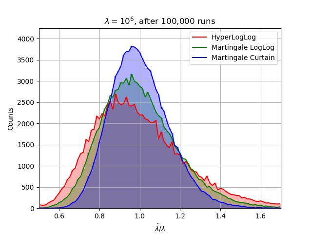
6 Experimental Validation
Throughout the paper we have maintained a possibly unhealthy devotion to asymptotic
analysis, taking m → ∞ whenever it was convenient. In practice m will be a constant, and
possibly a smallish constant. How do the sketches perform in the pre-asymptotic region?
In turns out that the theoretical analysis predicts the performance of Martingale sketches
pretty well, even whem m is small. In the experiment of Figure 3, we fixed the sketch size at
a tiny 128 bits. Therefore HyperLogLog uses m1 = ⌊128/6⌋ = 21 counters. The Martingale
LogLog and Martingale Curtain sketches encode the martingale estimator with a floating point
approximation of λ̂ in 14 bits, with a 6-bit exponent and 8-bit mantissa. Thus, Martingale
LogLog uses m2 = (128 − 14)/6 = 19 counters, and Martingale Curtain uses m3 = 37.14
For larger sketch sizes, the distribution of λ̂/λ is more symmetric, and closer to the
predicted performance. Figure 4 gives the empirical distribution of λ̂/λ over 100,000 runs
when λ = 106 and the sketch size is fixed at 1,200 bits. Here MartingaleCurtain uses m = 400,
and both Martingale LogLog and HyperLogLog use m = 200. The experimental and predicted
relative variances and standard errors are given in Table 2.
Figure 3 The sketch size is fixed at 128 bits. Figure 4 The sketch size is fixed at 1200 bits.
13
The probability of state change Pλ is itself a random variable.
14
It uses the optimal parameterization (q, a, h) = (2.91, 2, 1) of Theorem 4.
ICALP 2021104:18 Non-Mergeable Sketching for Cardinality Estimation
p
Table 2 The relative variance is λ12 Var(λ̂ | λ) and standard error is λ1 Var(λ̂ | λ). The
predictions for Martingale LogLog and Martingale Curtain use Theorems 11, 14, and 17. The
predictions for HyperLogLog are from Flajolet et al. [19, p. 139].
Using 128 bits Using 1200 bits
Sketch Experiment Prediction Experiment Prediction
Var StdErr Var StdErr Var StdErr Var StdErr
HyperLogLog 0.0573 23.94% 0.0549 23.44% 0.00541 7.36% 0.00539 7.35%
Martingale LogLog 0.0348 18.65% 0.0365 19.10% 0.00350 5.91% 0.00347 5.89%
Martingale Curtain 0.0211 14.54% 0.0208 14.43% 0.00189 4.35% 0.00193 4.39%
7 Conclusion
The Martingale transform is attractive due to its simplicity and low variance, but it results in
non-mergeable sketches. We proved that under natural assumptions,15 it generates optimal
estimators automatically, allowing one to design structurally more complicated sketches,
without having to worry about designing or analyzing ad hoc estimators. We proposed the
Curtain sketch, in which each subsketch only needs a constant number of bits of memory, for
arbitrarily large cardinality U .16
The analytic framework of Theorems 7 and 11 simplifies Cohen [14] and Ting [35], and
gives a user-friendly formula for the asymptotic relative variance (ARV) of the Martingale
estimator, as a function of the sketch’s constant κ. We applied this framework to Martingale
Curtain as well as the Martingale version of the classic sketches (MinCount, HLL and PCSA).
Assuming perfect compression, one gets the memory-variance product (MVP) of an
sketch by multiplying its entropy and ARV. It is proved that for linearizable sketches,
Fishmonger is optimal for mergeable sketches [31] (limiting MVP = H0 /I0 ≈ 1.98). In
this paper we proved that in the sequential (non-mergeable) setting, if we restrict our
attention to linearizable sketches, that Martingale Fishmonger is optimal, with limiting
MVP = H0 /2 ≈ 1.63 (Section 5.2). We conjecture that these two lower bounds hold for
general, possibly non-linearizable sketches.
References
1 Noga Alon, Phillip B. Gibbons, Yossi Matias, and Mario Szegedy. Tracking join and self-join
sizes in limited storage. In Proceedings 18th ACM Symposium on Principles of Database
Systems (PODS), pages 10–20, 1999. doi:10.1145/303976.303978.
2 Daniel N Baker and Ben Langmead. Dashing: Fast and accurate genomic distances with
hyperloglog. bioRxiv, 2019. doi:10.1101/501726.
3 Ziv Bar-Yossef, T. S. Jayram, Ravi Kumar, D. Sivakumar, and Luca Trevisan. Counting distinct
elements in a data stream. In Proceedings 6th International Workshop on Randomization and
Approximation Techniques (RANDOM), volume 2483 of Lecture Notes in Computer Science,
pages 1–10, 2002. doi:10.1007/3-540-45726-7_1.
4 Ziv Bar-Yossef, Ravi Kumar, and D. Sivakumar. Reductions in streaming algorithms, with
an application to counting triangles in graphs. In Proceedings 13th Annual ACM-SIAM
Symposium on Discrete Algorithms (SODA), pages 623–632, 2002.
15
insensitivity to duplicates, and unbiasedness
16
Note that an O(log log U )-bit offset register is needed for the whole sketch.S. Pettie, D. Wang, and L. Yin 104:19
5 Ran Ben-Basat, Gil Einziger, Shir Landau Feibish, Jalil Moraney, and Danny Raz. Network-
wide routing-oblivious heavy hitters. In Proceedings of the 2018 Symposium on Architectures
for Networking and Communications Systems (ANCS), pages 66–73, 2018. doi:10.1145/
3230718.3230729.
6 Jarosław Błasiok. Optimal streaming and tracking distinct elements with high probability.
ACM Trans. Algorithms, 16(1):3:1–3:28, 2020. doi:10.1145/3309193.
7 Andrei Z. Broder. On the resemblance and containment of documents. In Proceedings of
Compression and Complexity of SEQUENCES, pages 21–29, 1997. doi:10.1109/SEQUEN.1997.
666900.
8 Thilina Buddhika, Matthew Malensek, Sangmi Lee Pallickara, and Shrideep Pallickara. Synop-
sis: A distributed sketch over voluminous spatiotemporal observational streams. IEEE Trans.
Knowl. Data Eng., 29(11):2552–2566, 2017. doi:10.1109/TKDE.2017.2734661.
9 Philippe Chassaing and Lucas Gerin. Efficient estimation of the cardinality of large data
sets. In Proceedings of the 4th Colloquium on Mathematics and Computer Science Algorithms,
Trees, Combinatorics and Probabilities, 2006.
10 Aiyou Chen, Jin Cao, Larry Shepp, and Tuan Nguyen. Distinct counting with a self-learning
bitmap. Journal of the American Statistical Association, 106(495):879–890, 2011. doi:
10.1198/jasa.2011.ap10217.
11 Min Chen, Shigang Chen, and Zhiping Cai. Counter tree: A scalable counter architecture
for per-flow traffic measurement. IEEE/ACM Trans. Netw., 25(2):1249–1262, 2017. doi:
10.1109/TNET.2016.2621159.
12 Pern Hui Chia, Damien Desfontaines, Irippuge Milinda Perera, Daniel Simmons-Marengo,
Chao Li, Wei-Yen Day, Qiushi Wang, and Miguel Guevara. KHyperLogLog: Estimating
reidentifiability and joinability of large data at scale. In Proceedings of the 2019 IEEE
Symposium on Security and Privacy, pages 350–364, 2019. doi:10.1109/SP.2019.00046.
13 Edith Cohen. Size-estimation framework with applications to transitive closure and reachability.
J. Comput. Syst. Sci., 55(3):441–453, 1997. doi:10.1006/jcss.1997.1534.
14 Edith Cohen. All-distances sketches, revisited: HIP estimators for massive graphs analysis.
IEEE Trans. Knowl. Data Eng., 27(9):2320–2334, 2015. doi:10.1109/TKDE.2015.2411606.
15 Edith Cohen and Haim Kaplan. Tighter estimation using bottom k sketches. Proc. VLDB
Endow., 1(1):213–224, 2008. doi:10.14778/1453856.1453884.
16 Marianne Durand and Philippe Flajolet. Loglog counting of large cardinalities. In Proceedings
11th Annual European Symposium on Algorithms (ESA), volume 2832 of Lecture Notes in
Computer Science, pages 605–617. Springer, 2003. doi:10.1007/978-3-540-39658-1_55.
17 R. A. Leo Elworth, Qi Wang, Pavan K. Kota, C. J. Barberan, Benjamin Coleman, Advait
Balaji, Gaurav Gupta, Richard G. Baraniuk, Anshumali Shrivastava, and Todd J. Treangen.
To petabytes and beyond: recent advances in probabilistic and signal processing algorithms
and their application to metagenomics. Nucleic Acids Research, 48(10):5217–5234, 2020.
doi:10.1093/nar/gkaa265.
18 Cristian Estan, George Varghese, and Michael E. Fisk. Bitmap algorithms for counting
active flows on high-speed links. IEEE/ACM Trans. Netw., 14(5):925–937, 2006. doi:
10.1145/1217709.
19 Philippe Flajolet, Éric Fusy, Olivier Gandouet, and Frédéric Meunier. HyperLogLog: the
analysis of a near-optimal cardinality estimation algorithm. In Proceedings of the 18th
International Meeting on Probabilistic, Combinatorial, and Asymptotic Methods for the Analysis
of Algorithms (AofA), 2007.
20 Philippe Flajolet and G. Nigel Martin. Probabilistic counting algorithms for data base applic-
ations. J. Comput. Syst. Sci., 31(2):182–209, 1985. doi:10.1016/0022-0000(85)90041-8.
21 Michael J. Freitag and Thomas Neumann. Every row counts: Combining sketches and sampling
for accurate group-by result estimates. In Proceedings of the 9th Biennial Conference on
Innovative Data Systems Research (CIDR), 2019.
ICALP 2021You can also read


