Sea level changes at Tenerife Island (NE Tropical Atlantic) since 1927
←
→
Page content transcription
If your browser does not render page correctly, please read the page content below
JOURNAL OF GEOPHYSICAL RESEARCH: OCEANS, VOL. 118, 4899–4910, doi:10.1002/jgrc.20377, 2013

Sea level changes at Tenerife Island (NE Tropical Atlantic) since 1927
Marta Marcos,1 Bernat Puyol,2 Francisco M. Calafat,3,4 and Guy Woppelmann5
Received 29 May 2013; revised 27 August 2013; accepted 27 August 2013; published 2 October 2013.

[1] Hourly sea level observations measured by five tide gauges at Santa Cruz harbor
(Tenerife Island), in the Northeastern Tropical Atlantic, have been merged to build a
consistent and almost continuous sea level record starting in 1927. Datum continuity was
ensured using high precision leveling information. The time series underwent a detailed
quality control in order to remove outliers, time drifts, and datum shifts. The resulting sea
level record was then used to describe the low frequency (interannual to decadal) sea level
variability at Tenerife. It was found that at interannual and longer time scales, the observed
sea level changes are primarily driven by steric sea level variations. Such steric changes are
originated by coastal trapped waves induced by longshore winds along the continental coast
and propagate poleward. Observed sea level rise at Tenerife was 2.09 6 0.04 mm/yr since
1927. According to the hydrographic observations in the area, only half of this trend was
attributed to steric sea level changes for the top 500 m, at least since 1950.
Citation: Marcos, M., B. Puyol, F. M. Calafat, and G. Woppelmann (2013), Sea level changes at Tenerife Island (NE Tropical
Atlantic) since 1927, J. Geophys. Res. Oceans, 118, 4899–4910, doi:10.1002/jgrc.20377.

1.    Introduction                                                            tide gauge observations at Brest dating back to the 18th
                                                                              century from old archives. Other notable exercises of data
   [2] Long-term mean sea level changes at time scales of                     archaeology can be found in Testut et al. [2010], who have
years to decades and centuries display a large spatial vari-                  provided sea level observations at Saint Paul Island (Indian
ability as a result of the regional distribution of its forcing               Ocean) from late 19th century, and Woodworth et al.
mechanisms. The description and understanding of this var-                    [2010] that linked old sea level measurements from the
iability is constrained by the uneven geographical coverage                   19th century with present day observations at Falkland
of sea level observations and by the limited number of con-                   Islands (South Atlantic). Likewise, Watson et al. [2010]
sistent long time series. Only during the last two decades,                   recovered sparse sea level observations of the 20th century
satellite observations have provided high quality nearly                      in Macquarie Island (SW Pacific) whereas Marcos et al.
global sea level measurements that have proven extremely                      [2011] built a continuous sea level time series at Cadiz
powerful. Longer term observations however, are much                          (Southern Spain) after recovering historical tide gauge
scarcer ; according to the PSMSL data base [Holgate et al.,                   observations from 1882 to 1924 and linking them with a
2013; www.psmsl.org], only around 120 sea level tide                          modern nearby record. More recently, Talke and Jay
gauge records worldwide are longer than 80 years and its                      [2013] described historical sea level measurements in the
geographical distribution is mostly concentrated on the                       Pacific and the coasts of North America, starting during the
northern hemisphere and along continental shores, which                       mid-19th century, and identified 600 station years of tabu-
may significantly bias the estimation of global and regional                   lated data, and Dangendorf et al. [2013] used digitized
sea level trends and accelerations.                                           mean sea level observations at Cuxhaven for the period
   [3] In an attempt to overcome the limitations of the                       1871–2008 to study the climatic and meteorological contri-
sparse sea level data set, many efforts are presently devoted                 butions to sea level related to large scale atmospheric
to the extension of the current historical sea level data base.               forcing.
Wöppelmann et al. (2006, 2008) recovered and analyzed                            [4] In 2011, the Global Sea Level Observing System
                                                                              (GLOSS) Group of Experts recognized the potential of tide
Additional supporting information may be found in the online version of
                                                                              gauge data rescue and developed a questionnaire aimed at
this article.
                                                                              identifying details of archived observations. The responses,
   1
    IMEDEA, UIB-CSIC, Esporles, Spain.                                        compiled and analyzed by Caldwell [2012], revealed that
   2
    Instituto Geografico Nacional, Madrid, Spain.                             there still exists a huge amount of historical tide gauge
   3
    College of Marine Science, University of South Florida, St. Petersburg,   measurements in nonelectronic format. A significant part of
Florida, USA.                                                                 such data correspond to long time series that could be used
   4
    National Oceanography Centre, Southampton, UK.
   5
    LIENSS, Universite de la Rochelle-CNRS, La Rochelle, France.             in the assessment of long-term sea level rise and changes in
                                                                              extreme high water events [Caldwell, 2012]. The present
  Corresponding author: M. Marcos, IMEDEA (UIB-CSIC), Miquel
Marquès, 21, ES-07190 Esporles, Spain (marta.marcos@uib.es)
                                                                              work represents an example of how the recovery of histori-
                                                                              cal tide gauge data can provide useful information for
©2013. American Geophysical Union. All Rights Reserved.                       present-day research on climate in an area poorly sampled
2169-9275/13/10.1002/jgrc.20377                                               such as the Tropical Northeast Atlantic Ocean. The

                                                                          4899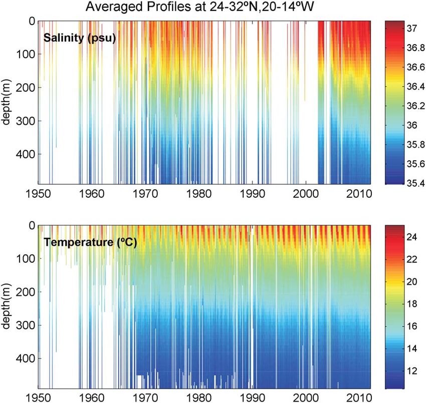
MARCOS ET AL.: SEA LEVEL AT TENERIFE ISLAND

objective of this work is twofold: first, it is aimed at            [5] Tenerife Island is part of the Canary Archipelago,
constructing a long and consistent hourly sea level record       located at latitudes 28 –29 N and about 300 km offshore
from the information obtained from log books, nondigitized       the African coast (Figure 1). The archipelago is located on
observations, leveling surveys and modern sea level              the path of the Canary Current, a branch of the Azores Cur-
records at Tenerife Island. Second, it intends to use this       rent flowing equatorward along the West African coast up
new sea level time series to describe the sea level variabili-   to latitudes 20 –25 N and driven by the prevailing south-
ty at Tenerife Island and to get insight into the underlying     erly Trade winds [Navarro-Perez and Barton, 2001;
processes that drive such variability.                           Hernandez-Guerra et al., 2001]. Strong coastal upwelling

         Figure 1. (top) Map and location of the Santa Cruz harbor. (bottom) Santa Cruz harbor and sites of the
         tide gauges: label 1 corresponds to TN011 (southern pier) and label 2 corresponds to TN012 and TN013
         (northern pier).

                                                             4900
MARCOS ET AL.: SEA LEVEL AT TENERIFE ISLAND

occurs off North West Africa, seasonally and interannually         (location 2 in Figure 1), with a new stilling well of 7 m
modulated by the wind variability. The bathymetry around           deep and of 1 m diameter. As in the first case, water was fil-
Tenerife is steep with a narrow shelf. This makes this loca-       tered through the pier to reach the well and no direct con-
tion particularly suitable for the study of the sea level          nection was built with the open sea. This time the reference
changes as it is expected to reflect sea level variability in       benchmark was part of the national leveling network
the deep nearby ocean. Furthermore, its location in a poorly       (NAPG991, see Table 1 and Figure 2). The two tide gauges
sampled region makes its study even more valuable.                 were then moved to the new location. However, since the
                                                                   beginning, many problems were reported with the Thomson
                                                                   tide gauge, likely attributed to the substitution of the perfo-
2. Tide Gauge Records at Santa Cruz (Tenerife                      rated tape connecting the pulley with the floating device,
Island)                                                            originally metallic, by one made of nylon. Log books docu-
                                                                   ment continuous drifts of the measurements which obliged
2.1. A Brief Historical Overview                                   to recalibrate the instrument every few days. In 1965, the
   [6] In 1923, the Spanish Geographical Institute (IGN)           perforated tape, the floating device and the pulley were all
projected the installation of a tide gauge station at Tenerife     replaced, and the instrument operated properly since then.
Island with the aim of accurately determining the mean sea         The scale factor was changed to 1/10. The Mier instrument
level at the Canary Islands archipelago. The Spanish engi-         continued operating until 1975. In 1990, the port authority
neer Manuel Cifuentes took on the responsibility of defin-          changed the location of the tide gauge station to a new well,
ing the best location for the instrument, which was finally         very close to the former (location 2 in Figure 1), on the
established on the southern pier of Santa Cruz harbor (loca-       northern pier. The Thomson tide gauge was substituted by
tion 1 in Figure 1), under construction by that time. The          an AOTT tide gauge, with a vertical scale factor of 1/5 and
stilling well was 3.4 m deep and had a diameter of 1.2 m. It       was referenced to the leveling benchmark NAPH413 (Table
was not directly connected to the sea; instead, sea water          1 and Figure 2). Sea level observations of the new tide
was filtered in and out through the porous pier due to pres-        gauge started in 1991; however, very soon it was found out
sure differences caused by changing water levels. High fre-        that the new well often suffered from obstruction problems.
quency sea level variations, mostly due to wind waves,             These were solved in 1993 and the reference benchmark
were thus filtered out. However, filtering also affected long        was subsequently changed to the new NGU320 (Table 1
waves, such as tides, by delaying their timing (without any        and Figure 2). The tide gauge has since then been working.
effect on their amplitude though). The leveling reference of       A digital encoder was installed in 1997, providing sea level
the tide gauge measurements was defined as a benchmark              measurements with a time interval of 10 min in a digital for-
fixed at the well pithead. Two instruments were installed           mat. In 2007, a new radar Vega tide gauge was installed on
simultaneously on the same well, both recording sea level          the same pier with a sampling interval of 5 min (1 min since
changes on a continuous tidal chart. The principal was a           November 2008). In parallel, the Spanish Port Authority in-
Thomson mechanical floating tide gauge, with a vertical             stalled an acoustic SONAR tide gauge in 1992 nearby the
scale factor of 15/100, and the secondary was a Mier syphon        location of the TN013 floating tide gauge (PdE in Figure 1).
type tide gauge, whose vertical scale factor was 1/20, thus        This was part of the national tide gauge network operated
less accurate. The purpose of this secondary tide gauge was        and maintained by the Spanish Port Authority (PdE,
to serve as an additional quality control of the main instru-      www.puertos.es). It provided 5 min sea level observations
ment and, in case of malfunctioning of the Thomson, it             with respect to the benchmark SS412 (Table 1 and Figure 2).
could also be used to correct/substitute the potential wrong       In 2009, the same agency substituted the acoustic tide gauge
observations. Observations started on 3 January 1927 and           by a radar MIROS tide gauge, which is still in operation.
both tide gauges were operating until 1936, when measure-
ments were suddenly interrupted due to the Spanish Civil           2.2. Sea Level Observations
War. In 1940, the observations started over again. Many              [7] Sea level observations were obtained from five tide
problems related to the malfunctioning of the Thomson tide         gauge records located at Santa Cruz harbor (Tenerife Island)
gauge were reported later on from 1954 until 1956, when            that operated at distances less than 500 m from each other.
measurements were definitely stopped. In 1958, a new loca-          The characteristics and periods of operation of the instru-
tion was delivered by the port authority on the northern pier      ments, outlined in the previous section, are summarized in

Table 1. Characteristics of the Tide Gauge Records
Tide Gauge Record      Agency       Manufacturer            Period of Operation           Sampling           Benchmark

TN011                   IGN         Thomson                       1927–1956           Hourly                 Inner BM
TN012                   IGN         Thomson                       1958–1990           Hourly                 NAPG991
TN013                   IGN         AOTT                         1992–ongoing         Hourly (1993)
Secondary               IGN         Mier                          1927–1975           Hourly                 Same as primary tide
                                                                                                               gauge for each period
Secondary               IGN         Vega                         2007–ongoing         5 min (5/2009)

                                                             4901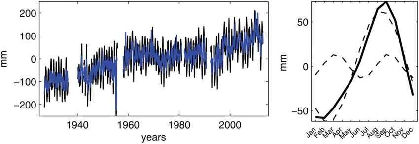
MARCOS ET AL.: SEA LEVEL AT TENERIFE ISLAND

                                                                 and presented a clear seesaw shape. This was certainly
                                                                 related to the malfunctioning problems detected after the
                                                                 change to TN012 location and reported in the historical
                                                                 documentation. For the entire period of TN011 and TN012,
                                                                 1927–1990, raw observations were calibrated on the basis
                                                                 of hourly interpolated ‘‘tide gauge constants.’’
                                                                    [9] The secondary Mier tide gauge observations, for
                                                                 which the ‘‘tide gauge constants’’ were provided on a daily
                                                                 basis, were also calibrated as described above for the pri-
                                                                 mary TN011 and TN012 records.
                                                                    [10] For TN013 record, only values for 1993 unevenly
                                                                 distributed (8–10 values per month) were provided. The
                                                                 averaged ‘‘tide gauge constant’’ was computed for the
                                                                 available period, after discarding outliers greater or lower
                                                                 than the standard deviation of the total series of constants.
                                                                 The obtained mean parameter was used to calibrate all
Figure 2. Relative heights (in m) between benchmarks.            observations for the period 1992–1997.
See Table 1 for the correspondence to tide gauges. Years of         [11] Calibrated sea level observations of TN011, TN012,
each leveling survey are indicated in parenthesis.               and TN013 were referred to four different benchmarks (Ta-
                                                                 ble 1). High precision leveling information was used to link
Table 1 (data from the secondary Vega tide gauge was not         the benchmarks with the aim of building a single sea level
used in this study). TN011, TN012, and TN013 refer herein-       time series with datum continuity. A total of 10 leveling
after to the observations of the primary tide gauge. Hourly      surveys were carried out in the vicinity of the tide gauges
sea level data of TN011 and TN012 (i.e., from 1927 to            between 1921 and 2010. The resulting heights were care-
1990) corresponded to hand-written observations obtained         fully checked to detect eventual shifts between two subse-
from the tidal charts and stored in log books that have been     quent surveys and to identify the most stable benchmarks.
archived at the Spanish National Geographic Institute (IGN)      For all cases examined, the closure errors of the leveling
in Madrid. All these observations were digitized and con-        surveys were smaller than 2 mm at each path, ensuring thus
verted into electronic format. The same applies to observa-      the reliability of the results. It was found that all bench-
tions of TN013 until 1997. After then, sea level observations    marks used to link the tide gauge references were stable,
were acquired as a digital output with a temporal sampling       except for the inner benchmark used at TN011 record. In
of 10 min. The PdE tide gauge has provided sea level meas-       this case, two surveys performed in 1921 and 1960 detected
urements every 5 min since 1992 in a digital format. This        a shift with respect to the benchmark NAP380 of 11 mm,
time series has been used as an additional quality control of    or equivalently 0.27 mm/yr of subsidence if we assume that
the TN013 time series and to fill in data gaps when needed.       the change is linear. This correction was therefore applied
Additionally, a few years of digitized data of the secondary     in the form of a linear trend to the TN011 record. The rela-
Mier tide gauge (1955–1957 and 1958–1965) were also              tive heights between benchmarks are schematically shown
available and were used to quality control. Five different       in Figure 2. All sea level observations from the three
benchmarks were used since 1927, as indicated in Table 1.        records TN011, TN012, and TN013 were referred to the
The relationships among benchmarks are discussed below.          common datum NGR333, which was considered as the
                                                                 most adequate due to its stability and location close to
2.3. Data Calibration and Datum Continuity                       the modern tide gauge. This benchmark is part of the high
   [8] Until 1997, sea level observations of the floating         precision Spanish national leveling network. The result was
gauges (records TN011, TN012, and TN013) were pro-               a consistent hourly sea level record for the period 1927–
vided as noncalibrated data. The information needed to           2012; this is the sea level time series that will be used here-
convert these noncalibrated tidal chart readings into actual     inafter for the subsequent analysis. In addition, the Mier
sea level values with respect to a given benchmark is            secondary and the PdE time series were also referred to the
referred to as the ‘‘tide gauge constant.’’ This parameter       same benchmark, in order to be used as complementary
measures the difference between noncalibrated values and         data to the main longest record.
the actual distance of sea level to the benchmark and, in ab-
sence of technical problems, it should remain unchanged,         2.4. Quality Control and Tidal Analysis
as its name suggests. Variations of this parameter indicate         [12] Hourly values larger or lower than three times the
vertical movements with respect to the tide gauge bench-         standard deviation of the total time series were considered
mark which can be attributed to changes in the tide gauge        as outliers and were consequently removed. Smaller but
reference, for instance if all or part of the tide gauge has     persistent outliers were also observed during the period
changed position for maintenance, but also to recalibration      1958–1964, which were consequence of the recalibration
of the instrument due to malfunctioning. The ‘‘tide gauge        procedures as described above. Little can be done to
constants’’ were provided daily or half-daily for TN011          improve these data, except to substitute them with the sec-
and TN012 records (1927–1990). A simple visual examina-          ondary tide gauge observations. We decided to substitute
tion of the ‘‘tide gauge constants’’ time series revealed that   the primary Thomson sea level observations with those from
the series was not always stable. In particular, for the         the less accurate but well calibrated Mier tide gauge for the
period 1958–1964, the series was far from homogeneous            period January 1958 to December 1964. In 1955–1956, a

                                                             4902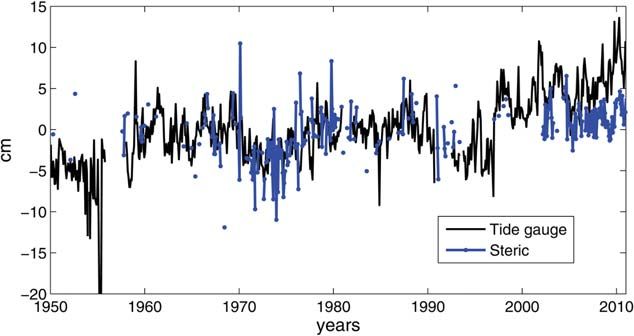
MARCOS ET AL.: SEA LEVEL AT TENERIFE ISLAND

                                                                       [14] All the tidal constituents estimated using the refer-
                                                                    ence period were used to build an hourly tidal time series
                                                                    for the entire length of the record (1927–2012). The objec-
                                                                    tive was to identify periods with time drifts or shifts, poten-
                                                                    tial changes in the reference time and malfunctioning of the
                                                                    instrument. To do so, a detailed comparison between tidal
                                                                    predictions and observations was done by computing lag
                                                                    correlations between the two time series on a monthly ba-
                                                                    sis. Since the time lags between both series were expected
                                                                    to be smaller than the sampling period (1h), the time series
                                                                    were first linearly interpolated to 1 min time interval. Lag
Figure 3. Hourly sea level time series referred to the              correlations were then computed for each calendar month
NGR333 benchmark.                                                   and the time lag of maximum correlation was identified.
                                                                    The resulting time lags of maximum correlation are repre-
datum shift was also observed (not shown) which was not             sented in Figure 4. The largest time lags, with values up to
documented in the log books. In this case, the Mier data pre-       100 min, were found for the years 1992–1994, during
sented a similar problem than the primary record and could          which sea level oscillations appeared anomalously smaller
not be used to correct it. Therefore, in absence of any other       than average (see Figure 3). This result suggested malfunc-
information, the period November 1955 to December 1956              tioning of the instrument due to an obstruction of the stil-
was removed. The resulting hourly sea level time series, af-        ling well which induces variations of the tidal amplitudes
ter these first corrections were applied and referred to the         and phases [e.g., Agnew, 1986; Pugh, 1987]. It is thus in
NGR333 benchmark, is plotted in Figure 3. In the follow-            agreement with the reported problems in the log books.
ing, a more detailed and careful quality control based on           These years were consequently removed from the record.
tidal analysis is performed.                                        Instead, hourly sea level observations of the PdE tide gauge
   [13] A tidal analysis was applied for the period 1965–           (that were referred to the same common benchmark) were
1977. This time interval was identified as the continuous            used to fill in these data gaps. Additionally, for the entire
most stable longest period and was therefore used to esti-          common period, starting in July 1992, both time series
mate the most reliable tidal constituents for the study site.       were compared and PdE was used to fill in data gaps of the
The tidal analysis was performed using the t_tide software          original series whenever possible.
package [Pawlowicz et al., 2002] and only those tidal con-             [15] During the period 1958–1964, it was found a time
stituents, among the initial 143, with a signal-to-noise ratio      lag of 1 h, suggesting a shift of the internal clock starting in
larger than 2 were considered. The estimated tidal ampli-           1965. Unfortunately, no historical documentation could be
tudes of the major constituents (i.e., those with amplitudes        found confirming this hypothesis. This period was cor-
larger than 1 cm) are listed in Table 2, together with their        rected simply by advancing the timing 1 h. Finally, the re-
corresponding confidence intervals. Annual and semiannual            cord corresponding to TN011 (1927–1956) appeared to be
cycles were removed as their origin is mostly nonastronom-          in advance by an average of 36 min with respect to the cur-
ical. The estimated tidal phases have not been listed               rent timing. The likely explanation for this discrepancy is
because they depend on the delay induced by the water fil-           that the delay induced by water filtering through the pier
tering inside the well and are thus not representative of the       was different at the well locations of TN011 and TN012.
actual tidal phases at Tenerife. Results indicated that Ten-        This effect does not affect the quality of the observations
erife has a semidiurnal tidal regime, with tidal oscillations       and was thus not corrected.
between 61.5 m and with M2 being the largest constituent
(72 cm).                                                            3.   Other Data Sets and Methodology
                                                                       [16] In order to investigate the observed sea level varia-
                                                                    tions at Tenerife and its forcing mechanisms, the data sets
Table 2. Major Tidal Constituents (With Amplitudes Larger           listed below were used as complementary data.
Than 1 cm) at Tenerife
Tidal Constituent      Frequency (hours)        Amplitude (cm)

Q1                           26.87                1.37 6 0.04
O1                           25.82                4.40 6 0.04
P1                           24.07                2.09 6 0.05
K1                           23.93                5.89 6 0.05
2N2                          12.91                2.10 6 0.05
MU2                          12.87                2.94 6 0.05
N2                           12.66                15.06 6 0.05
NU2                          12.63                2.83 6 0.05
M2                           12.42                72.57 6 0.05
L2                           12.19                2.25 6 0.07
T2                           12.02                1.63 6 0.05
                                                                    Figure 4. Lags of maximum correlation between obser-
S2                           12.00                27.40 6 0.05
K2                           11.97                6.76 6 0.04
                                                                    vations and tidal predictions computed for each calendar
                                                                    month.

                                                                 4903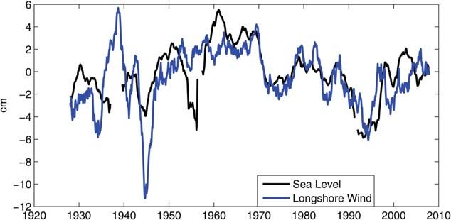
MARCOS ET AL.: SEA LEVEL AT TENERIFE ISLAND

   [17] Monthly gridded mean sea level pressure and wind         pressure for periods shorter than 20 days and the inverted
stress fields were obtained from the 20th century Reanaly-        barometer (IB) correction for longer periods.
sis data set [Compo et al., 2011], with a grid spacing of           [20] In addition to altimetric observations, other tide
2  2 and spanning the period 1871–2010. These data            gauge records were also considered. Monthly mean sea level
sets were used to quantify the local response of sea level to    tide gauge time series at Cascais, Santander, Brest, and New-
atmospheric pressure and wind. Atmospheric pressure              lyn were downloaded from the Permanent Service for Mean
fields were used to quantify the inverted barometer (IB)          Sea Level (PSMSL) data repository (www.psmsl.org). All
contribution to sea level as:                                    records considered are Revised Local Reference (RLR), that
                                                                 is, they have been checked and corrected for local datum
                                1                              continuity over time relative to benchmarks in the vicinity
                        IB ¼        P a  Pa :             ð1Þ
                               g0                               [Holgate et al., 2013].
                                                                    [21] The contribution of density changes to sea level at
where Pa is the atmospheric pressure, g the gravity acceler-     Tenerife was investigated using hydrographic observations.
ation, the bar denotes averaging over the global oceans,         Ocean temperature (T) and salinity (S) profile data were
and 0 is the reference water density.                           obtained from the EN3 dataset in its version v2a [Ingleby
   [18] Besides the barotropic response of local atmospheric     and Huddleston, 2007] available at the Met Office Hadley
pressure and winds, Calafat et al. [2012] proved that            Centre (http://www.metoffice.gov.uk/hadobs/en3/) for the
coastal sea level variations on the eastern boundary of the      period 1950–2011 and located within the area 24–32 N and
North Atlantic northward of about 25 N display a baro-          20–14 W. The profiles version with time varying XBT cor-
clinic response to longshore winds. In essence, when the         rections [Wijffels et al., 2008] was selected. T and S pro-
wind blows parallel to the coast with the coast on its left it   files that did not pass the quality controls were discarded
displaces surface water offshore through Ekman transport.        for the analysis. For each calendar month of the entire pe-
Because there can be no flow normal to the coast, the dis-        riod 1950–2011, the corresponding T and S profiles were
placed surface water needs to be replaced by denser water        first interpolated onto the same depths from 10 to 500 m at
from deeper levels, which pushes the thermocline upward          10m depth intervals and were afterward averaged out in
and thus results in a decrease in the steric sea level. This     order to build a single monthly profile, whenever possible.
effect, however, is not purely local because the induced         Standard deviations for each depth were also computed.
changes in the thermocline can propagate poleward along             [22] Additionally, hydrographic observations from the
the coast in the form of boundary waves affecting a large        RAPROCAN program (http://www.oceanografia.es/rapro-
portion of the coast northward of the region of forcing          can/) were kindly provided by the Spanish Institute of
[Gill, 1982]. Following Calafat et al. [2012], the response      Oceanography. The data belong to a monitoring program of
to the longshore wind was quantified using the expression:        the deep ocean around the Canary Islands and consists of a
                                                                 hydrographic section at 29.5 N and between 13 and 24 W
                   Zy                                          carried out twice a year. Data are available for only a few
                                     y  y0
                         s y0 ; t          dy0 :         ð2Þ   surveys in 1997, 1998, and from 2004 onward. T and S pro-
                                       c
                   y0                                            files are measured at 30 hydrographic stations down to the
                                                                 bottom and at 1 m depth intervals. This data set has been
where c is the internal wave velocity (1–3 m/s),  s is the      carefully edited, calibrated, and quality controlled. RAP-
wind stress parallel to the coast, y0 is the zero latitude and   ROCAN data lying within the target area were processed in
y ¼ 28 N corresponds to the latitude of Tenerife. For the       the same way as described above for EN3 profiles and were
integration, we used the International Comprehensive             integrated in the analysis.
Ocean-Atmosphere Data Set (ICOADS) (http://www.esrl.-               [23] T and S profiles were used to compute the steric sea
noaa.gov/psd/) wind data as they provide actual ground           level by integrating down to a predefined reference pres-
measurements of wind with a relatively good coverage of          sure (Pref) the specific volume anomalies ():
the African continental shelf at the latitudes of interest.
This data set consists of monthly mean wind observations                                        Z0
on a global 2  2 grid spanning the period 1800 to pres-                                  1
                                                                                   Steric ¼            ðT ; S Þ dp:       ð3Þ
ent. In order to obtain a continuous time series of the inte-                               g
                                                                                                Pref
grated longshore wind, wind data during months in which
wind observations are not available are obtained from the
20th century reanalysis [Compo et al., 2011].
   [19] Other sea level data sets were also included in the      4. Long-Term (Monthly to Decadal) Sea Level
analysis in order to investigate the regional sea level coher-
ency. Monthly gridded mean sea level anomalies with a            Variability at Tenerife
map spacing of 1/4  1/4 were downloaded from AVISO              [24] Quality controlled hourly observations were used to
data server (www.aviso.oceanobs.com). These data consists        compute monthly mean sea level. Only those months with
of a multisatellite global product, which combines up to         at least 50% of valid observations were considered. The
four altimetric satellites and spans the period from October     resulting monthly time series is plotted in Figure 5 (left
1992 to present. All geophysical corrections were applied,       plot, black line). The monthly time series is available as
including the so-called dynamic atmospheric correction           supporting information. The most prominent signal in the
(DAC) [Volkov et al., 2007]. DAC consists of a combina-          monthly time series is the seasonal cycle. The mean ampli-
tion of a barotropic model forced by winds and atmospheric       tudes and phases of the annual and semiannual signals were

                                                             4904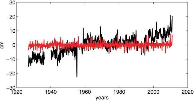
MARCOS ET AL.: SEA LEVEL AT TENERIFE ISLAND

         Figure 5. (left) Monthly mean sea level with (black) and without (blue) seasonal cycle. (right) Mean
         annual and semiannual cycles (dashed lines) and mean seasonal cycle (solid line).

estimated using least square fitting of two sinusoidal sig-        routinely calculated using vertically integrated ocean mod-
nals. It was found that the seasonal cycle accounts for 34%       els. However, only rarely this barotropic component is
of the total monthly sea level variance. The mean annual          available for a long-term period. Unfortunately, there is
and semiannual amplitudes obtained were 6.3 cm and 1.3            not, to our knowledge, such kind of information for the
cm, the first peaking in August and the second in February         area of the Canary Islands for the last decades; therefore,
(Figure 5, right plot). The monthly deseasoned sea level re-      the barotropic component of sea level at Tenerife was
cord is plotted in Figure 5 (blue line). Despite having           quantified using an empirical relationship between mean
removed the mean seasonal cycle, there is still residual          sea level and atmospheric pressure and wind stress fields.
energy evident at the annual frequency. The reason is that the    The closest grid points of mean sea level pressure and wind
seasonal cycle varies both in space and time [Marcos and          stress from the 20th Century Reanalysis data to the tide
Tsimplis, 2007; Barbosa et al., 2008). Therefore, its temporal    gauge were chosen as representative of the forcing fields at
variability was explored by estimating the annual and the         its location. To ensure global ocean mass conservation, the
semiannual signals for 5 year periods, overlapping year-to-       averaged sea level pressure over the global oceans (which
year. The resulting changes in the annual and semiannual          is time-varying in general) was subtracted from the local
amplitudes, together with their standard errors, are plotted in   sea level pressure time series at Tenerife. We must remark
Figure 6 (top). The standard deviations are 1 cm and 0.5 cm       that the steep orography of Tenerife Island partly deter-
for the annual and semiannual amplitudes, respectively. An-       mines the local winds of the island. Hence, the atmospheric
nual amplitudes change up to 3 cm within the observation pe-      re-analysis has a too coarse spatial resolution to capture
riod, with smaller values between 1960s and 1980s. A look at      such local features. Therefore, the barotropic contribution
the seasonal winter and summer averages (Figure 6, bottom)        determined with an empirical relationship will likely miss
indicates that the decrease in the annual cycle amplitudes        this local variability.
was due to higher than average winter sea levels, while              [26] A multiple regression was applied using atmos-
summer sea levels displayed smaller interannual variability.      pheric pressure and zonal and meridional wind stress time
                                                                  series as predictors for the common period:
4.1. The Contribution of Local Atmospheric Pressure
and Wind                                                                 Sea Level ¼ aP þ bWindStressX þ cWindStressY
  [25] The barotropic response of sea level to the com-
bined effect of atmospheric pressure and wind is nowadays           [27] All time series were detrended and deseasoned prior
                                                                  to the analysis. The regression coefficients a, b, and c were
                                                                  obtained using least squares. Our intention was to keep the
                                                                  long-term contributions of atmospheric pressure and wind
                                                                  to the barotropic term; to do so, we have used deseasoned,
                                                                  but not detrended, forcing fields when the barotropic com-
                                                                  ponent was estimated based on the coefficients a, b, and c.
                                                                    [28] The regression coefficients for Tenerife sea level re-
                                                                  cord resulted in a¼ 0.58 cm/mbar, b¼ 43.77 cm/(N/m2)
                                                                  and c¼ 20.18 cm/(N/m2). The overall variance reduction
                                                                  in monthly sea level accounted for by the barotropic contri-
                                                                  bution was 9%, according to this regression model. If only
                                                                  atmospheric pressure is considered the variance reduction
                                                                  decreases to 5%. The monthly mean sea level time series
                                                                  (deseasoned) and the predicted barotropic contribution at
                                                                  Tenerife are plotted in Figure 7. The most significant differ-
Figure 6. (top) Temporal variability of the annual and            ence between the two time series is the sea level rise
semiannual amplitudes of the seasonal cycle, computed for         observed in total sea level, which is attributed to causes
5 years period overlapping year-to-year. (bottom) Seasonal        other than the direct atmospheric forcing. The linear sea
winter (DJF) and summer (JJA) sea level averages.                 level trend estimated from monthly deseasoned observations

                                                              4905
MARCOS ET AL.: SEA LEVEL AT TENERIFE ISLAND
Figure 8. Detrended and smoothed with a 2 year running
Figure 7. Monthly mean sea level (black) and the baro- mean sea level at Tenerife (black) and integrated longshore
tropic contribution obtained from the multiple regression wind at 28 N.
model (red). Both time series are deseasoned.
of the exceptionally large longshore wind variations around
was 2.0760.05 mm/yr (uncertainties quoted correspond 1940. Such longshore wind changes are not realistic and
hereinafter to standard errors) for the entire period 1927– are due to the uneven distribution of wind observations
2010, whereas when the barotropic contribution was over the ocean and the lack of data, especially during the
removed it became 2.04 6 0.04 mm/yr. This is consistent World War II. When only the period from 1958 onward
with the barotropic component having an overall trend of was considered, the correlation increased to 0.8. Lag corre-
0.04 6 0.02 mm/yr. Seasonal differences in the long-term lations indicated that the longshore wind contribution
barotropic contribution were found to be slightly higher dur- appeared to be 1 month in advance with respect to the sea
ing autumn and winter (0.06 mm/yr) than during spring and level at Tenerife. This is in agreement with Calafat et al.
summer (0.01 and 0.03 mm/yr, respectively). [2012] and Sturges and Douglas [2011], despite their
records were all along continental shores.
4.2. Interannual and Decadal Sea Level Variations [30] Changes in steric sea level associated with long-
[29] After removing the barotropic sea level component, shore wind forcing of the thermocline are dominant at dec-
the residual mean sea level changes display large decadal adal scales, but nothing can be said about its longer term
sea level variability, as suggested by Figure 7. The mecha- contribution due to the limitations of the wind observations.
nisms driving decadal sea level variability along the west- For this reason, the steric contribution (equation (3)) to
ern European coasts were recently explored by Calafat et long-term sea level trend has been explored using hydro-
al. [2012]. They found that, at decadal time scales, sea graphic data. The resulting monthly averaged T and S pro-
level fluctuations are highly correlated along the western file time series are plotted in Figure 9. Hydrographic
European coast and provided evidence that the observed observations around Tenerife revealed a deepening of the
sea level variability was linked to the poleward propagation thermocline during the last four decades and heating of the
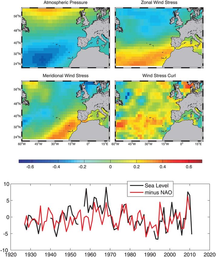
of wind-driven steric sea level fluctuations along the coast. upper waters (down to 100 m). Likewise, although very
Thus, other mechanisms influencing decadal sea level vari- scarce, S observations suggested significant S increases
ability, such as local surface heat fluxes, and mass redistrib- during the years 2000s with respect to the 1970s (this is
ution in the north Atlantic linked to changes in the strength reflected in the deepening of the isohalines). It is worth
of the subtropical gyre, were discarded. They proved so for mentioning that the same effect of rising mean T and salini-
tide gauges at latitudes higher than 40 N, whereas Sturges fication of the upper waters can also be detected in the
and Douglas [2011] demonstrated the same relationship at RAPROCAN observations. We thus consider that this
Cascais (39 N). Calafat et al. [2012] suggested, on the ba- result is robust.
sis of the output of a numerical model, that the correlation [31] Steric sea level was computed for each monthly
between longshore wind effects and sea level at decadal averaged profile of T and S fully covering the top 500 m
scales may also hold at latitudes as low as 28 N. We there- following equation (2). Though this is a restrictive crite-
fore compared decadal sea level at Tenerife with longshore rion, it is the only way to ensure consistency among all
winds. Following Calafat et al. [2012], the effect of wave- steric values. The reference level of 500 m was chosen as a
propagation is accounted for by integrating the longshore compromise between the number of profiles available and
wind from the equator up to the latitude of Tenerife their representativeness of the steric changes. After desea-
(28 N; equation (2)). The resulting time series of the soning, the resulting steric sea level was compared with
integrated longshore wind, detrended and smoothed with a observed sea level at the tide gauge with the barotropic cor-
2 years running mean, are compared with the sea level (cor- rection applied (Figure 10). The correlation between the
rected for local atmospheric and wind effects) from the tide two time series, although statistically significant, was low
gauge record at Tenerife in Figure 8. Note that the inte- (0.22) at interannual time scales. However, the correspon-
grated longshore wind as calculated here provides an esti- dence at longer periods was much better. When a 12
mate of the variability of the sea level response to the months running average was applied to both time series
longshore wind but not the right magnitude [Calafat et al., (not shown), the correlation became 0.43, despite the num-
2012]; thus it was rescaled for comparison with observed ber of observations was significantly reduced due to the
sea level. The correlation between these two series was 0.6 discontinuities in the steric record. Likewise, steric sea
(significant at the 95% confidence level), and this in spite level was correlated with the longshore wind contribution
4906MARCOS ET AL.: SEA LEVEL AT TENERIFE ISLAND
Figure 9. Temperature and salinity monthly averaged profiles for the top 500 m in an area surrounding
Tenerife.
with a value of 0.54 (after the running average was tide gauge during years 2000s, rather than due to the lack
applied), as expected. For the common period 1950–2011 of steric data.
the atmospherically corrected sea level trend was
1.48 6 0.07 mm/yr, while the steric sea level trend was
0.76 6 0.09 mm/yr. If only the period 1970 onward was 5. Regional Sea Level Coherency
selected, the linear trends were 2.22 6 0.10 mm/yr and
[32] The regional coherency of sea level changes at Ten-
1.16 6 0.10 mm/yr for the atmospherically corrected tide
erife was investigated using altimetric observations and
gauge and steric sea level, respectively. The differences in
tide gauges located along the European coasts. Linear cor-
trends arise due to the enhanced sea level rise shown by the
relations between deseasoned and detrended sea level at
Tenerife and sea level anomalies from satellite altimetry
for the period 1992–2011 are mapped in Figure 11. The IB
correction (equation (1)) was applied to the tide gauge re-
cord in order to be consistent with satellite altimetry data.
The correlations with other tide gauges at Cascais,
Santander, Brest and Newlyn, for their common periods are
also mapped (all of them were IB corrected). Higher corre-
lations (0.65) were found between the tide gauge record at
Tenerife and satellite altimetry in the vicinity of the Canary
Islands, as expected. Interestingly, correlations as large as
0.4–0.5 were also found over the continental shelf along
the African and European coasts from around 26 N up to
latitudes as high as 50 N. The correlations obtained
between tide gauges, although lower than for the altimetric
Figure 10. Observed monthly deseasoned atmospheri- period (0.2–0.3), were also significant. This coherent signal
cally corrected sea level at the tide gauge (black) and steric along the continental coast was consistent with a response
sea level computed with a reference level of 500 m from of sea level to the integrated longshore winds along the
individual profiles in the vicinity of Tenerife (blue). coast, as has already been identified for decadal time scales
4907MARCOS ET AL.: SEA LEVEL AT TENERIFE ISLAND
Figure 11. (left) Correlations between Tenerife time series and sea level anomalies from altimetry and
other tide gauge records. Time series have been detrended and deseasoned. (right) Tide gauge records
smoothed using 2 year running average. All time series were IB corrected, for consistency with
altimetry.
by Calafat et al. [2012] at European tide gauges. Our gauge records, all of them located at Santa Cruz harbor in
results suggest that the coherency also holds at interannual Tenerife Island (North East Tropical Atlantic). An essential
time scales. As Tenerife is not located at the continental part of the analysis was the detailed study of the leveling
shore, the correlations in Figure 11 also suggest that the sea surveys in the vicinity of the tide gauges, which guarantied
level signal generated over the shelf likely propagates the stability of the benchmarks and ensured the consistency
through the open ocean in the form of Rossby waves. of the long time series. Only in this case, a new sea level re-
[33] The relationship of sea level variability at Tenerife cord can be considered reliable and useful for climate
with large scale atmospheric forcing was explored. Provided studies.
that the influence of the atmospheric forcing occurs predomi- [35] In the long term, it was found that the barotropic
nantly during winter, our analysis was restricted to this season. contribution did not have a relevant effect on long-term
Maps of correlation between atmospherically corrected winter mean sea level changes at Tenerife. The linear trend was
sea level at Tenerife and winter atmospheric pressure, wind not significantly altered when this component was removed
stress, and wind stress curl over the North Atlantic are repre- from the observations. However, it did account for 9% of
sented in Figure 12. Significant correlations up to 0.5 were the total monthly variance. At interannual scales, we dem-
found with winter wind stress curl over the center of action of onstrated that sea level at Tenerife is largely driven by
the Azores High. Likewise, correlations were also high steric sea level changes of the nearby deep ocean. Our
(reaching 0.5) with zonal and meridional wind stress and with result is in agreement with Bingham and Hughes [2012]
atmospheric pressure over large regions of the North Atlantic. who showed that open ocean steric sea level is a good
We must stress that the barotropic contribution of the atmos- approximation to observed sea level at the coasts on eastern
pheric pressure and wind has already been removed from sea boundaries. In the same line, Williams and Hughes [2013]
level observations. Therefore, the correlations suggest that sea demonstrated, based on a numerical ocean model, that at
level is related to steric variability driven by longshore winds the location of the Canary Islands sea level was coherent
which are in turn controlled by the large scale changes in the with fluctuations of steric height in the deep ocean.
North Atlantic. Such large scale impact is also reflected in the [36] Sea level variations at Tenerife are linked with wind
relation of winter sea level at Tenerife and the winter NAO forcing along the continental coast that generates vertical
index (Figure 12, bottom) with a correlation of 0.56. movements of the thermocline which propagate poleward
as a coastally trapped Kelvin wave. Such fluctuations imply
changes of the thermohaline structure of the water column
6. Discussion and Conclusions and thus steric variations [Calafat et al., 2012]. It is re-
[34] A new hourly sea level record starting in 1927 has markable that this signal was present at Tenerife despite
been constructed using observations from five different tide being a few hundreds of kilometers off the continental
4908MARCOS ET AL.: SEA LEVEL AT TENERIFE ISLAND
Figure 12. (top) Winter correlations between atmospherically corrected sea level at Tenerife and
atmospheric variables. All time series have been detrended and deseasoned. (bottom) Winter sea level
(black, in cm) and minus winter NAO (red, rescaled).
coast. Our findings therefore suggest that the waves gener- used instead (EN3 gridded monthly data), we did not find
ated by longshore winds may propagate from the eastern any correlation between observed and steric sea level,
boundary through the open ocean to the western boundary likely because the grid points of interpolated observations
as baroclinic Rossby waves, as proposed by Miller and nearby Tenerife contained information from other nonco-
Douglas [2007] and Sturges and Douglas [2011]. The herent regions a few hundreds of km away.
coherent signal disappeared below 26 N, in agreement with [38] In summary, the analysis of the interannual and dec-
Calafat et al. [2012], who reached the same conclusion but adal sea level variability from the tide gauge record at Ten-
based on the output of a numerical model. This is the lati- erife revealed that observed sea level is mostly of steric
tude where the Canary Current departs westward and sepa- origin, which in turn is controlled by longshore winds linked
rates from the coast. to large scale atmospheric forcing. Large scale atmospheric
[37] It is important to remark that, in order to estimate patterns are also responsible of the strong upwelling along
steric changes representative of the variability at Tenerife, the African coast and the variability of the Canary Current.
we selected a relatively small area around the Canary Therefore, it seems reasonable to suggest that there exists a
Islands and used all the independent hydrographic profiles relationship between the sea level variability observed at
of T and S. When an interpolated product of T and S was Tenerife and the transport of the Canary Current. The lack
4909MARCOS ET AL.: SEA LEVEL AT TENERIFE ISLAND
of continuous and long-term observations of this transport of meteorological forcing: The long record of Cuxhaven, Ocean Dyn.,
prevents from quantifying such connection. 63, 209–224, doi:10.1007/s10236-013-0598-0.
Gill, A. E. (1982), Atmosphere-Ocean Dynamics, 662 pp., Academic, San
[39] Sea level has been rising at Tenerife at a (relative) Diego, Calif.
rate of 2.09 6 0.04 mm/yr since 1927. This value is larger Hernandez-Guerra, A., et al. (2001), Temporal variability of mass transport
than the (geocentric) global average for the 20th century of the Canary Current, Deep Sea Res., Part II, 49(17), 3415–3426.
estimated in 1.7 mm/yr (Church and White, 2011). Glacial Holgate, S., A. Matthews, P. L. Woodworth, L. J. Rickards, M. E. Tami-
siea, E. Bradshaw, P. R. Foden, K. M. Gordon, S. Jevrejeva, and J. Pugh
Isostatic Adjustment (GIA) models suggest stability of the (2013), New data systems and products at the permanent service for
site, with a value of 0.09 mm/yr [Peltier, 2004]. On the mean sea level, J. Coastal Res., 29, 493–504.
other hand, GPS observations date back to only 2009. The Ingleby, B., and M. Huddleston (2007), Quality control of ocean tempera-
available solution for vertical velocities computed by ture and salinity profiles—Historical and real-time data, J. Mar. Syst.,
Santamaria-Gomez et al. [2012] also suggests that the site 65, 158–175, doi:10.1016/j.jmarsys.2005.11.019.
Marcos, M., and M. N. Tsimplis (2007), Variations of the seasonal sea level
to which the modern tide gauges are grounded is stable. cycle in southern Europe, J. Geophys. Res., 112, C12011, doi:10.1029/
Nevertheless, this finding has to be confirmed in the future 2006JC004049.
as the available GPS position time series of 1.7 year long at Marcos, M., B. Puyol, G. Wöppelmann, C. Herrero, and M. J. Garcia-Fer-
Tenerife was too short for a robust GPS velocity estimate. nandez (2011), The long sea level record at Cadiz (southern Spain) from
1880 to 2009, J. Geophys. Res., 116, C12003, doi:10.1029/2011JC
[40] Since 1950 onward, sea level rise was 1.58 6 0.06 007558.
mm/yr, from which only 0.76 6 0.09 mm/yr were attributed Miller, L., and B. C. Douglas (2007), Gyre-scale atmospheric pressure var-
to steric sea level of the top 500 m. Differences between iations and their relation to 19th and 20th century sea level rise, Geophys.
observed sea level and the steric contribution were larger Res. Lett., 34, L16602, doi:10.1029/2007GL030862.
during years 2000s. Whether the difference in trends is due Navarro-Perez, E., and E. D. Barton (2001), Seasonal and interannual vari-
ability of the Canary Current, Sci. Mar., 55, 205–213.
to steric changes below 500 m or is attributed to other Pawlowicz, R., B. Beardsley, and S. Lentz (2002), Classical tidal harmonic
causes remains unclear. analysis including error estimates in MATLAB using T_TIDE, Comput.
Geosci., 28, 929–937.
[41] Acknowledgments. This work has been carried out in the frame- Peltier, W. R. (2004), Global glacial isostasy and the surface of the ice-age
work of the projects VANIMEDAT-2 (CTM2009–10163-C02-01, funded earth: The ICE-5G (VM2) model and GRACE, Ann. Rev. Earth Planet.
by the Spanish Marine Science and Technology Program and the E-Plan of Sci., 32, 111–149.
the Spanish Government) and ESCENARIOS (funded by the Spanish Pugh, D. T. (1987), Tides, Surges and Mean Sea Level: A Handbook for
Agencia Estatal de METeorologıa). M. Marcos acknowledges a ‘‘Ramon y Engineers and Scientists, John Wiley, Chichester, U. K.
Cajal’’ contract funded by the Spanish Ministry of Science. F. M. Calafat Santamarıa-G omez, A., M. Gravelle, X. Collilieux, M. Guichard, B. Martın
was supported by a Marie Curie International Outgoing Fellowship (IOF) Mıguez, P. Tiphaneau, G. Wöppelmann (2012), Mitigating the effects of
within the 7th European Community Framework Programme (grant agree- vertical land motion in tide gauge records using a state-of-the-art GPS
ment number PIOF-GA-2010–275851). The Universitat de les Illes Balears velocity field, Glob. Planet. Change, 98-99, 6–17.
provided a visiting professor grant for G. Wöppelmann. We thank Sturges, W., and B. C. Douglas (2011), Wind effects on estimates of
Dr. Pedro Velez for kindly providing quality controlled hydrographic data sea level rise, J. Geophys. Res., 116, C06008, doi:10.1029/
and the Spanish Port Authority for providing additional tide gauge observa- 2010JC006492.
tions. We are also grateful to the Spanish Geographical Institute for archiv- Talke, S. A., and D. A. Jay (2013), Nineteenth century North American and
ing the historical observations and to all tide gauge keepers and operators Pacific tidal data: Lost or just forgotten?, J. Coastal Res., in press.
that for many years have managed and taken care of the different instru- Testut, L., B. M. Miguez, G. Wöppelmann, P. Tiphaneau, N. Pouvreau, and
ments and without whose dedication this work could never have been M. Karpytchev (2010), Sea level at Saint Paul Island, southern Indian
undertaken. The GPS data were obtained from SONEL (www.sonel.org). Ocean, from 1874 to the present, J. Geophys. Res., 115, C12028,
doi:10.1029/2010JC006404.
Volkov, D. L., G. Larnicol, and J. Dorandeu (2007), Improving the quality
References of satellite altimetry data over continental shelves, J. Geophys. Res., 112,
Agnew, D. C. (1986), Detailed analysis of tide gauge data: A case history, C06020, doi:10.1029/2006JC003765.
Mar. Geod., 10, 231–255. Watson, C., R. Burgette, P. Tregoning, N. White, J. Hunter, R. Coleman, R.
Barbosa, S. M., M. E. Silva, and M. J. Fernandes (2008), Changing season- Handsworth, and H. Brolsma (2010), Twentieth century constraints
ality in the North Atlantic coastal sea level from the analysis of long tide on sea level change and earthquake deformation at Macquarie
gauge records, Tellus, Ser. A, 60, 165–177. Island, Geophys. J. Int., 182, 781–796, doi:10.1111/j.1365-
Bingham, R. J., and C. W. Hughes (2012), Local diagnostics to estimate 246X.2010.04640.x.
density-induced sea level variations over topography and along coast- Wijffels, S., J. Willis, C. M. Domingues, P. Barker, N. J. White, A. Gronell,
lines, J. Geophys. Res., 117, C01013, doi:10.1029/2011JC007276. K. Ridgway, and J. A. Church (2008), Changing expendable bathyther-
Calafat, F. M., D. P. Chambers, and M. N. Tsimplis (2012), Mechanisms of mograph fall rates and their impact on estimates of thermosteric sea level
decadal sea level variability in the eastern North Atlantic and the Medi- rise, J. Clim., 21, 5657–5672, doi:10.1175/2008JCLI2290.
terranean Sea, J. Geophys. Res., 117, C09022, doi:10.1029/2012JC Williams, J., and C. W. Hughes (2013), The coherence of small islands sea
008285. level with the wider ocean: A model study, Ocean Sci., 9, 111–119,
Caldwell, P. (2012), Tide gauge data rescue, in Proceedings of The doi:10.5194/os-9–111-2013.
Memory of the World in the Digital age: Digitization and Preservation, Woodworth, P. L., D. T. Pugh, and R. M. Bingley (2010), Long-term and
edited by L. Duranti and E. Shaffer, Vancouver, British Columbia, recent changes in sea level in the Falkland Islands, J. Geophys. Res.,
Canada. [Available at http://www.unesco.org/webworld/download/ 115, C09025, doi:10.1029/2010JC006113.
mow/mow_vancouver_proceedings_en.pdf.] Wöppelmann, G., N. Pouvreau, and B. Simon (2006), Brest sea level re-
Church, J. A., and N. J. A. White (2011), Sea-level rise from the late 19th cord: A time series construction back to the early eighteenth century,
to the early 21st Century, Surv. Geophys., 32, 585–602. Ocean Dyn., 56, 487–497, doi:10.1007/s10236-005-0044-z.
Compo, G. P., et al. (2011), The twentieth century reanalysis project, Q. J. Wöppelmann, G., N. Pouvreau, A. Coulomb, B. Simon, and P. L. Wood-
R. Meteorol. Soc., 137, 1–28. worth (2008), Tide gauge datum continuity at Brest since 1711: France’s
Dangendorf, S., C. Mudersbach, T. Wahl, and J. Jensen (2013), Character- longest sea level record, Geophys. Res. Lett., 35, L22605, doi:10.1029/
istics of intra-, inter-annual and decadal sea-level variability and the role 2008GL035783.
4910You can also read