Epitweetr: user documentation - ECDC
←
→
Page content transcription
If your browser does not render page correctly, please read the page content below
epitweetr: user documentation
European Centre for Disease Prevention and Control (ECDC)
Description
The epitweetr package allows you to automatically monitor trends of tweets by time, place and topic. This
automated monitoring aims at early detecting public health threats through the detection of signals (e.g. an
unusual increase in the number of tweets for a specific time, place and topic). The epitweetr package was
designed to focus on infectious diseases, and it can be extended to all hazards or other fields of study by
modifying the topics and keywords.
The general principle behind epitweetr is that it collects tweets and related metadata from the Twitter
Standard Search API version 1.1 (https://developer.twitter.com/en/docs/twitter-
api/v1/tweets/search/overview/standard) according to specified topics and stores these tweets in a
compressed form on your computer. epitweetr geolocalises the tweets and collects information on key
words within a tweet. Tweets are aggregated according to topic and geographical location. Next, a signal
detection algorithm identifies the number of tweets (by topic and geographical location) that exceeds what
is expected for a given day. Then, epitweetr sends out email alerts to notify those who need to further
investigate these signals following the epidemic intelligence processes (filtering, validation, analysis and
preliminary assessment).
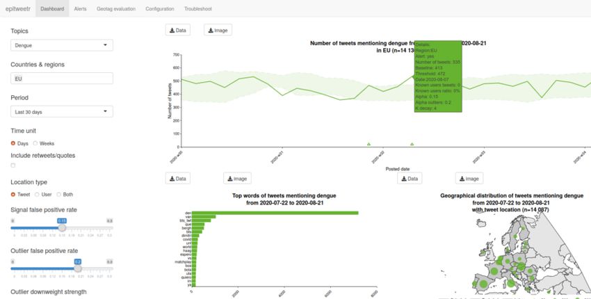
The package includes an interactive web application (Shiny app) with five pages: the dashboard, where a
user can visualise and explore tweets (Fig 1), the alerts page, where you can view the current alerts and
associated information (Fig 2), the geotag evaluation page, where you can evaluate the geolocation
algorithm in different tweet fields to manually choose the geolocation threshold (Fig 3), the configuration
page, where you can change settings and check the status of the underlying processes (Fig 4), and the
troubleshoot page, with automatic checks and hints for using epitweetr with all its functionalities (Fig 5).
On the dashboard, users can view the aggregated number of tweets over time, the location of these tweets
on a map and the words most frequently found in these tweets. These visualisations can be filtered by the
topic, location and time period you are interested in. Other filters are available and include the possibility to
adjust the time unit of the timeline, whether retweets/quotes should be included, what kind of geolocation
types you are interested in, the sensitivity of the prediction interval for the signal detection, and the number
of days used to calculate the threshold for signals. This information is also downloadable directly from this
interface in the form of data, pictures, or reports.
Shiny app dashboard:
Fig 1: Shiny app dashboard figure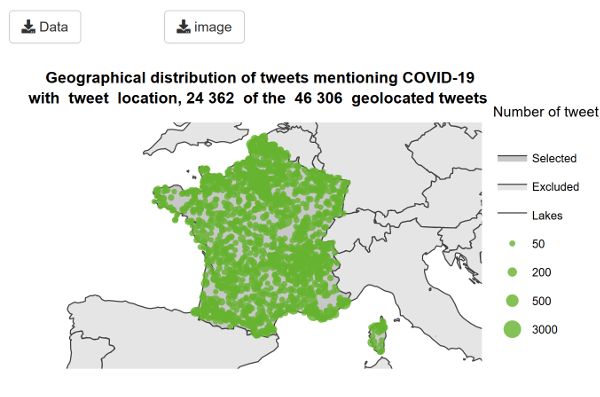
Shiny app alerts page:
                                    Fig 2: Shiny app alerts page

Shiny app geotag evaluation page:
                             Fig 3: Shiny app geotag evaluation page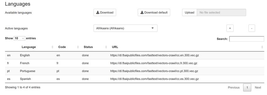
Shiny app configuration page:
                                Fig 4: Shiny app configuration page

Shiny app troubleshoot page:
                                Fig 5: Shiny app troubleshoot page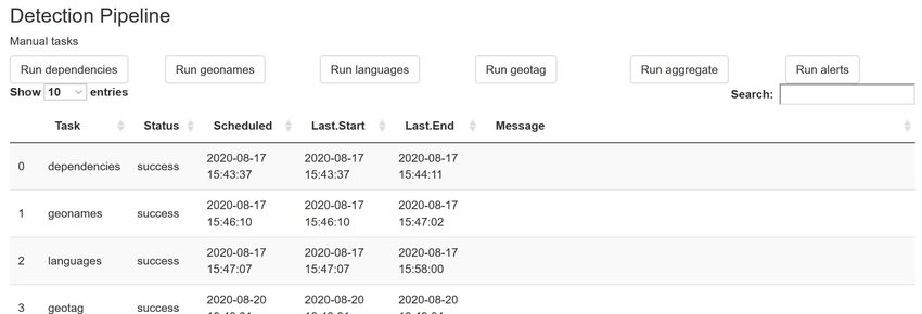
Background

Epidemic Intelligence at ECDC

Article 3 of the European Centre for Disease Prevention and Control (ECDC) funding regulation and the
Decision No 1082/2013/EU on serious cross-border threats to health have established the detection of
public health threats as a core activity of ECDC.
ECDC performs Epidemic Intelligence (El) activities aiming at rapidly detecting and assessing public health
threats, focusing on infectious diseases, to ensure EU’s health security. ECDC uses social media as part
of its sources to early detect signals of public health threats. Until 2020, the monitoring of social media was
mainly performed through the screening and analysis of posts from pre-selected experts or organisations,
mainly in Twitter and Facebook.
More information and an online tutorial are available:
EI sources
EI tutorial

Monitoring social media trends

Some signals are not detected at all or are not detected early enough by the methods explained above.
The automated monitoring of metadata from social media (e.g. analysis of social media trends) allows the
detection of signals that may not be detected by the monitoring of pre-selected accounts in social media,
and it improves the timeliness of signal detection.
The analysis of trends from social media by topic, time and place generates relevant signals for early
detection.
In 2019, ECDC developed a prototype of a manual R-based tool for the early detection of public health
threats from Twitter data. The epitweetr package is an extension of this prototype, to allow a wider
geolocation of tweets and greater automatisation.

Objectives of epitweetr

The primary objective of epitweetr is to use the Twitter Standard Search API version 1.1 in order to detect
early signals of potential threats by topic and by geographical unit.
Its secondary objective is to enable the user through an interactive Shiny interface to explore the trend of
tweets by time, geographical location and topic, including information on top words and numbers of tweets
from trusted users, using charts and tables.

Hardware requirements

The minimum and suggested hardware requirements for the computer are in the table below:

                  Hardware requirements                  Minimum Suggested

                  RAM Needed                             8GB         16GB recommended

                  CPU Needed                             4 cores     12 cores

                  Space needed for 3 years of storage 3TB            5TB

The CPU and RAM usage can be configured on the Shiny app configuration page (see section The
interactive user application (Shiny app)>The configuration page). The RAM, CPU and space needed may
depend on the amount and size of the topics you request in the collection process.

Installation

epitweetr is conceived to be platform independent, working on Windows, Linux and Mac. We recommend
that you use epitweetr on a computer that can be run continuously. You can switch the computer off, but
you may miss some tweets if the downtime is large enough, which will have implications for the alert
detection. Before using epitweetr, the following items need to be installed:

Prerequisites for running epitweetr

      R version 3.6.3 or higher
      Java 1.8 eg. openjdk version “1.8” https://www.java.com/download/. The 64-bit rather than the 32-bit
      version is preferred, due to memory limitations. In Mac, also the Java Development Kit
      https://docs.oracle.com/javase/9/install/installation-jdk-and-jre-macos.htm]
      If you are running it in Windows, you will also need Microsoft Visual C++, however in most cases it
      is likely to be pre-installed:
             Microsoft Visual C++ 2010 Redistributable Package (x64) https://www.microsoft.com/en-
             us/download/details.aspx?id=14632

Prerequisites for some of the functionalities in epitweetr

      Pandoc, for exporting PDFs and Markdown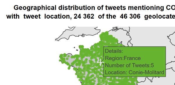
https://pandoc.org/installing.html

      Tex installation (TinyTeX or MiKTeX) (or other TeX installation) for exporting PDFs
             (easiest) https://yihui.org/tinytex/ (install from R, logoff/logon required after installation)
             https://miktex.org/download (full installation required, logoff/logon required after installation)
      Machine learning optimisation (only for advanced users)
             Open Blas (BLAS optimizer), which will speed up some of the geolocation processes:
             https://www.openblas.net/ Installation instructions: https://github.com/fommil/netlib-Java
             or Intel MKL (https://software.intel.com/content/www/us/en/develop/tools/math-kernel-
             library/choose-download.html)
      A scheduler
             If using Windows, you need to install the R package: taskscheduleR
             If using Linux, you need to plan the tasks manually
             If using a Mac, you need to install the R package: cronR

Extra prerequisites for R developers

If you would like to develop epitweetr further, then the following development tools are needed:
      Git (source code control) https://git-scm.com/downloads
      Sbt (compiling scala code) https://www.scala-sbt.org/download.html
      If you are using Windows, then you will additionally need Rtools: https://cran.r-
      project.org/bin/windows/Rtools/

External dependencies

epitweetr will need to download some dependencies in order to work. The tool will do this automatically
the first time the alert detection process is launched. The Shiny app configuration page will allow you to
change the target URLs of these dependencies, which are the following:
      CRAN JARs: Transitive dependencies for running Spark, Lucene and embedded scala code.
      [https://repo1.maven.org/maven2]
      Winutils.exe (Windows only) This is a Hadoop binary necessary for running SPARK locally on
      Windows [http://public-repo-1.hortonworks.com/hdp-win-alpha/winutils.exe].

Installing epitweetr from CRAN

After installing all required dependencies listed in the section “Prerequisites for running epitweetr”, you can
install epitweetr:

 install.packages(epitweetr)

 Environment variables

Additionally, the R environment needs to know where the Java installation home is. To check this, type in
the R console:

 Sys.getenv("JAVA_HOME")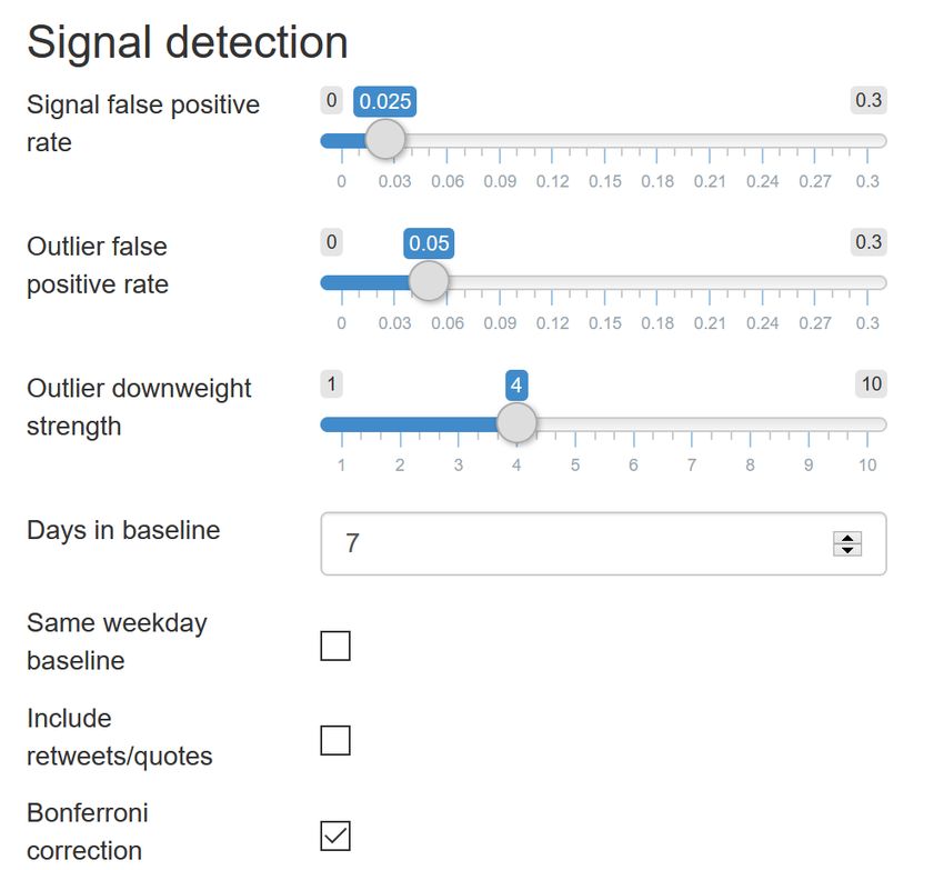
If the command returns Null or empty, then you will need to set the Java Home environment variable, for
your OS, please see your specific OS instructions. In some cases, epitweetr can work without setting the
Java Home environment variable.
The first time you run the application, if the tool cannot identify a secure password store provided by the
operating system, you will see a pop-up window requesting a keyring password (Linux and Mac). This is a
password necessary for storing encrypted Twitter credentials. Please choose a strong password and
remember it. You will be asked for this password each time you run the tool. You can avoid this by setting
a system environment variable named ecdc_twitter_tool_kr_password containing the chosen password.

 Launching the epitweetr Shiny app

You can launch the epitweetr Shiny app from the R session by typing in the R console. Replace “data_dir”
with the designated data directory which is a local folder you choose to store tweets, time series and
configuration files in:

 library(epitweetr)
 epitweetr_app("data_dir")

Please note that the data directory entered in R should have “/” instead of “" (an example of a correct path
would be ‘C:/user/name/Documents’). This applies especially in Windows if you copy the path from the File
Explorer.
Alternatively, you can use a launcher: In an executable .bat or shell file type the following, (replacing
“data_dir” with the designated data directory)
R –vanilla -e epitweetr::epitweetr_app(“data_dir”)
You can check that all requirements are properly installed in the troubleshoot page. More information is
available in section The interactive user application (Shiny app)>Dashboard:The interactive user interface
for visualisation>The troubleshoot page

Setting up tweet collection and the alert detection loop

In order to use epitweetr, you will need to collect tweets and run the alert detection loop (geonames,
languages, geotag, aggregate and alerts). Further details are also available in subsequent sections of the
user documentation. A summary of the steps needed is as follows:
      Launch the Shiny app (from the R console)

 library(epitweetr)
 epitweetr_app("data_dir")

      On the configuration page of the Shiny app, in the manual tasks of the “Detection pipeline”, click on
      “Run dependencies”, “Run geonames” and “Run languages” (their status will change to “pending”).
      This allows the detection pipeline to download the elements needed. As long as no languages are
      added and no updates are available in geonames.org, these tasks have to be run only the first time
      you install epitweetr.

      Set up the Twitter authentication using a Twitter account or a Twitter developer app, see section
      Collection of tweets>Twitter authentication for more details
      Activate the tweet collection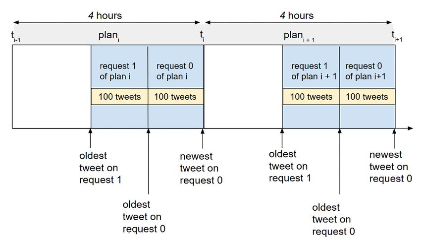
Windows: Click on the “Tweet search” activate button

            Other platforms: In a new R session run the following command

 library(epitweetr)
 search_loop("data_dir")

      You can confirm that the tweet collection is running if the “Tweet search” status is “Running” on the
      Shiny app configuration page (green text in screenshot above) and “true” in the Shiny app
      troubleshoot page.
      Activate the detection pipeline:
            Windows: Click on the “Detection pipeline” activation button

            Other platforms: In a new R session run the following command

 library(epitweetr)
 detect_loop("data_dir")

      You can confirm that the detection pipeline is running if the “Detection pipeline” status is “Running”
      in the Shiny app configuration page and “true” in the Shiny app troubleshoot page.
      You will be able to visualise tweets after the aggregate step in the detection pipeline table on the
      Shiny app configuration page is finished and if “Tweet search” is activated.
      You can start working with the generated signals. Happy signal detection!

For more details you can go through the section How does it work? General architecture behind epitweetr,
which describes the underlying processes behind the tweet collection and the signal detection. Also, the
section “The interactive Shiny application (Shiny app)>The configuration page” describes the different
settings on the configuration page.

How does it work? General architecture behind epitweetr

The following sections describe in detail the above general principles. The settings of many of these
elements can be configured in the Shiny app configuration page, which is explained in the section The
interactive Shiny application (Shiny app)>The configuration page.

Collection of tweets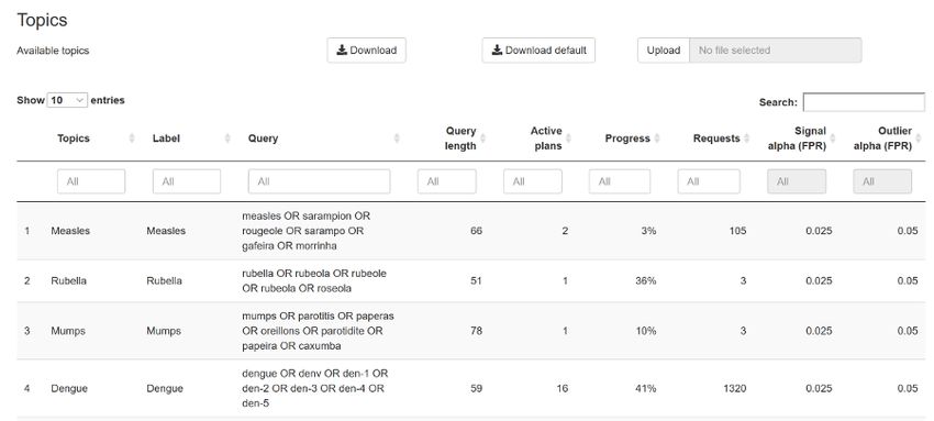
Use of the Twitter Standard Search API version 1.1

epitweetr uses the Twitter Standard Search API version 1.1. The advantage of this API is that it is a free
service provided by Twitter enabling users of epitweetr to access tweets free of charge. The search API is
not meant to be an exhaustive source of tweets. It searches against a sample of recent tweets published in
the past 7 days and it focuses on relevance and not completeness. This means that some tweets and
users may be missing from search results.
While this may be a limitation in other fields of public health or research, the epitweetr development team
believe that for the objective of signal detection a sample of tweets is sufficient to detect potential threats
of importance in combination with other type of sources.
Other attributes of the Twitter Standard Search API version 1.1 include:
      Only tweets from the last 5–8 days are indexed by Twitter
      A maximum of 180 requests every 15 minutes are supported by the Twitter Standard Search API
      (450 requests every 15 minutes if you are using the Twitter developer app credentials; see next
      section)
      Each request returns a maximum of 100 tweets and/or retweets

 Twitter authentication

You can authenticate the collection of tweets by using a Twitter account (this approach utilises the rtweet
package app) or by using a Twitter application. For the latter, you will need a Twitter developer account,
which can take some time to obtain, due to verification procedures. We recommend using a Twitter
account via the rtweet package for testing purposes and short-term use, and the Twitter developer
application for long-term use.
      Using a Twitter account: delegated via rtweet (user authentication)
             You will need a Twitter account (username and password)
             The rtweet package will send a request to Twitter, so it can access your Twitter account on
             your behalf
             A pop-up window will appear where you can enter your Twitter user name and password to
             confirm that the application can access Twitter on your behalf. You will send this token each
             time you access tweets.
      Using a Twitter developer app: via epitweetr (app authentication)
             If you have not done so already, you will need to create a Twitter developer account:
             https://developer.twitter.com/en/apply-for-access
             Create an app
             For the access type, ensure you have read and write access
             Make a note of your OAuth settings
                    Add them to the configuration page in the Shiny app (see image below)
                    With this information epitweetr can request a token at any time directly to Twitter. The
                    advantage of this method is that the token is not connected to any user information and
                    tweets are returned independently of any user context.
                    With this app you can perform 450 requests every 15 minutes instead of the 180
                    requests every 15 minutes that a Twitter account allows.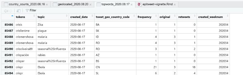
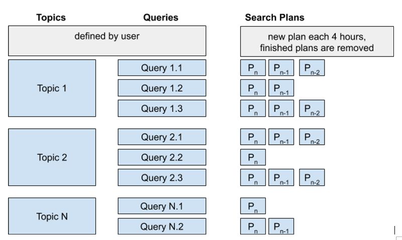
Topics and tweet collection queries

After the Twitter authentication, you need to specify a list of topics in epitweetr to indicate which tweets to
collect. For each topic, you have one or more queries that epitweetr uses to collect the relevant tweets
(e.g. several queries for a topic using different terminology and/or languages).
A query consists of keywords and operators that are used to match tweet attributes. Keywords separated
by a space indicate an AND clause. You can also use an OR operator. A minus sign before the keyword
(with no space between the sign and the keyword) indicates the keyword should not be in the tweet
attributes. While queries can be up to 512 characters long, best practice is to limit your query to 10
keywords and operators and limit complexity of the query, meaning that sometimes you need more than
one query per topic.
epitweetr comes with a default list of topics as used by the ECDC Epidemic Intelligence team at the date
of package generation (1st of September, 2020). You can view details of the list of topics in the Shiny app
configuration page (see screenshot below).

On the configuration page, you can also download the list of topics, modify it and upload it to epitweetr.
The new list of topics will then be used for tweet collection and visible in the Shiny app. The list of topics is
an Excel file (*.xlsx) as it handles user-specific regional settings (e.g. delimiters) and special characters
well. You can create your own list of topics and upload it too, noting that the structure should include at
least:
      The name of the topic, with the header “Topic” in the Excel spreadsheet. This name should include
      alphanumeric characters, spaces, dashes and underscores only. Note that it should start with a
      letter.
The query, with the header “Query” in the Excel spreadsheet. This is the query epitweetr uses in its
requests to obtain tweets from the Twitter Standard Search API. See above for syntax and
constraints of queries.
The topics.xlsx file additionally includes the following fields:
An ID, with the header “#” in the Excel spreadsheet, noting a running integer identifier for the topic.
A label, with the header “Label” in the Excel spreadsheet, which is what is displayed in the drop-
down topic menu of the Shiny app tabs.
An alpha parameter, with the header “Signal alpha (FPR)” in the Excel spreadsheet. FPR stands for
“false positive rate”. Increasing the alpha will decrease the threshold for signal detection, resulting in
an increased sensitivity and possibly obtaining more signals. Setting this alpha can be done
empirically and according to the importance and nature of the topic.
“Length_charact” is an automatically generated field that calculates the length of all characters used
in the query. This field is helpful as a request should not exceed 500 characters.
“Length_word” indicates the number of words used in a request, including operators. Best practice is
to limit your number of keywords to 10.
An alpha parameter, with the header “Outlier alpha (FPR)” in the Excel spreadsheet. FPR stands for
“false positive rate”. This alpha sets the false positive rate for determining what an outlier is when
downweighting previous outliers/signals. The lower the value, the fewer previous outliers will
potentially be included. A higher value will potentially include more previous outliers.
“Rank” is the number of queries per topic
When uploading your own file, please modify the topic and query fields, but do not modify the column
titles.
Scheduled plans to collect tweets
As a reminder, epitweetr is scheduled to make 180 requests (queries) to Twitter every 15 minutes (or 450
requests every 15 minutes if you are using Twitter developer app credentials). Each request can return
100 tweets. The requests return tweets and retweets. These are returned in JSON format, which is a light-
weight data format.
In order to collect the maximum number of tweets, given the Standard Search API limitations, and in order
for popular topics not to prevent other topics from being adequately collected, epitweetr uses “search
plans” for each query.
The first “search plan” for a query will collect tweets from the current date-time backwards until 7 days (7
days because of the Standard Search API limitation) before the current “search plan” was implemented.
The first “search plan” is the biggest, as no tweets have been collected so far.
All subsequent “search plans” are scheduled intervals that are set up in the configuration page of the
epitweetr Shiny app (see section The interactive Shiny app > the configuration page > General). For
illustration purposes, let us consider the search plans are scheduled at four-hour intervals. The plans
collect tweets for a specific query from the current date-time back until four hours before the date-time
when the current “search plan” is implemented (see image below). epitweetr will make as many requests
(each returning up to 100 tweets) during the four-hour interval as needed to obtain all tweets created within
that four-hour interval.
For example, if the “search plan” begins at 4 am on the 10th of September 2020, epitweetr will launch
requests for tweets corresponding to its queries for the four-hour period from 4 am to midnight on the 10th
of September 2020. epitweetr starts by collecting the most recent tweets (the ones from 4 am) and
continues backwards. If during the four-hour time period between 4am and midnight the API does not
return any more results, the “search plan” for this query is considered completed.However, if topics are very popular (e.g. COVID-19 in 2020), then the “search plan” for a query in a given
four-hour window may not be completed. If this happens, epitweetr will move on to the “search plans” for
the subsequent four-hour window, and put any previous incomplete “search plans” in a queue to execute
when “search plans” for this new four-hour window are completed.
Each “search plan” stores the following information:
Field Type Description
expected_end Timestamp End DateTime of the current search window
The scheduled DateTime for the next request. On plan creation this will be
the current DateTime and after each request this value will be set to a future
scheduled_for Timestamp DateTime. To establish the future DateTime, the application will estimate the
number of requests necessary to finish. If it estimates that N requests are
necessary, the next schedule will be in 1/N of the remaining time.
start_on Timestamp The DateTime when the first request of the plan was finished
The DateTime when the last request of the plan was finished if that request
end_on Timestamp
reached a 100% plan progress.
The max Twitter id targeted by this plan, which will be defined after the first
max_id Long
request
The last tweet id returned by the last request of this plan. The next request
since_id Long will start collecting tweets before this value. This value is updated after each
requests and allows the Twitter API to return tweets before min_time(pi)
If a previous plan exists, this value stores the first tweet id that was
since_target Long downloaded for that plan. The current plan will not collect tweets before that
id. This value allows the Twitter API to return tweets after pi-time_back
requests Int Number of requests performed as part of the plan
Progress of the current plan as a percentage. It is calculated as
(current$max_id - current$since_id)/(current$max_id -
progress Double current$since_target). If the Twitter API returns no tweets the progress is set
to 100%. This only applies for non error responses containing an empty list
of tweets.
epitweetr will execute plans according to these rules:epitweetr will detect the newest unfinished plan for each search query with the scheduled_for
variable located in the past.
epitweetr will execute the plans with the minimum number of requests already performed. This
ensures that all scheduled plans perform the same number of requests.
As a result of the two previous rules, requests for topics under the 180 limit of the Twitter Standard
Search API (or 450 if you are using Twitter developer app authentication) will be executed first and
will produce higher progress than topics over the limit.
The rationale behind this is that topics with such a large number of tweets that the 4-hour search window is
not sufficient to collect them, are likely to already be a known topic of interest. Therefore, priority should be
given to smaller topics and possibly less well-known topics.
An example is the COVID-19 pandemic in 2020. In early 2020, there was limited information available
regarding COVID-19, which allowed detecting signals with meaningful information or updates (e.g. new
countries reporting cases or confirming that it was caused by a coronavirus). However, throughout the
pandemic, this topic became more popular and the broad topic of COVID-19 was not effective for signal
detection and was taking up a lot of time and requests for epitweetr. In such a case it is more relevant to
prioritise the collection of smaller topics such as sub-topics related to COVID-19 (e.g. vaccine AND
COVID-19), or to make sure you do not miss other events with less social media attention.
If search plans cannot be finished, several search plans per query may be in a queue:
Geolocation
In a parallel process to the collection of tweets, epitweetr attempts to geolocate all collected tweets using
an unsupervised machine learning process. This process runs in the schedule window defined by “Detect
span” property in the configuration page under “General settings” (e.g. if a four-hour window is set it will
run every four hours and will geolocate all tweets collected since the last time it successfully ran).
epitweetr stores two types of geolocation for a tweet: tweet location, which is geolocation information
within the text of a tweet (or a retweeted or quoted tweet), and user location from the available metadata.
For signal detection, the best location is used while in the dashboard both types can be visualised.
Geolocation based on tweet location
The tweet location is extracted and stored by epitweetr based on the geolocation information found within
a tweet text. In case of a retweet or quoted tweet, it will extract the geolocation information from the
original tweet text that was retweeted or quoted. If neither is available, no tweet location is stored based on
tweet text.epitweetr identifies if a tweet text contains reference to a particular location by breaking down the tweet
text into sets of words and evaluating those which are more likely to be a location by using a machine
learning model. The algorithm also adds further words (one by one) to the set and if the score grows by
using more words, the algorithm tries to find a local maximum of the score with a bigger text. It then
matches these words against a reference database, which is geonames.org. This is a geographical
database available and accessible through various web services, under a Creative Commons attribution
license. The GeoNames.org database contains over 25,000,000 geographical names. epitweetr uses by
default those limited to currently existing ones and those with a known population (so just over 500,000
names). You can override this default on the Shiny app configuration page, by unchecking “Simplified
geonames”. The database also contains longitude and latitude attributes of localities and variant spellings
(cross-references), which are useful for finding purposes, as well as non-Roman script spellings of many of
these names.
The matches can be performed at any level of administrative hierarchy. The matching is powered by
Apache Lucene, which is an open-source high-performance full-featured text search engine library.
Some text may have several locations through the matching process. However, only the location with the
highest score will be selected.
A higher score is associated with a greater probability that a match is correct. A score is:
Higher if unusual parts of the name are matched
Higher if several administrative levels are matched
Higher if location population is bigger
Higher for countries and cities vs administrative levels
Higher for capital letter acronyms like NY
Lower for words that are more likely to be other (non-geographical) kinds of words. For example
“Fair Play” town in Colorado. This is achieved by using language models provided by fasttext.cc.
You can select which languages you would like to check for other kinds of words in, by selecting the active
language desired within the configuration page of the Shiny app and clicking on the “+” icon:
In addition, you can unselect languages by selecting the language within the configuration page of the
Shiny app and clicking on the “-” icon: ADD IMAGE HERE
A minimum score (the “geolocation threshold”) can be globally set in the general settings on the
configuration page to reduce the number of false positives (see image). All geolocations with a smaller
score than the geolocation threshold will be discarded by the algorithm as tweet location. If there is more
than one match over the minimum score, then the match with the highest score will be chosen.
The threshold is empirically chosen and can be evaluated against a human read of tweets and tweet
locations, on the geotag evaluation page.Geolocation based on user location
Different types of user locations are available from the metadata provided through the Twitter Standard
Search API. epitweetr selects the best user location for the aggregated files using the following order:
the user’s exact or approximate location at time of the tweet (provided by the API)
if the user’s location is not available and the tweet is a retweet or a quoted tweet, then the user’s
exact or approximate location at time of the retweet/quoted tweet is used (provided by the API)
if not available, then the user declared location is used
if not available, then the “home” in the public profile is used.
With exact locations, the longitude and latitude are provided. If it is the estimated location, epitweetr
calculates the longitude and latitude from GeoNames.org.
If user location information provided by the API is not available, then epitweetr will calculate longitude and
latitude from the user declared location or the place name given in the user “public profile”, using
GeoNames.org.
Stored geolocated tweet information
The geolocation of the match is stored as a country code (using the ISO 3166 standard) and a longitude
and latitude associated with the exact geolocation in the aggregated data.
Most frequent words found in tweets
As the number of tweets and words can be very large, tweets are analysed for most frequent words in
chunks of 10 000 tweets to get the top 500 words of each chunk for the same language, day and topic.
To ensure reasonable performance of epitweetr, the 500 top words are first determined globally, and then
these words are used to subset by country, to get the top words by country, day and topic. In very small
locations with few number of tweets geolocated, there may be no frequent words available.
Note that, differently to the other visualisation figures, the most frequent words in tweets are always based
on the geolocation related to “tweet location” and not to “user location” regardless of the filter selected in
the dashboard.
Aggregation of data
The aggregation process produces three Rds files (a native R format): geolocated, country_counts and
topwords.In the geolocated Rds file, the number of tweets or retweets are stored by topic, date, tweet text geolocation longitude and latitude and user geolocation longitude and latitude. Each of these entries also has the country associated with the tweet text geolocation and the country associated with the user geolocation (see partial screenshot below). Note that tweets without geolocation information are also included. The country_counts Rds file is used to create the trendline in the Shiny app. This is a smaller Rds file, without the longitude and latitude information, and includes the number of tweets by hour within a day, by country (according to tweet location or user location), topic (see screenshot), and whether a tweet was a retweet or not. The known_retweets and known_original fields give the number of tweets or retweets from a list of “important users”. In this file, tweets without geolocation are also included. Including tweets without geolocation information enables you to view all tweets when selecting “world” as a region, regardless if geolocation was successful or not. The aggregation by top words is stored in the topwords.Rds file, and displays the number of tweets or retweets (or both) by topic, top word, date, country of tweet location and whether a tweet was a retweet or not (see screenshot). Signal detection The main objective of epitweetr is to detect signals in the observed data streams, i.e. counts in the aggregated time series that exceed what is expected. For detecting signals, epitweetr uses an extended version of the EARS (Early Aberration Reporting System) algorithm (Fricker, Hegler, and Dunfee 2008), which in what follows is denoted by eears (extended EARS). This algorithm is part of the R package surveillance (Salmon, Schumacher, and Höhle 2016). As a default it uses a moving window of the past seven days to calculate a threshold. If the count for the current day exceeds this threshold, then a signal is generated. Details of the algorithm underlying signal detection
The eears algorithm is applied on the counts from the past seven 24-hour blocks prior to the current 24
hour block of the signal detection. The running mean and the running standard deviation are calculated:

                                        −1                                       −1
                                    1                                     1                     2
                                                                 2
                         ¯¯                                                              ¯¯
                         ȳ 0
                                =       ∑ yt          and    s       =           ∑ (yt − ȳ 0
                                                                                              ) ,
                                                                 0
                                    7                                    7 − 1
                                        t=−7                                     t=−7

where yt , t = … , −2, −1, 0 denotes the observed count data time series with time index 0 denoting the
current block. Furthermore, the time index −7, … , −1 denote the seven blocks prior to the current block.
Under the null hypothesis of no spikes, it is assumed that the yt are identically and independently
N (μ, σ ) distributed with unknown mean μ and unknown variance σ . Hence, the upper limit of a simple
       2                                                                2

one-sided (1 − α)× 100% plug-in prediction interval for y0 based on y−7 , … , y−1 is given as

                                                         ¯¯
                                                    U0 = ȳ 0
                                                              + z 1−a × s0 ,

where z1−a is the (1 − α)- quantile of the standard normal distribution. An alert is raised if y0 > U0 . If one
uses α=0.025, then this corresponds to investigating, if y0 exceeds the estimate for the mean plus 1.96
times the standard deviation. However, as pointed out by Allévius and Höhle (2017), the correct approach
would be to compare the observation to the upper limit of a two-sided 95% prediction interval for y0 ,
because this respects both the sampling variation of a new observation and the uncertainty originating
from the parameter estimation of the mean and variance. Hence, the statistical appropriate form is to
compute the upper limit by
                                                                                      −−−−−
                                                                                          1
                                    U0 =   ¯¯¯¯¯¯
                                             y0     + t1−a (7 − 1) × s0 × √ 1 +             .
                                                                                          7

where t1−a (k − 1) denotes the 1 − α quantile of the t-distribution with k − 1 degrees of freedom.

 Downweighting previous signals

If previous signals are included without modification in the historic values when calculating the running
mean and standard deviation for the signal detection, then the estimated mean and standard deviation
might become too large. This may mean that important current signals will not be detected. To address this
issue, epitweetr downweights previous signals, such that the mean and standard deviation estimation is
adjusted for such outliers using an approach similar to that used in the C. P. Farrington et al. (1996).
Historic values that are not identified as previous signals are given a weight of “1”. Similarly, historic values
identified as signals are given a weight lower than one and a new fit is performed using these weights
(scaled s.t. they again sum to 7 observations). Details on the downweighting procedure can be found in
Annex I of this user documentation.

 Timing of signal detection

Signal detection is carried out based on “days”, which are moving windows of 24 hours, moving according
to the detect span (see also section The interactive user application (Shiny app) > The configuration page
> General). The baseline is calculated on these “days” from -1 to -8 (if the current “day” is zero).
Signals are generated according to the detect span (see section The interactive user application (Shiny
app) > The configuration page > General), with
      general email alerts either following this detect span (e.g. if the detect span was four hours, the
      email alerts will be sent every four hours)
      email alerts in real-time. In these email alerts, previously generated signals will be omitted.

The different types of email alerts for each user can be specified in the configuration page (see section
The interactive user application (Shiny app) > The configuration page > General).

 The alpha parameter: the false positive rate of the signal detection
A key attribute of signal detection is the ability of an algorithm to detect true threats or events without
overloading the investigators with too many false positives. In this way, the alpha parameter determines
the threshold of the detection interval. If the alpha is high, then more potential signals are generated and if
the alpha is low fewer potential signals are generated (but potential threats or events could be missed).
The setting of the alpha is often done empirically, and depends also on the resources of those
investigating the signals and the importance of missing a potential threat or event.
There is a global alpha, that can be set/changed in the epitweetr configuration page under “Signal false
positive rate” (see section The interactive user application (Shiny app) > The configuration page >
General). Additionally, the default alpha can be overridden in the topics list. Here, if you like, you can
associate each topic with a specific alpha, depending on the estimated public health importance of the
topic or potential associated event or threat.
Bonferroni correction
To account for multiple testing, for country-specific signal detection, as a default, the alpha is divided by
the number of countries. For continent-specific signal detection, the alpha is divided by the number
continents. This is a Bonferroni correction for multiple testing.
To override this, you can uncheck “Bonferroni correction” in the “Signal detection” part of the configuration
page in the Shiny app.
Using same weekdays as baseline
It is possible that there is a “day of the week effect”, where more tweets may be tweeted on a given day of
the week (e.g. Monday) than on other days. To avoid this, you can also choose to calculate the baseline
not on consecutive days, but on the past N days that correspond to the same 24 hour window N days
back. This way if N = 7, the baseline is calculated using the “days” from -7, -14, -21, -28, -35, -42, -49 and
-56 (if the current “day” is zero).
This option is on the configuration page of the Shiny app “Default same weekday baseline”.
Sending email alerts
Emails containing a list of signals detected are sent automatically by epitweetr according to the detect
span and the subscribers list. Due to the time necessary to collect, geolocate and aggregate the tweets,
email alerts will miss the most recent tweets that have not yet gone to these processes. The lag between
tweets and alerts is expected to be less than (2 * ( collect_span ) + detect_span) which should be 3h30
using default values.
The email alerts will include the following information on the signals for each topic:
The date and hour the signal was detected
The geographical location(s) where the signal was detected
The most frequent words (top words) in the tweets
The number of tweets and the threshold
The percentage of tweets from important users
Information on the settings, such as: was the Bonferroni correction used, was the same weekday
baseline used, were retweets included, etc.
This information is also available in the alerts page of the Shiny app.
The subscribers can receive real-time alerts (i.e. as soon as the detection loop is finalised) or scheduled
alerts (e.g. once or twice a day). The subscribers list can be changed in the configuration page by
downloading the Excel spreadsheet. This file has the following variables:
“User”: name of the subscriber (e.g. Jane Doe).
“Email”: email of the subscriber (e.g. jane.doe@email.com).“Topics”: list of topics for which the subscriber will receive scheduled alerts. The names used must
match the column “Topic” in the list of topics.
“Excluded”: topic for which the subscribers will not receive scheduled alerts.
“Real time Topics”: list of topics for which the subscriber will receive real-time alerts.
“Regions”: list of regions for which the subscriber will receive scheduled alerts.
“Real time Regions”: list of regions for which the subscriber will receive real-time alerts.
“Alert Slots”: these are the detection loop slots after which the subscriber will receive the scheduled
alert. Available slots can be taken from “Launch slots” in the “General” section of the configuration
page. If no value is included, the subscriber will receive real-time alerts for all topics and regions,
even if there are real-time topics or regions specified in the Excel spreadsheet.
When including more than one topic and/or region in the subscribers list, these should be separated by
semi-colon (;) with no spaces (e.g. Ebola;infectious diseases;dengue). The names must match the column
“Topics” in the list of topics and the column “Name” in the contry/region list from the configuration page.
Folder structure
epitweetr stores tweets, aggregated tweets and the configuration in the “data folder” you have to
designate when launching the application.
Within the data folder there are 3 JSON files:
properties.json, generated from the information from the General properties of the Shiny app
topics.json managed by the search loop: it keeps a track of tweet collection plans and progress
tasks.json managed by the detect loop: it keeps information and status of the different tasks done by
this process.
There are also the following subfolders:
“geo”, which stores the GeoNames data as text and index files
“hadoop”, which stores Spark dependencies for Windows operating systems
“jars”, where collections of Java dependencies are stored that are needed in the geolocation and
aggregate processes
“languages”, where the fasttext files indexes and models are stored that are used to perform
geolocation in the tweet text
“stats”, where json files are stored reporting statistics used to optimise the aggregate process by
linking tweet files and posted dates of tweets
“alerts” that store json files of alerts detected by the detect loop.
“tweets” and “series” that are explained in more detail below.
Data folder > tweets
In the data folder, the subfolder “tweets” has two further subfolders: search and geolocated
The search folder contains subfolders for each topic listed in the topics list:Within each of these topics you have a year (e.g. 2020) and then a compressed json file containing the
tweets by day for each year. The dates pertain to the dates the tweet was collected (not tweeted). There
may be more than one file for one day if the file exceeds 100 MB.
The geolocated folder contains compressed json files with geolocated information produced by the
geolocated algorithm.
Data folder > series
In the series folder, epitweetr stores the aggregated data of the geolocated tweets as well as the top
words.
There is a folder for each ISO week of date of collection containing Rds files (a native R format file) for
each day and series:
geolocated_YYY.MM.DD.Rds contains daily tweet counts at finest possible location level
topwords_YYY.MM.DD.Rds contains daily tweet top words counts at country level
country_counts_YYY.MM.DD.Rds contains hourly tweet counts at country level
This is the aggregate information as described in the section “How does it work? General architecture of
epitweetr > Aggregation”.The interactive user application (Shiny app)
You can launch the epitweetr interactive user application (Shiny app) from the R session by typing in the R
console (replace “data_dir” with the desired data directory):
epitweetr_app("data_dir")
Alternatively, you can use a launcher: In an executable bat or sh file put the following content, (replacing
“data_dir” with the expected data directory)
R –vanilla -e epitweetr::epitweetr_app(‘data_dir’)
The epitweetr interactive user application has five pages:
The dashboard, where a user can visualise and explore tweets
The configuration page, where you can change settings and check the status of the underlying
processes
The alerts page, where you can view the current alerts and associated information
The geotag evaluation page, where you can evaluate the geolocation algorithm in different tweet
fields to manually choose the geolocation threshold
The troubleshoot page, with with automatic checks and hints for using epitweetr with all its
functionalities
Dashboard: The interactive user interface for visualisation
The dashboard is where you can interactively explore visualisations of tweets. It includes a line graph
(trend line) with alerts, a map and top words of tweets for a given topic. Please note that the first time a
period is selected, you will need to wait 1-2 minutes until you see the outputs. Likewise, for any new
selection (adding a region, changing topic, etc), epitweetr will start reading the corresponding data; so if
several selections are done, you may need to wait 1-2 minutes until the last selection is shown in the
dashboard. When epitweetr is reading new data, the outputs have less intensity giving you an indication
that new data is being read and plotted.
In order to interactively explore the data, you can select from several filters, such as topics, countries and
regions, time period, time unit, signal confidence and days in baseline.
Note that whatever options/settings you select on the dashboard, will have no effect on the alert detection.
The alert detection settings are all selected on the configuration page of the Shiny app.
Filters
Topics
You can select one item from the drop-down list of topics, which is populated by what is specified in the
topics on the configuration page. You can also start typing in the text field and select the topics from the
filtered dropdown list.
Countries & regionsIf you select World (all), all tweets are displayed regardless of their geolocation. You can select an individual country, you can select regions and subregions, and you can select several items at the same time. You can also start typing in the text field and select the geographical item from the drop-down list. Period You can select from the past 7 (the default), 30, 60 or 180 days. You can also select “custom” and a calendar option to select study period will appear. These periods will be the time period for inclusion in the visualisations. When selecting custom period, please ensure that the first date is at least one day before the second date. Time unit You can display the timeline for the number of tweets with weeks or days as units of time. The default is days. Include Retweets/quotes By default, retweets are not included in any of the visualisations. If “include retweets/quotes” is checked, the visualisations display results of tweets and retweets/quotes. Otherwise, the visualisations display only tweets (without retweets/quotes). Location type
Tweets are geolocated into regions, subregions and countries. “Location type” indicates what should be
used for geolocation:
      Tweet: this comprises geographical information contained within the tweet text or if not available,
      geographical information contained within the retweet/quoted text, if applicable.
      User: this is geographical information obtained from the user location. In order of priority, this is the
      user’s location at time of the tweet, the user’s API location or the “home” in the public profile if none
      of these is available.
      Both: the geographical information used for a tweet will be, in order of priority, the location within the
      tweet text, but if not available the user location.

Signal detection false positive rate

Using the slider, you can explore the differences in the signals generated when changing the alpha
parameter for the false positive rate. Note that this will not change the signal false positive rate for the alert
emails. This is just a tool for the user to explore this parameter. The default is 0.025. A higher false positive
rate will increase the sensitivity and possibly the number of signals detected, and vice versa.
Outlier false positive rate and outlier downweight strength

The outlier false positive rate relates to the false positive rate for determining what an outlier is when
downweighting previous outliers/signals. The lower the value, the fewer previous outliers will potentially be
included. A higher value will potentially include more previous outliers.
The outlier downweight strength determines how much an outlier will be downweighted by. The higher the
value the greater the downweighting. For more information please see Annex I.
Bonferroni correction

The Bonferroni correction is selected by default. It accounts for false positive signal detection through
multiple testing. For country-specific signal detection, the alpha is divided by the number of countries. For
continent-specific signal detection, the alpha is divided by the number continents.
If you do not wish to use this correction, you can uncheck it.
Days in baseline
The default days in baseline is 7. The user can explore the effect of having different days in the baseline. This is only for the visualisation, any changes made for the email alerts have to be made in the configuration page. Same weekday baseline It is possible that there is a “day of the week effect”, where more tweets may be tweeted on a given day of the week (e.g. Monday) than on other days. You can also select to calculate the baseline not on consecutive days, but on the past N days that correspond to the same 24 hour window N days back. This way if N = 7, the baseline is calculated using the “days” from -7, -14, -21, -28, -35, -42, -49 and -56 (if the current “day” is zero). The timeline The timeline graph is a time series, where you can see the number of tweets for a given topic, geographical unit and study period. Signals are indicated as triangles on the graph, with the alpha and baseline days as specified in the filters. The area under the threshold is indicated in the shaded green colour. Note that the signals are related to the choice of alpha and days in baseline in the filters on the dashboard, rather than what is used for the alert emails. This way you can explore the effect of changing these parameters and adapt the settings for the alert emails if needed. If you hover over the graph, you obtain extra information on country, date, number of tweets and the number of tweets from the list of known users, the ratio of known users to unknown users, whether the number of tweets was associated with a signal and what the threshold and the alpha was. Map
The map shows a proportional symbol map of the tweets by country and by topic for the study period. The
larger the circle, the greater the number of tweets.
The geographical information for the map is based on the choice in the filters: the country/region/subregion
and the location type (tweet, user or both).

When you hover over the map, you can get information on number of tweets and names of the
geographical units underlying the circles on the map.
When selecting one country, the symbols show the geographical distribution of tweets at subnational level.
When selecting two or more countries or other geographical entity (e.g. regions or continents), the symbols
show the geographical distribution of tweets at national level. Note that if a tweet has a geotag at country
level (e.g. France), it will not be displayed when selecting only that country since no subnational
geotagging is available.

 Most frequent words found in tweets

Tweets are analysed globally to get the top 500 words of each chunk for the same language, day and
topic. These 500 words are then subsetted by country.
This graph then displays the top words of tweets by topic for the study period for the geographical units
chosen, and according to the filter on tweet/retweet.
Note that, differently to other visualisation figures, the most frequent words found in tweets is always
related to “tweet location” and is not influenced by the filter option for choice of location (user or tweet
location).

The alerts page

The alerts page summarises the signals detected within the specified study period. This summary includes
the date, hour, topic and geographical unit of the signal, which top words are included, the number of
tweets, the number of tweets from important users and the threshold. It additionally includes many of the
settings specified in the configuration page, which were used for detecting signals. This is also the output
received in the emails alerts.

The geotag evaluation page

This page supports the user in establishing the geolocation threshold in the configuration page. The user
can choose the field of the tweets to test and the number of tweets to sample. This page is for visualization
only and no changes in the geolocation detected by epitweetr is allowed.
The configuration page

In the configuration page, you can change settings of the tool, you can check the status of the various
processes/pipelines of the tool and you can add, delete and modify topics and their associated requests,
languages for geolocation and the list of the “important users” and email alert subscribers. When changing
anything in the “Signal detection” or “General” sections, do not forget to click on the “Update Properties”
button at the end of the “General” section. The following sections describe the configuration page in more
detail.

Status
The status section enables you to quickly assess the latest time point and/or status of the processes for
tweet collection (Tweet Search), and geolocation, aggregation and signal detection (Detection pipeline).
In the status section, you can tell if both the search pipeline and the detect pipeline processes are running.
If you are running Windows, you can click on “activate” to register these processes as scheduled tasks and
run them manually from the Windows task scheduler.
Detection pipeline
In the manual tasks in the “Detection pipeline”, you have. You need to run manually the tasks of
dependencies, geonames and languages by clicking in the buttons “Run dependencies”, “Run geonames”
and “Run languages” the first time you use epitweetr, and then only if you are downloading new versions.
Geonames and languages relate to the geolocation and language models used by epitweetr. If you would
like to update them (this is not something that needs to be done regularly, more on a yearly basis or so),
then you can click on “Run”.
The “Run geotag”, “Run aggregate” and “Run alerts” buttons can be used to force the start of these tasks
in case there is any error or issue. You can check their status in the “Detection Pipeline” table.
The detection pipeline gives more information about the status of the processes of epitweetr. This is useful
for troubleshooting any issues arising and monitoring progress. It contains the five tasks that are running in
the background. Geoames and languages are tasks that will download and update the local copies of
these. This will only be triggered if we add a language or update GeoNames. The start and end dates will
generally be much older than those of geotag, aggregate and alerts.
Geotag, aggregate and alerts dates should be more recent if the search and detection pipelines are active
and running. They are scheduled according to the detect span. The status can include running, scheduled,
pending, failed or aborted (if it has failed more than three times).

Signal detection
In the signal detection section in the configuration page, you can set the signal false positive rate alpha
parameter, which increases (if larger) the the detection interval (more signals are detected), or decreases
(if smaller) the detection interval (fewer signals are detected).

The outlier false positive rate relates to the false positive rate for determining what an outlier is when
downweighting previous outliers/signals. The lower the value, the fewer previous outliers will potentially be
included. A higher value will potentially include more previous outliers.
You can also read