Not Arbitrary, Systematic! Average-Based Route Selection for Navigation Experiments - Schloss ...
←
→
Page content transcription
If your browser does not render page correctly, please read the page content below
Not Arbitrary, Systematic! Average-Based Route
Selection for Navigation Experiments
Bartosz Mazurkiewicz
TU Wien, Austria
bartosz.mazurkiewicz@geo.tuwien.ac.at

Markus Kattenbeck
TU Wien, Austria
markus.kattenbeck@geo.tuwien.ac.at

Peter Kiefer
ETH Zurich, Switzerland
pekiefer@ethz.ch

Ioannis Giannopoulos
TU Wien, Austria
igiannopoulos@geo.tuwien.ac.at

      Abstract
While studies on human wayfinding have seen increasing interest, the criteria for the choice of the
routes used in these studies have usually not received particular attention. This paper presents a
methodological framework which aims at filling this gap. Based on a thorough literature review
on route choice criteria, we present an approach that supports wayfinding researchers in finding a
route whose characteristics are as similar as possible to the population of all considered routes with
a predefined length in a particular area. We provide evidence for the viability of our approach by
means of both, synthetic and real-world data. The proposed method allows wayfinding researchers
to justify their route choice decisions, and it enhances replicability of studies on human wayfinding.
Furthermore, it allows to find similar routes in different geographical areas.

2012 ACM Subject Classification Information systems → Geographic information systems; Inform-
ation systems → Location based services; Information systems → Decision support systems; General
and reference → Empirical studies

Keywords and phrases Route Selection, Route Features, Human Wayfinding, Navigation, Experi-
ments, Replicability

Digital Object Identifier 10.4230/LIPIcs.GIScience.2021.I.8

 1      Introduction
Selecting a route for a human wayfinding study in a systematic manner is a non-trivial
task. Despite its potential impact on the results, reasonable justifications for routes based
on their features are often neglected. In this paper, we propose, implement and evaluate a
methodological framework which enables researchers to choose a route for human wayfinding
experiments in a given area according to predefined, weighted criteria. The determined
routes are – with respect to these criteria – representative for a (weighted) average route for
the chosen area. Using this framework will, therefore, lead, among others, to an increased
comparability and replicability of in-situ wayfinding studies.
    Starting with the replication crisis in psychology [34], reproducibility and replicability
have both seen increased interest in all subfields of geographical sciences in recent years (see
e.g., [32, 35, 20, 24]). At the same time, studies which aim to understand human wayfinding
and/or how interactive assistance can be provided to wayfinders have gained momentum
[21, 12]. These research efforts will likely be continued in the future, as there is neither a
            © Bartosz Mazurkiewicz, Markus Kattenbeck, Peter Kiefer, and Ioannis Giannopoulos;
            licensed under Creative Commons License CC-BY
11th International Conference on Geographic Information Science (GIScience 2021) – Part I.
Editors: Krzysztof Janowicz and Judith A. Verstegen; Article No. 8; pp. 8:1–8:16
                   Leibniz International Proceedings in Informatics
                   Schloss Dagstuhl – Leibniz-Zentrum für Informatik, Dagstuhl Publishing, Germany
8:2 Systematic Route Selection
general agreement on algorithms nor route descriptions or an anywhere close to definite
understanding of the interplay between spatial cognition and the assistance provided by
mobile navigation companions. While there has been some recent progress in terms of
reproducibility (i.e., software and data are made available to the scientific community and
rerunning the analysis using the software and data yields the published results, see [6]), e.g.,
through initiatives like the AGILE initiative on reproducible publications (see also [32]),
increasing the level of replicability may be much harder to achieve. In particular, up until
now, the replicability of wayfinding studies often suffers from the possibility to choose a
route in a systematic manner: the decisions which led to the choice of a particular route are
often not made explicit, leading to the impression that routes are often chosen in an ad-hoc
manner (see Section 2). As a result, oftentimes information other than length, number of
decision points, and a rough classification of the urban environment (e.g., European) is not
given. As a consequence, the impact of differences in route properties cannot be assessed in
an appropriate manner if researchers fail to replicate the results.
2 Related Work
This section provides a thorough overview of route features in studies involving wayfinding
tasks. It provides the basis for the set of features, we use in our methodological framework.
(see Section 3). In order to gain an insight into common practice among researchers to justify
their route choices and the route characteristics they pay attention to, we have systematically
screened six major venues (conferences and journals) in the broader area of geographic
information science and related fields since 2010.
While our search is not exhaustive by any means, the number of papers screened is still
suitable to provide a reasonably grounded insight into the state-of-the-art. In identifying
relevant papers, we focused exclusively on studies involving either wayfinding tasks by
participants or studies, in which routes were presented to users, e.g., on maps. This implies,
that we deliberately excluded all studies involving route retrieval from memory without
performing an actual wayfinding task or which involved human wayfinding without predefined
routes.
Overall, 32 papers were found which present studies on wayfinding/navigation in both,
virtual and real-world environments. Each of the relevant articles/papers found was checked
for the rationale researchers have given for the chosen route and which route characteristics
they have mentioned explicitly.
Table 1 reveals several important insights regarding common practices among researchers:
The three most often named aspects are: the length of a route (mentioned by 16 publications),
the type (e.g., a residential area) of environment a study was conducted in (15), and the
name of the city/town of a study (11). While these criteria are the most frequent ones, it is
important to note that only half of the papers mention route length and type of environment
whereas the name of the city/town is stated only by one third of the papers explicitly.
In addition to basic route data and information about the local environment of different
granularity, a variety of features mentioned by researchers deal with decision points (DPs).
We consider each intersection on a route as a decision point, which is neither the start nor
the end point of the route. While authors describe at least the overall number of DPs and
the proportion of those DPs which require a turn, the layout of the DPs is given rather rarely.
Several other aspects related to route instructions, visibility of environmental cues and – in
case two or more routes are compared – how routes relate to one another are mentioned
occasionally.B. Mazurkiewicz, M. Kattenbeck, P. Kiefer, and I. Giannopoulos 8:3
Table 1 Overview of route features named (multiple features per paper possible) in human
wayfinding studies in major research outlets since 2010. Relevant papers for the AGILE conference:
[1, 14, 23]; for the GIScience conference: [38, 29, 19]; for the COSIT conference: [40, 46, 47, 18,
22, 11, 3, 2]; for the IJGIS: [26]; for the LBS Journal: [13, 37, 39]) and for the SCC Journal:
[33, 45, 49, 27, 36, 17, 43, 25, 48, 42, 16, 7, 31, 44].
Feature AGILE COSIT GIScience IJGIS LBS SCC Freq (N=32)
length 3 4 1 1 2 5 16
walking duration 0 2 2 0 0 0 4
Basic Route Data name of city 1 4 0 0 2 4 11
size of area 0 0 0 0 0 1 1
uniformity of env. 0 1 0 0 0 0 1
type of env. (e.g., residential) 1 2 1 0 2 9 15
Local Environment terrain (e.g., flat) 0 1 0 0 0 0 1
complexity of env. (e.g., narrow streets) 0 4 0 0 1 3 8
type of walkways (e.g., sidewalk) 0 0 1 0 1 0 2
#DP 1 1 1 0 0 3 6
#DP with turn 2 1 0 0 2 3 8
#type of turn (l,r, non-turn) 1 0 0 1 0 0 2
Inclusion of diff. actions at DP 1 0 1 0 0 0 2
Decision Point / Intersection
DP layout (e.g., 3-way, 4-way) described 1 1 0 0 0 1 3
variety of DP layouts mentioned 0 0 2 0 2 0 4
DP density 0 0 0 0 1 0 1
Distance between DP 0 1 0 0 0 0 1
inclusion of landmarks 0 0 1 0 1 4 6
Route Instruction Features inclusion of street names 0 0 1 0 0 0 1
Destination (landmark) 1 0 0 0 0 0 1
views offered (e.g., open vista) 0 0 1 0 0 0 1
visibility of dest. from start (or vice versa) 0 1 0 0 0 1 2
View / Visibility related
long-distance vistas 0 1 0 0 0 1 2
visibility of street names 0 0 0 0 0 1 1
equal length 0 0 0 0 0 1 1
Relation to other Routes
equal starting and end points 0 0 0 0 0 1 1
Number of distinct criteria 9 13 10 2 9 14 26
Taken together, this overview of common practices provides evidence for a lack of proper
justification of route choices and only very basic features of routes being made explicit. In
particular, half of the publications do not even mention basic properties, such as route length,
and even environmental and decision point-related aspects are insufficiently described. This
is, from our perspective, a clear barrier to any attempts to the replicability of these research
results.
3 Route Selection Criteria
It is obvious that route selection is deeply intertwined with a study’s research question.
The literature review above has revealed, however, that this selection is often insufficiently
justified. Moreover, even basic route properties are often not made explicit. This may be
a hint to the practice to use ad-hoc choices for routes, a decision which may result in a
considerable bias stemming from route choice. Even for those studies, which want to assess
the impact of a given route, it would be desirable to be able to quantify the degree as to
which a chosen route represents a special case given a set of criteria researchers want to take
into account. The possibility to select routes for human wayfinding studies in a systematic
and reproducible manner is, therefore, highly desirable. In order to achieve scientifically
valid results, researchers interested in conducting (not only replicating) human wayfinding
studies must base their research on a route, which is selected in a systematic and reproducible
manner. For many of these studies, it is desirable not to use a route which would represent a
special case given the researcher’s requirements about routes. In human wayfinding studies
in real-world, the population of routes to select from encompasses millions of possible routes
GIScience 20218:4 Systematic Route Selection
of a given number of decision points for any area of non-trivial size. Given these figures,
selecting a route based on the average of all routes fulfilling the researchers’ requirements
seems reasonable for those studies which do not use a route as an independent variable.
Outliers are expected to have only a small effect as the population is vast, and the number
of criteria to be taken into account is large. Therefore, the best possible route to be chosen
would be a route, which meets the average for all criteria a researcher wants to take into
account as close as possible. We refer to such a route using the expression average route
because it is average-based. As mentioned above, even those studies in which route is an
independent variable, knowing the deviation from the average route in an area may provide
researchers with valuable information to interpret their results.
In order to make research more comparable and to provide other stakeholders (scientists,
urban planners, politicians etc.) with assistance to choose one route for their needs, we
present an approach which finds a route which is as close as possible to a theoretically existing
average route in a given area. The idea is that a route selected in such a systematic manner
should provide more transferable results as it reflects the characteristics of the specified area.
Based on the set of criteria currently used by researchers (see Section 2) our framework
takes the following criteria into account. We base the decision made for in-/exclusion on
both, prior research practice and the widespread availability of data:
Pre-emptive criteria
Researchers must select, first and foremost, an area in which they want to conduct their
study in. In accordance with the widespread report of this criterion, we use the number
of decision points (DPs) as a criterion researchers must specify. If researchers wish to do
so, they can additionally provide a minimum and maximum route length.
Used criteria
According to the literature reviewed, researchers consider criteria related to DPs as
important. Therefore, our framework considers the average number of options a DP offers
and the number of n-way intersections on a route – both of which are derived from the
intersection framework [10]. The same framework [10] provides information about the
regularity of a DP (the sum of angles branches need to be rotated in order to create a
regular intersection, see [10, p. 3:4] for further details). As a fourth DP-related aspect,
we consider the number of right, left and non-turns at DPs on a route. We calculate these
properties according to the point orientation algorithm [4]. In order to count non-turns
and avoid false negatives we use a 10 degree threshold, i.e., a 20 degree cone, to identify
continuations. Undoubtedly, landmarks play an important role in human navigation.
However, we lack sources of salience values for arbitrary regions. Consequently, we use
points of interest (POI) as a proxy (see e.g., [9] or [41] for publications with a similar
approach). As there is no commonly agreed definition of POI available, we extract POIs
from OpenStreetMap data based on tag amenity=*. Our methodological framework,
however, is open to other definitions researchers may want to employ. We take two POI-
related criteria into account: the average number of POIs at a DP and the uniqueness
of a POI category at a DP. The average number of POIs on a route is given by the
amount of POIs within a given radius from any DP divided by the number of DPs. The
uniqueness of a POI, according to Rousell and Zipf [41], is defined as 1j where j is the
number of POIs of the same type (e.g. restaurant) in the considered set. Finally, two
environmental features are considered: Slope (shares of route with negative, positive and
zero slope sourced from a digital elevation model1 ) is taken into account as a proxy for
criterion terrain, whereas land cover data (Urban Atlas2 ) reflect the type of environment.
1
https://www.wien.gv.at/ma41datenviewer/public/, last access June 5th, 2020
2
https://land.copernicus.eu/local/urban-atlas/urban-atlas-2012, last access March 20th, 2020B. Mazurkiewicz, M. Kattenbeck, P. Kiefer, and I. Giannopoulos 8:5
This list can be extended if more data is available or of particular interest for a navigation
study to be conducted. In short, we are aiming to get as close as possible to the average
route based on user-defined weights for route features in a given area.
4 Methodology
Given a certain area in a built environment, we aim at ranking all possible routes with a
given number of DPs. This ranking is based on the average of all routes in this area according
to a set of given criteria (see Section 3). The closer a route is to the average values, the
higher this route will be ranked. In the following we provide a step-by-step description of
the required computation steps. At the end of this section information about software and
hardware used is provided. Our street network data are based on OpenStreetMap. The
computations are based on a graph created out of nodes representing intersections and edges
representing the street segments. For a detailed description of all data sources see Section 3.
Step 1: Extracting all potential routes. We represent all potential routes3 in the given
area with their criteria as a decision matrix X 0 . As these criteria are measured on different
scales, a z-score standardization is applied in order to normalize the values, i.e., a z-score of
z = 0 represents the average. Since we are interested only in the deviation from the average,
X 0 contains only absolute values of z-scores.
x011 x012 . . . x01m
x021 x022 . . . x02m
X0 =
...
(1)
... ... ...
x0n1 x0n2 . . . x0nm
where n denotes the number of routes and m the number of criteria. In order to retrieve
all possible routes of a certain number of DPs without loops, a street network graph was
utilized. This can be approached as a subgraph isomorphism problem, which is NP-Complete.
Although street networks can be modeled as planar graphs (for simplification reasons) in
reality they are not [5]. Thus, the subgraph isomorphism problem on non planar graphs
grows in general, exponentially. However, there are algorithms with acceptable practical
execution time[8].
Step 2: Best possible solution. Based on the z-scores for all criteria, we retrieve the best
possible solution A+ (see Eq. 2): This is an artificial (and unlikely to exist) route which
comprises the minima of all z-scores, i.e., it is as close to the average of all criteria one can
get.
A+ = (y1+ , y2+ , . . . , ym
+
) where yj+ = min x0ij (2)
i=1,2,...,n
The best possible solution contains the minimum for each criterion. A value of 0 means that
this value reflects the global mean perfectly. Negative values are not possible due to the
performed standardization step.
3
It is important to note that users of the proposed method are free to take any type of routes into
account,i.e. routes w/o loops, shortest path between two distinct points, round tours etc.
GIScience 20218:6 Systematic Route Selection
Step 3: Weighted similarity. There are several spatial as well as spatio-temporal similarity
measures available for a variety of problems [15, 30]. We identified the cosine similarity and
the weighted euclidean distance as the most promising ones for our approach. The cosine
similarity measure, which is widely used for multidimensional data, had to be discarded after
encountering counter-intuitive results during testing. The explanation for this discrepancy
between intuition and hard numbers is that cosine similarity measures only the angle between
two normalized vectors, and therefore ignores the magnitude of difference between them.
As described earlier (see Section 3), researchers can specify weights for each criterion
according to their research interest (i.e., the higher a weight, the more important an average
value of a characteristic is to a researcher). These weights are used during the distance
calculation between a route and the best possible solution. Each route is compared to the best
possible solution (equation 2) by means of the n-dimensional weighted euclidean distance: In
Equation 3, x0j represents the j-th criterion of a route and wj is the weight for this high-level
criterion.
v
um
uX
dist = t wj (x0j − yj+ )2 (3)
j=1
A high-level criterion is, for example, the regularity of a decision point which can be
represented by the sum of angles needed to obtain a regular intersection [10]. It is, however,
not reasonable to build averages across different n-way intersections. Therefore, the sum of
angles is computed for each n-way intersection (called subdimension) separately. For example:
If seven is the largest number of branches for all intersections in the area-of-interest, the sum
of angles is calculated for 3- to 7-way intersections separately. In this particular example
each subdimension would have a weight of wj /5, where wj is the weight assigned to criterion
decision point regularity. The sum of the weight vector is 1.
Step 4: Ranking of results. Finally, all routes are ranked according to their distance
(equation 3) to the best possible solution (equation 2). The smaller the distance, the closer a
route is to the average in the area of interest, given the user defined weights for the applied
criteria.
Implementation. This paragraph specifies the software and hardware used to implement
our approach. In order to find all possible routes without loops (step 1) SageMath 9.0 with
its SubgraphSearch function4 was used, whereas steps 2-4 were implemented in Python 3.6.
Two features from the real world example (see section 5.2), namely, the average number of
POIs per DP and type of environment were calculated in a PostGIS (v 2.4) database. All
analyses run on an AMD Ryzen Threadripper 1950X 16-Core Processor, 3400 Mhz, with 64
GB RAM.
5 Evaluation
As a proof of concept, we first evaluate our approach on synthetic data (subsection 5.1).
Using synthetic data enables us to use predefined values for all criteria and, thereby, formulate
the expected results. We then continue with a real-world example in Vienna, Austria (see
subsection 5.2).
4
http://sage-doc.sis.uta.fi/reference/graphs/sage/graphs/generic_graph_pyx.html#sage.
graphs.generic_graph_pyx.SubgraphSearch, last access June 5th, 2020B. Mazurkiewicz, M. Kattenbeck, P. Kiefer, and I. Giannopoulos 8:7
5.1 Synthetic data
We use 100 x 100 regular grid graphs as synthetic data. The graph used has 10 000 nodes
and 19 800 edges. All edges have the same length and characteristics (which is a difference
to the real-world data, see Section 5.2). We distinguish between type I and type II nodes.
While type I nodes have 3 POIs all of which have unique categories, type II nodes have 6
POIs which show an average uniqueness of their categories of 1/3. Therefore, routes will have
different average POI numbers due to different proportions of type I and II nodes in a route.
They have different characteristics regarding POIs in order to be able to observe changes
in results. It is important to note that the order of magnitude of these differences does not
matter as long as it is unequal to 0. The 4 corners of the grid have only 2 edges and are
considered as “2-way intersections”: Taking them into account is reasonable to show that our
approach takes the global distribution (frequency) of n-way intersections into account. All
nodes along the border of the graph, with exception of the 4 corners points just mentioned,
have 3 edges. All other nodes have 4 edges, i.e., they are regular 4-way intersections.
For all evaluations on synthetic data we set the number of decision points to k = 7. This
number was chosen due to computation time limitations, which is reasonable based on the
fact that the route recommendation algorithm is NP-Complete (due to the subgraph search
problem). Based on all these routes the best possible route was calculated (see equation 2)
as target route. In total, 55 396 400 possible routes without loops (represented as subgraphs)
having 7 DPs plus 1 starting and 1 end point were found in this synthetic graph. These
routes do not have to be a shortest path between two points. Routes have, in general, the
same characteristics (e.g., slope) but they vary considering with respect to the type of actions
taken at decision points (i.e., turning right or left and continuations).
(a) (b) (c)
Figure 1 Schematic Representation of Synthetic Data (data used were 10 times bigger, but with
the same ratios of type I (blue) and type II (red) nodes): (a) Scenario 1: Regular grid network with
only nodes of type I; (b) Scenario 2: Regular grid network with ratio 9:1 of type I to type II nodes;
(c) Scenario 3: Regular grid network with equal shares of type I to type II nodes.
We evaluate our approach with respect to synthetic data based on three scenarios, which
differ in the proportion of type I and II nodes (see Figure 1). Each of the scenarios share
three high-level criteria, namely the number of 2-, 3-, 4-way intersections, the sum of angles
needed to obtain regular 3- and 4-way intersections [10] and the frequency of right and left
turns and non-turns at decision points.
Scenario 1
In this scenario the whole 100 x 100 regular grid network consists of type I nodes, only (see
Figure 1a). 97% of all possible routes contain 4-way intersections only and all of these are
regular 4-way intersections. The average number of right-, left- and non-turns is 2.18, 2.18
and 2.64, respectively. Based on these figures we expect the route with the least distance to
GIScience 20218:8 Systematic Route Selection
the average route to have 4-way intersections only, 2 right, 2 left and 3 non-turns at DPs.
As all intersections are regular, the sum of angles equals zero and, therefore, is omitted in
the results for synthetic data.
Table 2 presents the results. Due to the synthetic dataset, we observe many routes having
equal scores. Therefore, the table reports the first 10 groups of routes, where each group
represents a unique combination of the two high-level criteria (number of n-way intersections
and frequency of right and left turns and non-turns). The results meet our expectations, as
rank 1 group contains routes which comprise 4-way intersections only and show 2 right and
left turns and 3 non-turns at DPs. While lower ranks in the table show the same distribution
of intersections, rank 1 routes are the ones with the least euclidean distance to the best
possible route. It is important to note that the euclidean distance reflects different degrees
of deviations from the best possible route: The worst group, which is not shown in Table 2
consists of routes which have one 2-way and six 3-way intersections, 1 left or right and 6
non-turns. Similarly (also not presented in Table 2 for space reasons), routes with the same
distribution (0,0,7) but with no left/right turns and 7 non-turns got a lower rank than routes
with n-way distribution 0, 1, 6 and a more balanced distribution of actions at decision points.
Table 2 Results for scenario 1 where all nodes are of type I. Only the first 10 highest ranked
groups of routes are shown in the table, some of which share a rank.
# Intersections # Turns
Rank # Routes
2-way 3-way 4-way left straight right
1 7 635 056 0 0 7 2 3 2
6 341 188 2 2 3
2 0 0 7
6 341 188 3 2 2
3 931 208 1 3 3
3 0 0 7
3 931 208 3 3 1
3 808 196 1 4 2
4 0 0 7
3 808 196 2 4 1
5 3 869 072 0 0 7 3 1 3
1 458 408 1 2 4
6 0 0 7
1 458 408 4 2 1
Scenario 2
In scenario 2 the grid network now contains type I and type II nodes at a ratio of 9:1 (see
Figure 1b). This induces variance in the data by including points-of-interest (POIs) as
an additional high-level criterion, which comprises the number of POIs and the average
uniqueness of a POI at a DP. Again, all high-level criteria are equally weighted. As no
changes to the layout of the graph were applied, we expect routes with exclusively 4-way
intersections to be higher ranked than those including also other types of intersections. In
contrast to scenario 1, however, routes can now have a different number of type I and II
nodes: As the average number of POIs per DP in all routes is 3.26 and the average uniqueness
of POIs per DP equals 0.94, we expect routes with six type I nodes and one type II node to
be higher ranked than other combinations of those types5 .
5
This assumption is also backed up by the average number of type II nodes in a route which equals 0.61.B. Mazurkiewicz, M. Kattenbeck, P. Kiefer, and I. Giannopoulos 8:9
Table 3 Results for scenario 2. Only the first 11 highest ranked groups of routes are shown in
the table, some of which share a rank. POI subdimensions are rounded to 2 decimals.
# Intersections # Turns # Type II Avg. # Avg. Uniq.
Rank # Routes
2-way 3-way 4-way left straight right Nodes of POIs of POIs
1 31 024 0 0 7 2 3 2 1 3.43 0.90
2 6 914 264 0 0 7 2 3 2 0 3 1
23 934 2 2 3 1 3.43 0.90
3 0 0 7
23 934 3 2 2 1 3.43 0.90
5 743 264 2 2 3 0 3 1
4 0 0 7
5 743 264 3 2 2 0 3 1
5 38 668 0 0 7 2 3 2 2 3.86 0.81
32 526 0 0 7 2 2 3 2 3.86 0.81
6
32 526 0 0 7 3 2 2 2 3.86 0.81
14 160 3 3 1 1 3.43 0.90
7 0 0 7
14 160 1 3 1 1 3.43 0.90
The results presented in Table 3 meet our assumptions. The highest ranked group
represents routes which have only 4-way intersections, a balanced (close to global average)
frequency going right, left or straight ahead at a decision point throughout the route, one type
II node and the closest possible values to the global average regarding POI subdimensions.
Scenario 3
In scenario 3 we increase the variance in the data by changing the proportion of type I to
type II nodes to 1:1, while keeping the graph layout unchanged (see Figure 1c). This means,
scenario 3 simulates an area in which two 2 subareas are clearly different but have an equal
share. The same high-level criteria as in scenario 2 are applied. As the frequency of n-way
intersections and direction changes remain unchanged, we still expect routes with 4-way
intersections only and a balanced frequency of right-, left- and non-turns at a decision point
to be higher ranked. Given the 1:1 ratio of node types and the odd number of decision
points (7), we expect routes with either three type I and four type II or four type I and three
type II nodes to be ranked highest. These two combinations of type I and type II nodes are
equally close to the global average for both POI subdimensions (avg. number POI: 4.5, avg.
uniqueness POI: 0.66). The results for the third scenario are presented in table 4. In-line
with our expectations, the highest ranked group has only 4-way intersections, a balanced
(close to global average) frequency of (non-)turns and a balanced ratio between type I and
type II nodes and, therefore, close to global average values for both POI subdimensions.
Taken together, the results of these three scenarios provide evidence that our approach
yields reasonable results based on the controlled conditions of synthetic data. We will now
continue with real-world data and the full set of criteria mentioned before (see Section 3).
5.2 Real World Example
We have chosen two different areas in Vienna, Austria. Both regions significantly differ with
respect to their degree of sealed soil, where Region 1 (located in the city center) shows a
high degree and Region 2 (residential area) a low-medium degree of soil sealing (according
to Urban Atlas 2012). We specified both pre-emptive criteria (see Section 3) and set the
number of DPs to k = 10, and route length to a range between 1 000 m and 1 500 m. The
length of possible routes in terms of both, the number of DPs and the distance, was chosen
GIScience 20218:10 Systematic Route Selection
Table 4 Results for scenario 3. Only the first 8 highest ranked groups of routes are shown in the
table, some of which share a rank. POI subdimensions are rounded to 2 decimals.
# Intersections # Turns # Type II Avg. # Avg. Uniq.
Rank # Routes
2-way 3-way 4-way left straight right Nodes of POIs of POIs
37 092 2 3 2 3 4.29 0.71
1 0 0 7
37 092 2 3 2 4 4.71 0.62
38 668 2 3 2 2 3.86 0.81
2 0 0 7
38 668 2 3 2 5 5.14 0.52
28 310 2 2 3 3 4.29 0.71
28 310 3 2 2 3 4.29 0.71
3 0 0 7
28 310 2 2 3 4 4.71 0.62
28 310 3 2 2 4 4.71 0.62
based on computation time (see Section 5.1). The underlying graph for Region 1 has 1 196
nodes, 1 740 edges and 4 290 636 possible routes of 12 points length (10 decision points plus
start and end point which are not considered to be DPs). Of these routes, 62 294 have a
length between 1 000 m and 1 500 m. The underlying graph for Region 2 has 498 nodes, 744
edges and 2 276 070 possible routes of 12 points length and 834 114 of these have a length
between 1 000 m and 1 500 m. The observed difference in the number of considered routes
is likely a result of the fact that the average segment length between two subsequent DPs
in the city center area (Region 1, 2.25 km2 area) is less than in case of the residential area
(Region 2, 2.84 km2 area).
For each region the closest to average route was calculated regarding the following 6
high-level and equally weighted criteria: cardinality of decision points (the number of n-way
intersections on a route and the derived average options per DP), frequency of right/left and
non-turns, terrain (proportion of negative, positive and zero slope), POIs (average number
within a 10 meter radius and average uniqueness of category per DP), regularity of DPs and
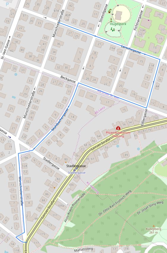
type of environment (land cover data). Figure 2 shows the routes for both regions which
are closest to the best possible solution. Considering the above-mentioned criteria, routes
from A to B achieve the same score as those from B to A. They only differ symmetrically in
slope and frequency of right/left and non-turns. This symmetry causes an equal distance to
the best possible route. Non symmetrical attributes like directed viewsheds would lead to a
difference in score between route A to B and route B to A.
(a) (b)
Figure 2 The closest to average routes for Region 1 (a) and Region 2 (b) considering all criteria
mentioned above (see Sec 3), which were equally weighted.B. Mazurkiewicz, M. Kattenbeck, P. Kiefer, and I. Giannopoulos 8:11
Table 5 Comparison between highest ranked routes and the best possible solution. Land cover
classes are Urban Atlas classes: A (11100), B (11210), C (11220), D (11230), E (12100), F (12220),
G (12230), H (14100) and I (14200). Land cover values do not sum up to 1 due to rounding. If there
are two numbers for a feature this is due to having 2 winners for a region. Why the number of turns
of best possible routes do not sum up to 10 is explained in the discussion.
Avg. # Intersec. # Turns Slope Avg. # Avg. Uniq. Regularity Land Cover %
Name
Options 3 4 5 6 l s r neg none pos of POIs of POIs 3 4 5 6 A B C D E F G H I
Win. Reg 1 3.7 3 7 0 0 4/4 2 4/4 .05/0 .95 .05/0 .2 .2 55.68 16.31 NaN NaN .57 0 0 0 .09 .34 0 0 0
Best Reg 1 3.7 3 7 0 0 4 3 4 .03 .94 .03 .3 .17 51.97 17.24 83.2 69.34 .54 0 0 0 .09 .36 0 .01 0
Win. Reg 2 3.9 3 5 2 0 3/4 3 4/3 .03/.06 .91 .06/.03 0 0 57.75 19.86 72.80 NaN 0 .09 .48 .07 0 .36 0 0 0
Best Reg 2 3.9 3 5 2 0 3 3 3 .08 .84 .08 0 0 58.98 18.30 72.59 148.46 0 .06 .44 .07 0 .36 .01 .03 .01
Table 5 presents numerical results by providing figures for both, the highest ranked routes
(will be referred to as winners) and the best possible solution, i.e., a hypothetical route which
shows closest to average values for all criteria (will be referred to as best). Two aspects are
important to be kept in mind: 1) The best possible solution does not need to be an actually
existing route (see Sec 6); 2) there are two winners per region as each route can be traversed
in both directions.
For both regions, the distribution of scores (i.e., the euclidean distance to the best possible
solution) is similar (see discussion for an explanation of the maxima). The quantiles for the
score in Region 1 are 0%: 0.2250, 25%: 0.5894, 50%: 0.7290, 75%: 0.8569 and 100%: 32.3001.
The score quantiles in Region 2 are 0%: 0.1738, 25%: 0.5198, 50%: 0.6468, 75%: 0.8875,
100%: 5.2246. Regarding the cardinality of DPs, both winners in each region show a perfect
match with best, respectively. With respect to slope, winners 1 are closer to best 1 than
winners 2 are to best 2. It is vice versa regarding POIs, in which case winners 2 match best
2 perfectly (generally speaking, Region 2 is an area which is poor in POIs), whereas winners
1 have, on average, slightly less POIs at a DP than the best possible solution, but their
uniqueness is higher. Looking at the regularity of DPs both routes reflect global averages
very well if and only if they have this kind of n-way intersection6 . Regarding land cover the
differences between winners and best in both regions are minimal7 . Regarding frequency of
right/left and non-turns winners in Region 1 show one continuation less than the winner,
whereas winners in Region 2 show either one left or right more than the best possible route.
In both cases, the frequency of the best possible route is impossible to achieve (see Sec 6
below). Taken together, both winners in each region come close to the best possible route –
which is hypothetical in this case and very unlikely to exist in general but reflects global
averages as good as possible.
6 Discussion
In this work we propose and evaluate a systematic approach for the selection of pedestrian
routes in a street network, with a focus on wayfinding experiments. As described in the
related work section, a proper selection of street routes is crucial for several types of empirical
studies. Such a systematic approach can help select a route based on a multitude of criteria
and, furthermore, reduce the time necessary for manual selection. Moreover, the proposed
approach can be seen as a step towards replicability of research, allowing to select a similar
route at a completely different geographic location by exchanging the best possible solution
6
NaN in a route are not contributing to the euclidean distance.
7
If land cover does not sum up to 1 this is due to rounding.
GIScience 20218:12 Systematic Route Selection
with the target route of another location. The proposed approach was evaluated utilizing
synthetic data serving as a ground truth. The results of this evaluation confirmed the validity
and applicability of our approach. We performed a proof of concept evaluation using real
data, once taken from the city center and once from a residential area in Vienna, Austria.
Two aspects of the results achieved for the real-world data need to be discussed in more
detail: Firstly, the difference in distance between the the upper quartile and the maximum
is very large for Region 1. However, the two routes (out of 62 294) having scores above 32
both have a 6-way intersection – a feature which is very uncommon for Region 1. Obviously,
Region 2 has no large outliers as the maximum euclidean distance is far less than for Region
1. For both regions, however, the distances up to the upper quartile are numerically small;
it is, therefore, a matter of future research whether these differences are meaningful for
wayfinding research and with respect to which criteria this might be the case (see Section 7).
Secondly, the fact that the best possible solutions do not match the predefined number of
DPs by one needs in-depth discussion. All best possible solutions are calculated based on
a z-score, which depends on the population mean and standard deviation. Due to the size
of the population of possible routes, it is very unlikely that mean and standard deviations
both are integers. The number of right, left and non-turns on an actual route (which is
the third factor needed to calculate a z-score), however, must be integers. The figures need
to be rounded (i.e., either floored or ceiled depending on the decimal digits), accordingly.
In addition to that, the means of right and left turns must be symmetric. Hence, the best
possible solution as a hypothetical route can show this anomaly of more/less (±1) DPs than
actually requested, whereas all actual routes in the population always have the predefined
number of decision points (and turns). It is important to note that, although slope is a
symmetric feature as well, its value can be decimal. Moreover, all other criteria are invariant
to the direction of travel on a route. To conclude, our framework supports systematic and
deterministic route selection for experiments considering weighted features provided by the
researcher. Furthermore, exchanging the best possible solution with another target route
(using this route as the average one) allows to find a similar route in a different place of the
world.
The criteria utilized in this work served as an example and can be easily extended or even
replaced by others. Of course, the more criteria used, the longer the route in terms of DPs,
or the larger the search area, the more computation time will be required. In most cases,
however, finding a reasonable route at the city level should be sufficient and this should be
possible in less than one day of computing time as our results were. Our methodological
framework allows to extend the list of criteria taken into account. Several aspects come to
mind: the segment length and orientation might be worthwhile to be taken into account; if
doing so, the number of POIs per segment of a given length may be worthwhile to take into
consideration in order to study on-route landmarks (see [28]). Traffic data, flow of humans
in an area and noise (e.g., stemming from factories) may have an impact on in-situ studies
and might be considered, although it might be very difficult to obtain this type of data on a
large-scale basis. While DPs per se have been extensively considered already, the order of
turns (e.g., llrrslr) and the sequence of intersection types might be included (see e.g., [12]).
One particularly important environmental feature, which is also missing due to unavailability
of large-scale data, is the architectural style/diversity of buildings in a given area.
Computation time and difficulty of validating the results obtained from real data are
the main limitations of this work. Concerning computation time, although this approach
cannot be utilized for real-time purposes, most of the relevant cases for wayfinding will not
be affected by that. Nevertheless, reducing computation time based on existing sub-graphB. Mazurkiewicz, M. Kattenbeck, P. Kiefer, and I. Giannopoulos 8:13
search algorithms is already feasible (see Section 4), although this is out of the scope of
our work. Results for real data are difficult, if not impossible, to validate. Synthetic data
approaches for validation like the one presented above, however, ensure the validity of the
results at least for the cases covered.
7 Conclusion and Outlook
The proposed approach can be considered as a valuable methodological framework, which
can help to make informed decisions concerning route selections. As a consequence, this
framework can partially support the design of experiments and enhance replicability.
The results of the presented approach strongly rely on the availability of appropriate
data sources. The availability of pre-computed data, such as DP type and regularity [10] are
crucial for lowering the required computational costs. As a consequence, we will follow the
path of open data and pre-compute several features that might be relevant for route selection.
Furthermore, we plan to provide an API8 that will ease the access to our framework and
allow to compute a winner route with minimal effort.
Although for most cases only the best result (i.e., the winner route) is relevant, there
might be cases were the comparison between routes is of interest. Therefore, it is reasonable
to study whether the Euclidean distance is actually justifiable by means of empirical results:
The distance metric chosen should reflect empirical results, i.e., if participants are subject to
routes which differ more, less comparable results should occur and vice versa. We are going
to conduct within-group design wayfinding studies on this problem.
References
1 Vanessa Joy A. Anacta, Jia Wang, and Angela Schwering. Routes to remember: Com-
paring verbal instructions and sketch maps. In Joaquín Huerta, Sven Schade, and Carlos
Granell, editors, Connecting a Digital Europe Through Location and Place - International
AGILE’2014 Conference, Castellon, Spain, 13-16 June, 2014, Lecture Notes in Geoinformation
and Cartography, pages 311–322. Springer, 2014. doi:10.1007/978-3-319-03611-3_18.
2 Crystal J. Bae and Daniel R. Montello. Dyadic route planning and navigation in collaborative
wayfinding. In Sabine Timpf, Christoph Schlieder, Markus Kattenbeck, Bernd Ludwig, and
Kathleen Stewart, editors, 14th International Conference on Spatial Information Theory,
COSIT 2019, September 9-13, 2019, Regensburg, Germany, volume 142 of LIPIcs, pages
24:1–24:20. Schloss Dagstuhl - Leibniz-Zentrum für Informatik, 2019. doi:10.4230/LIPIcs.
COSIT.2019.24.
3 Christina Bauer and Bernd Ludwig. Schematic maps and indoor wayfinding. In Sabine Timpf,
Christoph Schlieder, Markus Kattenbeck, Bernd Ludwig, and Kathleen Stewart, editors,
14th International Conference on Spatial Information Theory, COSIT 2019, September 9-13,
2019, Regensburg, Germany, volume 142 of LIPIcs, pages 23:1–23:14. Schloss Dagstuhl -
Leibniz-Zentrum für Informatik, 2019. doi:10.4230/LIPIcs.COSIT.2019.23.
4 Mark de Berg, Otfried Cheong, Marc van Kreveld, and Mark Overmars. Computational
Geometry: Algorithms and Applications. Springer-Verlag TELOS, Santa Clara, CA, USA, 3rd
ed. edition, 2008.
5 Geoff Boeing. Planarity and street network representation in urban form analysis. Environment
and Planning B: Urban Analytics and City Science, 2018. doi:10.1177/2399808318802941.
6 Kenneth Bollen, John T. Cacioppo, Robert M. Kaplan, Jon A. Krosnick, and James L. Olds.
Social, behavioral, and economic sciences perspectives on robust and reliable science. Report
8
Check https://geoinfo.geo.tuwien.ac.at/index.php/resources/ for updates
GIScience 20218:14 Systematic Route Selection
of the Subcommittee on Replicability in Science Advisory Committee to the National Science
Foundation Directorate for Social, Behavioral, and Economic Sciences, 2015. last access on
Mar 5th, 2020. URL: https://www.nsf.gov/sbe/AC_Materials/SBE_Robust_and_Reliable_
Research_Report.pdf.
7 Tad T. Brunyé, Shaina B. Martis, Breanne Hawes, and Holly A. Taylor. Risk-taking during
wayfinding is modulated by external stressors and personality traits. Spatial Cognition &
Computation, 19(4):283–308, 2019.
8 Vincenzo Carletti, Pasquale Foggia, Alessia Saggese, and Mario Vento. Challenging the
time complexity of exact subgraph isomorphism for huge and dense graphs with vf3. IEEE
Transactions on Pattern Analysis and Machine Intelligence, 40:804–818, 2018.
9 Matt Duckham, Stephan Winter, and Michelle Robinson. Including landmarks in routing
instructions. Journal of Location Based Services, 4(1):28–52, 2010.
10 Paolo Fogliaroni, Dominik Bucher, Nikola Jankovic, and Ioannis Giannopoulos. Intersections
of Our World. In Stephan Winter, Amy Griffin, and Monika Sester, editors, 10th International
Conference on Geographic Information Science (GIScience 2018), pages 3:1–3:15, Dagstuhl,
Germany, 2018. Schloss Dagstuhl–Leibniz-Zentrum fuer Informatik.
11 Ioannis Giannopoulos, David Jonietz, Martin Raubal, Georgios Sarlas, and Lisa Stähli. Timing
of pedestrian navigation instructions. In Eliseo Clementini, Maureen Donnelly, May Yuan,
Christian Kray, Paolo Fogliaroni, and Andrea Ballatore, editors, 13th International Conference
on Spatial Information Theory, COSIT 2017, September 4-8, 2017, L’Aquila, Italy, volume 86
of LIPIcs, pages 16:1–16:13. Schloss Dagstuhl - Leibniz-Zentrum für Informatik, 2017. doi:
10.4230/LIPIcs.COSIT.2017.16.
12 Ioannis Giannopoulos, Peter Kiefer, and Martin Raubal. GazeNav: Gaze-Based Pedestrian Nav-
igation. In Proceedings of the 17th International Conference on Human-Computer Interaction
with Mobile Devices & Services, MobileHCI ’15, pages 337–346. ACM, 2015.
13 Charalampos Gkonos, Ioannis Giannopoulos, and Martin Raubal. Maps, vibration or gaze?
Comparison of novel navigation assistance in indoor and outdoor environments. Journal of
Location Based Services, 11(1):29–49, 2017.
14 Jana Götze and Johan Boye. "turn left" versus "walk towards the café": When relative directions
work better than landmarks. In Fernando Bação, Maribel Yasmina Santos, and Marco Painho,
editors, AGILE 2015 - Geographic Information Science as an Enabler of Smarter Cities
and Communities, Lisboa, Portugal, 9-12 June 2015, Lecture Notes in Geoinformation and
Cartography, pages 253–267. Springer, 2015. doi:10.1007/978-3-319-16787-9_15.
15 Jiawei Han, Micheline Kamber, and Jian Pei. 2 - getting to know your data. In Jiawei
Han, Micheline Kamber, and Jian Pei, editors, Data Mining (Third Edition), The Morgan
Kaufmann Series in Data Management Systems, pages 39–82. Morgan Kaufmann, Boston,
third edition edition, 2012.
16 Gengen He, Toru Ishikawa, and Makoto Takemiya. Collaborative navigation in an unfamiliar
environment with people having different spatial aptitudes. Spatial Cognition & Computation,
15(4):285–307, 2015.
17 Toru Ishikawa and Uiko Nakamura. Landmark selection in the environment: Relationships
with object characteristics and sense of direction. Spatial Cognition & Computation, 12(1):1–22,
2012.
18 Markus Kattenbeck. How subdimensions of salience influence each other. comparing models
based on empirical data. In Eliseo Clementini, Maureen Donnelly, May Yuan, Christian
Kray, Paolo Fogliaroni, and Andrea Ballatore, editors, 13th International Conference on
Spatial Information Theory, COSIT 2017, September 4-8, 2017, L’Aquila, Italy, volume 86
of LIPIcs, pages 10:1–10:13. Schloss Dagstuhl - Leibniz-Zentrum für Informatik, 2017. doi:
10.4230/LIPIcs.COSIT.2017.10.
19 Markus Kattenbeck, Eva Nuhn, and Sabine Timpf. Is salience robust? A heterogeneity
analysis of survey ratings. In 10th International Conference on Geographic Information
Science, GIScience 2018, August 28-31, 2018, Melbourne, Australia, volume 114 of LIPIcs,B. Mazurkiewicz, M. Kattenbeck, P. Kiefer, and I. Giannopoulos 8:15
pages 7:1–7:16. Schloss Dagstuhl - Leibniz-Zentrum für Informatik, 2018. doi:10.4230/LIPIcs.
GISCIENCE.2018.7.
20 Peter Kedron, Amy E. Frazier, Andrew B. Trgovac, Trisalyn Nelson, and A. Stewart Foth-
eringham. Reproducibility and replicability in geographical analysis. Geographical Analysis,
NA(NA):NA, 2020. doi:10.1111/gean.12221.
21 Peter Kiefer, Ioannis Giannopoulos, and Martin Raubal. Where am I? Investigating map match-
ing during self-localization with mobile eye tracking in an urban environment. Transactions in
GIS, 18(5):660–686, 2014.
22 Vasiliki Kondyli, Carl P. L. Schultz, and Mehul Bhatt. Evidence-based parametric design: Com-
putationally generated spatial morphologies satisfying behavioural-based design constraints. In
Eliseo Clementini, Maureen Donnelly, May Yuan, Christian Kray, Paolo Fogliaroni, and Andrea
Ballatore, editors, 13th International Conference on Spatial Information Theory, COSIT 2017,
September 4-8, 2017, L’Aquila, Italy, volume 86 of LIPIcs, pages 11:1–11:14. Schloss Dagstuhl
- Leibniz-Zentrum für Informatik, 2017. doi:10.4230/LIPIcs.COSIT.2017.11.
23 Markus Konkol, Christian Kray, and Morin Ostkamp. Follow the signs - countering disen-
gagement from the real world during city exploration. In Arnold K. Bregt, Tapani Sarjakoski,
Ron van Lammeren, and Frans Rip, editors, Societal Geo-innovation - Selected Papers of
the 20th AGILE Conference on Geographic Information Science, Wageningen, The Nether-
lands, 9-12 May 2017, Lecture Notes in Geoinformation and Cartography, pages 93–109, 2017.
doi:10.1007/978-3-319-56759-4_6.
24 Markus Konkol, Christian Kray, and Max Pfeiffer. Computational reproducibility in
geoscientific papers: Insights from a series of studies with geoscientists and a reproduction
study. International Journal of Geographical Information Science, 33(2):408–429, 2019.
25 Hengshan Li and Nicholas A. Giudice. Assessment of between-floor structural and topological
properties on cognitive map development in multilevel built environments. Spatial Cognition
& Computation, 18(3):138–172, 2018.
26 Hua Liao, Weihua Dong, Haosheng Huang, Georg Gartner, and Huiping Liu. Inferring
user tasks in pedestrian navigation from eye movement data in real-world environments.
International Journal of Geographical Information Science, 33(4):739–763, 2019.
27 Lynn S. Liben, Lauren J. Myers, and Adam E. Christensen. Identifying locations and
directions on field and representational mapping tasks: Predictors of success. Spatial Cognition
& Computation, 10(2-3):105–134, 2010.
28 K L Lovelace, M Hegarty, and D R Montello. Elements of good route directions in familiar
and unfamiliar environments. In Freksa, C. and Mark, D. M., editor, Spatial Information
Theory: Cognitive and Computational Foundations of Geographic Information Science, Lecture
Notes in Computer Science, pages 65–82, 1999.
29 William A. Mackaness, Phil J. Bartie, and Candela Sanchez-Rodilla Espeso. Understanding
information requirements in "text only" pedestrian wayfinding systems. In Geographic Inform-
ation Science - 8th International Conference, GIScience 2014, Vienna, Austria, September
24-26, 2014. Proceedings, volume 8728 of Lecture Notes in Computer Science, pages 235–252.
Springer, 2014. doi:10.1007/978-3-319-11593-1_16.
30 N. Magdy, M. A. Sakr, T. Mostafa, and K. El-Bahnasy. Review on trajectory similarity
measures. In 2015 IEEE Seventh International Conference on Intelligent Computing and
Information Systems (ICICIS), pages 613–619, December 2015.
31 Stefan Münzer and Christoph Stahl. Learning routes from visualizations for indoor wayfinding:
Presentation modes and individual differences. Spatial Cognition & Computation, 11(4):281–
312, 2011.
32 Daniel Nüst, Carlos Granell, Barbara Hofer, Markus Konkol, Frank O. Ostermann, Rusne
Sileryte, and Valentina Cerutti. Reproducible research and GIScience: an evaluation using
AGILE conference papers. PeerJ, 6:e5072, 2018.
33 Christina Ohm, Manuel Müller, and Bernd Ludwig. Evaluating indoor pedestrian navigation
interfaces using mobile eye tracking. Spatial Cognition & Computation, 17(1-2):89–120, 2017.
GIScience 20218:16 Systematic Route Selection
34 Open Science Collaboration. Reproducibility Project: Psychology, 2015.
35 Frank O. Ostermann and Carlos Granell. Advancing science with vgi: Reproducibility and
replicability of recent studies using vgi. Transactions in GIS, 21(2):224–237, 2017.
36 Marianna Pagkratidou, Alexia Galati, and Marios Avraamides. Do environmental characterist-
ics predict spatial memory about unfamiliar environments? Spatial Cognition & Computation,
20(1):1–32, 2020.
37 Martin Perebner, Haosheng Huang, and Georg Gartner. Applying user-centred design for
smartwatch-based pedestrian navigation system. Journal of Location Based Services, 13(3):213–
237, 2019.
38 Karl Rehrl, Elisabeth Häusler, and Sven Leitinger. Comparing the effectiveness of gps-enhanced
voice guidance for pedestrians with metric- and landmark-based instruction sets. In Geographic
Information Science, 6th International Conference, GIScience 2010, Zurich, Switzerland,
September 14-17, 2010. Proceedings, volume 6292 of Lecture Notes in Computer Science, pages
189–203. Springer, 2010. doi:10.1007/978-3-642-15300-6_14.
39 Karl Rehrl, Elisabeth Häusler, Sven Leitinger, and Daniel Bell. Pedestrian navigation with
augmented reality, voice and digital map: final results from an in situ field study assessing
performance and user experience. Journal of Location Based Services, 8(2):75–96, 2014.
40 Karl Rehrl, Sven Leitinger, Georg Gartner, and Felix Ortag. An analysis of direction and
motion concepts in verbal descriptions of route choices. In Kathleen Stewart Hornsby, Chris-
tophe Claramunt, Michel Denis, and Gérard Ligozat, editors, Spatial Information Theory,
9th International Conference, COSIT 2009, Aber Wrac’h, France, September 21-25, 2009,
Proceedings, volume 5756 of Lecture Notes in Computer Science, pages 471–488. Springer,
2009. doi:10.1007/978-3-642-03832-7_29.
41 Adam Rousell and Alexander Zipf. Towards a landmark-based pedestrian navigation service
using osm data. ISPRS International Journal of Geo-Information, 6(3):64, 2017.
42 Wiebke Schick, Marc Halfmann, Gregor Hardiess, Friedrich Hamm, and Hanspeter A. Mallot.
Language cues in the formation of hierarchical representations of space. Spatial Cognition &
Computation, 19(3):252–281, 2019.
43 Helmut Schrom-Feiertag, Volker Settgast, and Stefan Seer. Evaluation of indoor guidance sys-
tems using eye tracking in an immersive virtual environment. Spatial Cognition & Computation,
17(1-2):163–183, 2017.
44 S. Schwarzkopf, S. J. Büchner, C. Hölscher, and L. Konieczny. Perspective tracking in the
real world: Gaze angle analysis in a collaborative wayfinding task. Spatial Cognition &
Computation, 17(1-2):143–162, 2017.
45 Angela Schwering, Jakub Krukar, Rui Li, Vanessa Joy Anacta, and Stefan Fuest. Wayfinding
through orientation. Spatial Cognition & Computation, 17(4):273–303, 2017.
46 Makoto Takemiya and Toru Ishikawa. I can tell by the way you use your walk: Real-
time classification of wayfinding performance. In Max J. Egenhofer, Nicholas A. Giudice,
Reinhard Moratz, and Michael F. Worboys, editors, Spatial Information Theory - 10th
International Conference, COSIT 2011, Belfast, ME, USA, September 12-16, 2011. Proceedings,
volume 6899 of Lecture Notes in Computer Science, pages 90–109. Springer, 2011. doi:
10.1007/978-3-642-23196-4_6.
47 Makoto Takemiya and Toru Ishikawa. Strategy-based dynamic real-time route prediction. In
Thora Tenbrink, John G. Stell, Antony Galton, and Zena Wood, editors, Spatial Information
Theory - 11th International Conference, COSIT 2013, Scarborough, UK, September 2-6, 2013.
Proceedings, volume 8116 of Lecture Notes in Computer Science, pages 149–168. Springer,
2013. doi:10.1007/978-3-319-01790-7_9.
48 Lin Wang, Weimin Mou, and Xianghong Sun. Development of landmark knowledge at decision
points. Spatial Cognition & Computation, 14(1):1–17, 2014.
49 Flora Wenczel, Lisa Hepperle, and Rul von Stülpnagel. Gaze behavior during incidental
and intentional navigation in an outdoor environment. Spatial Cognition & Computation,
17(1-2):121–142, 2017.You can also read