An open tool for creating battery-electric vehicle time series from empirical data - emobpy
←
→
Page content transcription
If your browser does not render page correctly, please read the page content below
An open tool for creating battery-electric vehicle time series from
                                                                                       empirical data - emobpy

                                                  Carlos Gaete-Morales1 , Hendrik Kramer2 , Wolf-Peter Schill3 , and Alexander Zerrahn4
arXiv:2005.02765v2 [physics.soc-ph] 12 Feb 2021

                                                   1
                                                       German Institute for Economic Research (DIW Berlin), Mohrenstr. 58, D-10117 Berlin, Germany,
                                                                                                     cgaete@diw.de.
                                                           2
                                                               Technische Universität Berlin, D-10623 Berlin, Germany, hendrik.kramer@uni-due.de.
                                                   3
                                                       German Institute for Economic Research (DIW Berlin), Mohrenstr. 58, D-10117 Berlin, Germany,
                                                                                                    wschill@diw.de.
                                                   4
                                                       German Institute for Economic Research (DIW Berlin), Mohrenstr. 58, D-10117 Berlin, Germany,
                                                                                                    azerrahn@diw.de.

                                                                                                  February 15, 2021

                                                                                                         Abstract
                                                         There is substantial research interest in how future fleets of battery-electric vehicles will interact with
                                                         the power sector. To this end, various types of energy models depend on meaningful input parameters,
                                                         in particular time series of vehicle mobility, driving electricity consumption, grid availability, or grid
                                                         electricity demand. As the availability of such data is highly limited, we introduce the open-source
                                                         tool emobpy. Based on mobility statistics, physical properties of vehicles, and other customizable as-
                                                         sumptions, it derives time series data that can readily be used in a wide range of model applications.
                                                         For an illustration, we create and characterize 200 battery-electric vehicle profiles for Germany. De-
                                                         pending on the hour of the day, a fleet of one million vehicles has a median grid availability between
                                                         5 and 7 gigawatts, as vehicles are parking most of the time. Four exemplary grid electricity demand
                                                         time series illustrate the smoothing effect of balanced charging strategies.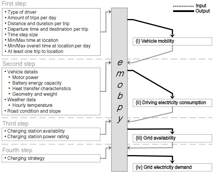
1   INTRODUCTION

1     Introduction
We introduce emobpy. It is an open-source python-based tool that creates profiles of battery-electric
vehicles (BEV), based on empirical mobility statistics and customizable assumptions. We additionally
provide a first application of the tool and create vehicle profiles based on representative German mobility
data. An emobpy profile consists of four time series: (i) vehicle mobility containing the vehicle’s location
and distance travelled, (ii) driving electricity consumption, specifying how much electricity is taken from
the battery for driving; (iii) BEV grid availability, providing information whether and with which power
rating a BEV is connected to the electricity grid at a certain point in time; and (iv) BEV grid electric-
ity demand, specifying the actual charging electricity drawn from the grid, based on different charging
strategies.

Such profiles are core input data for a wide range of model applications in energy, environmental, and
economic studies on BEV. Technology developments as well as energy and climate policy measures drive
the deployment of BEV in many countries [1]. Growing BEV fleets can have substantial impacts on the
power sector. They increase the electric load, but may also provide temporal flexibility for integrating
variable renewable energy sources and contribute to decarbonizing transportation [2]. Many model-based
analyses investigate potential power sector interactions of future BEV fleets [3–6] and thus depend on a
meaningful representation of electric vehicles’ mobility patterns.

Yet such data are often not publicly available. In general, empirical data are scarce because BEV fleets
are still small in most countries. And if respective time series are available, they are often specific to the
conditions in which the data was collected and subject to data protection provisions. Past approaches
make either stylized coarse assumptions [7], derive data from mobility statistics, but lack documentation,
transparency or reproducibility [8–14], or are idiosyncratic with respect to geographic characteristics or
assumed driver behavior [11, 15, 16].

                                                      1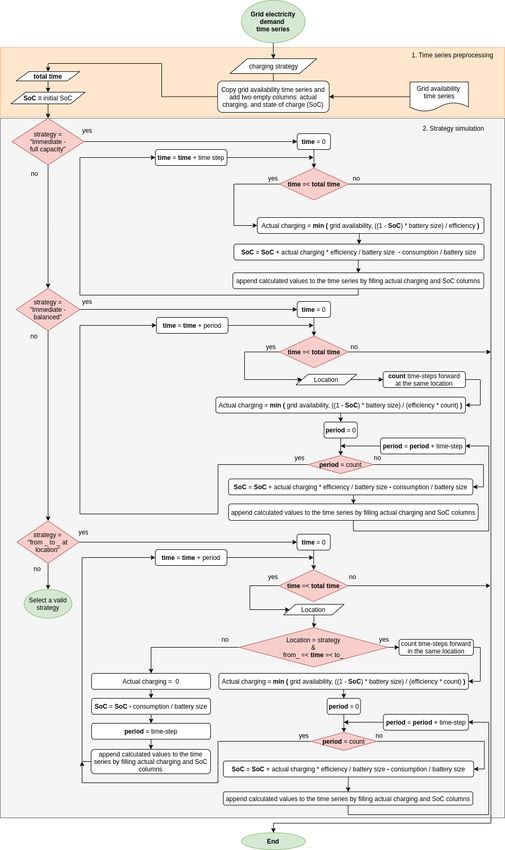
1   INTRODUCTION

Figure 1: Inputs and outputs for emobpy and sequence of generating four types of time series. The boxes
on the left-hand side show customizable input assumptions, the boxes on the right-hand side indicate the
four types of time series.

Following [3], we argue that new models are needed to derive relevant time series in a transparent and
flexible way. As a first step in this direction, the tools Vencopy [17] and RAMP-mobility [18] recently
emerged. To further fill this gap, we developed emobpy. Our tool takes empirical mobility statistics,
physical properties of vehicles, and customizable assumptions as inputs and delivers BEV profiles as
output. Figure 1 gives a stylized account. We first discuss the outputs, then the required inputs.

Four output time series constitute one BEV profile. These profiles have a customizable length and
resolution. A handy format for many applications is all hours of one year. But also other formats are
possible by discretion of the researcher. Likewise, the researcher can choose how many profiles she wants
to create.

The time series of vehicle mobility (i) contains the location of the vehicle at each time step and the
time steps during which the vehicle is driving with information of the distance traveled. The driving
electricity consumption time series (ii) provides information on how much electricity the vehicle consumes
for driving in each time step. The time series of (iii) grid availability provides information whether a
vehicle is connected to the electricity grid in a time step and if so, with what power rating for charging or
discharging. The time series of grid electricity demand (iv) provides information on how much electricity
a vehicle demands from the electricity grid in a time step. Time series (i), (ii) and (iii) are core inputs for
models that endogenously determine the timing of charging (and, potentially, discharging to the grid);

                                                      2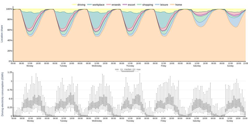
2   RESULTS

the time series (iv) are core inputs for models that do not endogenously determine the grid interactions
of BEV, but use exogenous input data for this.

The required input data for the time series of vehicle mobility (i) are the relative frequencies of different
driver types, e.g., commuters, of the number of trips per day, of the destination, distance and duration
of trips, and of the departure hours. Such information can often be derived from national mobility
statistics. If required or desired, a researcher can also make up own assumptions or resort to the pre-set
values from German mobility statistics. emobpy makes sure that the resulting time series are feasible and
consistent. To this end, a minimum and maximum number of hours at specific locations can specified,
and it is assumed that the last trip of a day heads home. With a Monte Carlo approach, emobpy ensures
variability across profiles.

Based on the vehicle mobility time series, the driving electricity consumption (ii) time series is derived.
This requires further input data, such as information on nominal motor power, curb weight, drag coef-
ficient, and dimensions, which the tool includes for several current BEV models. Ambient temperature
is also a significant parameter that affects the consumption of BEV [8, 19]. For that reason, emobpy is
endowed with a database of hourly temperature for European countries with a registry of the last 17
years. Additionally, the vehicle cabin insulation characteristics are required; this data is not widely avail-
able and thus assumed independently of the BEV models database. Driving cycles are also important
input parameters that are used to simulate every individual trip. The model includes two driving cycles,
Worldwide Harmonized Light Vehicles Test Cycle (WLTC) and Environmental Protection Agency (EPA).
This input data is already provided within the tool, and the user can select a particular BEV model,
country weather and driving cycle. Additionally, emobpy also allows providing user-defined custom data.

The required input data for the grid availability time series (iii) is the driving electricity consumption
time series (ii). Further, data or assumptions on the power rating of charging stations at different generic
locations as well as their availability probabilities are needed. Variability across profiles is, again, intro-
duced through a Monte Carlo approach, while emobpy makes sure that the time series (iii) is consistent
within each profile .

The required input data for the grid electricity demand time series (iv) includes the created time series on
driving electricity consumption (ii) and grid availability (iii). Additionally, users can choose a charging
strategy, such as immediate full charging or night-time charging, or make customary assumptions.

2     Results
2.1    Application to Germany: parameterization and setup
For a first application of emobpy, we draw on the comprehensive German mobility survey Mobilität in
Deutschland [Mobility in Germany, 20]. The survey features mobility data relating to different types of
households, vehicles, individuals, and trips. In this application, we make three general assumptions: first,
we assume that individuals with access to a vehicle carry out all their trips with the same vehicle; second,

                                                      3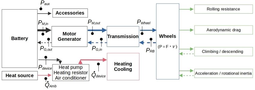
2.1   Application to Germany: parameterization and setup                                    2   RESULTS

we assume that future BEV drivers have similar mobility patterns as current conventional drivers covered
by the underlying mobility statistics; and third, for simplicity and tractability, we assume that there are
only four BEV models: Hyundai Kona, Renault Zoe, Tesla Model 3 and Volkswagen ID.3. These models
had the largest market shares in Germany by the time of writing. Again, all of these pre-set assumptions
can easily be modified in emobpy.

We generate 50 profiles for each BEV model, i.e., 200 BEV profiles overall, each consisting of four time
series. We focus on two types of drivers: commuters (62% of all drivers) and non-commuters (38% of
all drivers). For commuters, we further differentiate between full-time and part-time employees, with a
split of 78 to 22% [21]. We exclude commuting students, apprentices, and trainees, who represent only
a small share of all commuters in the initial dataset. The amount of trips per day varies between 0 - 5
with different probabilities for weekdays and weekend days (Table 1).

  Table 1: Probability distributions (given in %) for the amount of trips per day by days of the week

                   Number of trips         Working days              Weekend days
                           0                    35.4                      50.7
                           1                     0.0                       0.0
                           2                    29.9                      27.5
                           3                     8.3                       4.4
                           4                    12.5                      10.2
                           5                    13.9                       7.2
                  Note: Data adapted from [20]. Commuters have the same distribution of
                  daily trips as non-commuters. Data correspond to the group of respon-
                  dents that have a yearly mileage in the range of 10, 000-15, 000 km.

The trip distance and duration follows a probability distribution derived from the input data (Table 2).
As the underlying mobility statistics features a category that includes any trips with more than 100 km
distance and more than 60 minutes duration, we cap the maximum distance travelled per trip at 400 km
and the trip duration at 185 minutes. We also ensure that the average velocity resulting from every
possible combination of distance and duration cannot exceed 130 km/h.

The probability of departure times is specific to the trip destination, type of driver, and day of the week
(Table 3). It is distributed according to the underlying mobility statistics. Following the input data,
we consider six trip destinations: workplace, shopping, errands, escort, leisure, and home. An example
for errands is a visit to the doctor or to the authorities. In the case of escort destinations, the driver
transports other persons, for example children. A set of rules is implemented in this case study to select
only consistent day trips. The rules are applied depend on day of the week and the type of driver (Table 5
in the Methods section).

Table 4 contains information on the four BEV models used for this case study. Most of the parameters

                                                       4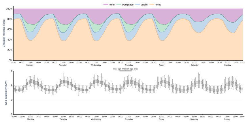
2.1   Application to Germany: parameterization and setup                                                                    2   RESULTS

Table 2: Joint probability distributions (given in %) for the distance travelled by trip and trip duration.

                                                              Trip duration (minutes)
            Distance           10          10 - 15         15 - 20      20 - 30           30 - 45           45 - 60   60 - 185
               1 km            2.9           0.3              0            0                    0              0         0
             1 - 2 km          3.5           4.8             0.8           0                    0              0         0
             2 - 5 km          8.4          10.2             5.7           0                   1.2            0.4        0
            5 - 10 km          1.3          12.2            14.4           0                   2.4            0.6       0.7
           10 - 20 km           0           0.9             6.3            0                   4.7            1.3       0.5
           20 - 50 km           0             0               0            0                   8.6            2.1       1.6
           50 - 100 km          0             0               0            0                    0             0.6       2.1
          100 - 400 km          0             0               0            0                    0              0        1.5
         Note: Data adapted from [20]. Numbers rounded to one decimal. Data correspond to the group
         of respondents that have a yearly mileage in the range of 10, 000-15, 000 km. All values add up
         to 100%.

Table 3: Joint probability distributions (given in %) for trip destinations and departure times, differen-
tiated for commuters and non-commuters and days of the week

                      Work-          Shopping          Errands                  Escort                  Leisure             Home
                      place
       Commuter        yes       yes        no       yes        no        yes            no          yes       no     yes          no

       Departure                                                     Working days

      05:00-08:00      11.1      0.5       0.7       0.5        0.7       1.1            0.7         0.5       0.7    0.8         0.7
      08:00-10:00       3.1      1.8       4.5       1.4        4.1       0.8            0.9         1.4       3.2    1.8        3.6
      10:00-13:00       1.3      2.7       6.7       2.3        5.4       0.7            1.3         3.2       4.7    5.5        11.7
      13:00-16:00       1.1      2.5       3.7       2.2        4.0       1.8            1.5         3.8       5.9    8.9        8.2
      16:00-19:00       0.3      3.0       1.9       2.2        2.2       1.4            1.0         4.9       4.5    14.0        9.3
      19:00-22:00       0.3      0.4       0.1       0.6        0.4       0.4            0.3         2.4       1.5    6.1        4.0
      22:00-05:00       0.6      0.0       0.0       0.1        0.1       0.1            0.1         0.4       0.2    2.4        1.3

                                                                       Saturday

      05:00-08:00      0.9       1.2       1.2       0.3        0.3       0.2            0.2         0.8       0.8    0.8          0.8
      08:00-10:00      0.5       4.8       4.9       1.9        2.0       0.7            0.7         2.7       2.8    3.0          3.1
      10:00-13:00      0.4       7.1       7.3       3.5        3.6       1.4            1.5         5.2       5.4    9.1          9.3
      13:00-16:00      0.2       3.4       3.5       2.5        2.6       1.2            1.2         7.0       7.1    7.6          7.8
      16:00-19:00      0.1       2.3       2.4       1.7        1.7       1.1            1.1         6.0       6.1    9.5          9.7
      19:00-22:00      0.1       0.4       0.4       0.5        0.5       0.4            0.4         2.5       2.6    4.9          5.0
      22:00-05:00      0.2       0.0       0.0       0.1        0.1       0.2            0.2         0.8       0.8    3.0          3.1

                                                                       Sunday

      05:00-08:00      0.8       0.3       0.3       0.2        0.2       0.1            0.1          0.8       0.8   0.4        0.4
      08:00-10:00      0.4       1.5       1.5       1.4        1.5       0.6            0.6          4.8       4.9   2.0        2.1
      10:00-13:00      0.3       0.7       0.7       2.8        2.8       1.3            1.3         11.7      11.9   7.2        7.4
      13:00-16:00      0.3       0.5       0.5       2.6        2.6       1.4            1.4         13.7      14.0   8.8        9.0
      16:00-19:00      0.2       0.2       0.2       1.8        1.9       1.0            1.0          6.8       7.0   13.3       13.6
      19:00-22:00      0.2       0.1       0.1       0.5        0.5       0.4            0.5          2.0       2.1   6.4        6.6
      22:00-05:00      0.1       0.0       0.0       0.1        0.1       0.1            0.1          0.4       0.4   2.0        2.1
      Note: Data adapted from [20]. Numbers rounded to one decimal.

serve to calculate driving electricity consumption, with the exception of nominal battery capacity that
is used to generate the grid availability time series (iii)and grid demand time series (iv). Many other
parameters are also provided by emobpy to calculate the driving electricity consumption, such as efficien-
cies, auxiliary power and heat transfer data, as shown in Tables 6 and 7 in the Methods section. These
are default values in the tool; however, they can be modified if desired by the user.

We model time steps of 15 minutes. In each time step, a vehicle is either driving in case a trip takes place,

                                                                   5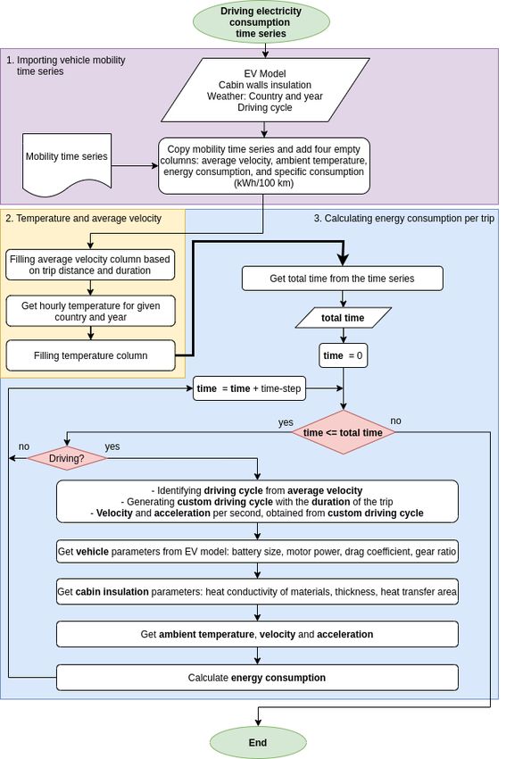
2.1     Application to Germany: parameterization and setup                                  2   RESULTS

                    Table 4: BEV models’ parameters derived from manufacturer data [22]

                                            BEV models
        Parameter     Unit    Model 3     ID.3     Kona       Zoe                Description
                              (Tesla)    (VW)     (Hyundai) (Renault)
         Nmotor       kW         358       93       150         65      Nominal motor power
         Nbattery    kWh        79.5      45.0      64.0       45.6     Nominal battery capacity
           mc         kg        1860      1600      1685       1480     Curb weight
            Cd         -        0.23      0.27      0.29       0.29     Drag coefficient
            h          m        1.44      1.55      1.57       1.56     Height
            w          m        1.85      1.81      1.80       1.73     Width
          rgear        -         9.0      10.0       8.0        9.3     Gear ratio
          P MR       W/kg        192       58        89         44      Power to mass ratio

or is in one of the locations workplace, shopping, and so on. Depending on the vehicle location, a charging
station to connect the vehicle to the grid may be available with a location-specific power rating. For this
application, we assume four generic types of charging stations with different probability distributions for
each vehicle location. The charging stations are at home, in the public area, or at the workplace, or none
is available. Respective power ratings are 3.6, 22, 11, and 0 kW, based on [23]. The tool also considers
fast charging; this feature is available for long-distance trips that are larger than the vehicle maximum
range. The charging capacities selected for this application are 75 and 150 kW. This can be interpreted
as the vehicle making a short stop during a longer trip. Charging efficiency is set to 90% (cp. [6, 9, 15,
24]).

When at home, 81% of all drivers park their vehicles in a carport or garage and 19% on public streets
according to [20]. For the group of vehicle profiles that have a carport at home, we assume a 100%
charging availability. For those without a private charging station, we set a probability of 50% to find a
public charging station and 50% of finding none. For commuters, we consider three charging groups with
different grid connection opportunities during work hours: charging at the workplace, charging in the
public area, or none. When commuters park their BEV at the workplace, we assume that 50% of them
can charge their vehicles there, with a 100% probability of finding a charging station; 25% of commuters
charge in a public area, with a 50% probability of finding a charging station; and the remaining 25% of
commuters are assumed to have a 100% probability of not having a charging station available during work
hours (none). For the vehicle locations shopping, errands, escort, and leisure, we assume a probability
of 50% to find a public charging station and 50% to find none. When driving, grid connection is not
available, with the exception of fast-charging for very long trips.

To derive time series of BEV grid electricity demand, we apply four exemplary charging strategies. Note
that these charging strategies do not take into account any power sector or electricity market price
information:

      • immediate - full capacity: BEV charge their batteries at full power rating as soon as they arrive
         at charging stations. Charging stops when the battery is full, or when the next trip starts. This

                                                      6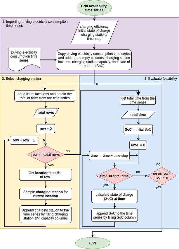
2.2    Vehicle mobility                                                                        2   RESULTS

        mimics a setting where drivers have no incentives and/or no technical possibility to charge their
        vehicle batteries in a more balanced way, which is likely to be sub-optimal with respect to the
        electricity market or network situation.

      • immediate - balanced : BEV start charging their batteries as soon as they arrive at charging stations,
        however with constant power rating (usually below the power rating of the charging station), such
        that a 100% state of charge is reached just before starting the next trip, assuming perfect foresight
        of the next departure time. This approximates a smoother and potentially more system-oriented
        charging behaviour.

      • at home - balanced : similar to the previous charging strategy, but BEV only charge at home, even
        when additional charging options are available at other locations. This reflects a preference or
        economic incentive for home charging.

      • at home night-time - balanced : similar to the previous charging strategy, but with charging time
        restricted to the time window between 23:00 and 8:00. This mimics the effect of potential tariff
        incentives for night-time (off-peak) charging.
2.2      Vehicle mobility
Figure 2 summarizes all 200 simulated vehicle mobility time series. For each hour, vehicle locations are
averaged over all profiles and weeks of the year. Hourly driving electricity consumption is summarized in
box plots, rendering the dispersion over the simulated profiles through the weeks of the year. All numbers
are linearly scaled up to represent one million BEV, so the setting may be interpreted as a near-term
future scenario.

Most of the time, vehicles are parking (top panel). At night, between 23:00 and 5:00, more than 96% of the
fleet are, on average, at home. During daytime, still the majority of vehicles are at home, but also a large
proportion of vehicles is at the workplace, peaking at 32% at 11:00 on working days. During weekends,
more vehicles stay at home, and the shares of shopping, errands, escort, and leisure increase. Commuters
have a positive but very small probability of going to the workplace on weekends (Tables 3 and 5), so it
is hardy visible in Figure 2. Every day between 6:00 and 22:00, at least 3% of the fleet are driving, with
a peak between around 15:00 and 17:00 with about 9% of the fleet driving.

To validate emobpy results, we compare the cumulative distributions of trips and mileage to the underlying
German mobility statistics [20]. For the two metrics, the cumulative distributions follow a similar pattern
(Figure 3). Both our emobpy application and the official German statistics indicate that about 90% of
all trips have a distance travelled of 50 km or below. The cumulative mileage – the overall distance
travelled by all vehicles in a year – also has a similar shape in emobpy and in the official statistics up
to 40 km. The Figure also allows inferring that long-distance trips above 100 km represent 25% of the
yearly mileage, while those trips only account for 3% of all trips [20]

                                                         7
2.3 Driving electricity consumption 2 RESULTS
Figure 2: Simulated time series of vehicle locations (top panel) and driving electricity consumption
(bottom panel) of one million BEV, given as averages and box plots for each hour of the week.
Figure 3: Comparison of cumulative shares of trips and mileage per distance travelled. “Germany”
represents German mobility statistics [20], which reports these aggregate shares up to a distance of 100 km.
2.3 Driving electricity consumption
The overall hourly driving electricity consumption of one million BEV (Figure 2, bottom panel) peaks
between 15:00 and 17:00 on working days with an annual median around 450 MWh, and an absolute
maximum at 19:00 of 1250 MWh. During the weekend, overall consumption is lower and with less
distinctive evening peaks.
The average specific consumption for all trips over the 200 profiles and four models is 22.2 kWh/100 km.
The median specific consumption values for the different BEV types Model 3, Kona, ID.3 and Zoe are
22.7, 17.9, 15.7, and 14.5 kWh/100 km, respectively (Figure 4). The ambient temperature variation has
a clear impact on the specific consumption. On average, specific consumption is lowest in summer with
20.7 kWh/100 km, and highest in winter with 23.6 kWh/100 km.
82.4 Grid availability 2 RESULTS
Figure 4: Specific consumption of four selected BEV models throughout a year. The values are calculated
as the medians of all trips taken for every three days.
2.4 Grid availability
The cumulative simulated grid availability time series is shown in Figure 5. On working days, the time
series on the types of charging stations has a recurring pattern (top panel) that corresponds to the
pattern of vehicle locations. The share of vehicles with a charging station available reaches a 90% peak
between 3:00 and 5:00 at night. Here, around 80% of vehicles are connected at home and 10% on a public
street. Between 11:00 and 12:00, average grid availability is at a minimum level of 70%. During daytime,
a relevant proportion of available charging stations is at the workplace. On weekends, the charging station
time series is less peaky, with higher proportions at home and on public streets during daytime.
The grid-connected power rating is lowest between 19:00 and 8:00, with a median between 5.0 and 5.6 GW
for a fleet of one million BEV (bottom panel). This is due to the high share of home charging stations
with a low power rating of 3.6 kW. During daytime, the median grid-connected power rating is greater
than 7 GW because charging stations available either at the workplace or in public areas have a power
rating of 11 and 22 kW, respectively.
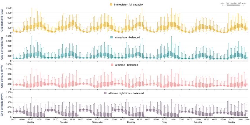
2.5 Grid electricity demand
The grid electricity demand time series for the four exemplary charging strategies are summarized in
Figure 6. The immediate - full capacity charging strategy leads to a volatile cumulative BEV grid
electricity demand both over the week and over the year, with a pronounced diurnal pattern. A distinctive
peak of hourly electricity demand from the grid, with median values around 460 MWh for a fleet of one
million BEV, occurs on working day afternoons between 17:00 and 20:00, when many vehicles arrive
at home and charge immediately at full power rating. As the entire BEV fleet is assumed to charge
similarly in this scenario, such a charging strategy would substantially add to the evening peak of electric
93 DISCUSSION
Figure 5: Simulated time series summarized for different types of charging stations (top panel) and grid-
connected power rating (bottom panel) of one million BEV, given as averages and box plots for each hour
of the week.
load. It could thus have substantial repercussions on the power sector and other electricity consumers.
Load peaks could increase even further if higher power rating for charging at home beyond 22 kW was
considered.
The immediate - balanced and at home - balanced charging strategies have smoother temporal grid
electricity demand patterns with lower peaks, because vehicles do not get charged at full power rating
once they reach a charging station. Both the variance of medians and (interquartile) ranges are lower.
Likewise, the median hourly consumption of the one million BEV fleet rarely exceeds 400 MWh for
immediate - balanced, and 300 MWh for at home - balanced. During weekdays, fluctuations are more
pronounced for at home - balanced, as most vehicles are at home every night. Compared to immediate -
full capacity, such smoother charging may be more compatible with the power sector.
The at home night-time - balanced charging strategy shows a distinct load peak at working day nights,
with median hourly grid electricity demand of one million BEV around 420 MWh. Between Friday evening
and Monday morning, median demand at night-time is lower than 300 MWh because the vehicles are less
used on weekends than on working days. Accordingly, any regulatory measures that shift BEV charging
to night-time periods would lead to substantially less smooth patterns compared to all-day charging. Yet
the power sector implications of these charging strategies are less clear and should be investigated in
detail with dedicated energy models.
3 Discussion
The open-source tool emobpy allows to derive electric mobility time series from empirical mobility data
in a transparent and customizable way. The central outputs are profiles for individual BEV, consisting
103 DISCUSSION
Figure 6: Simulated grid electricity demand time series for a fleet of one million BEV for four charging
strategies, summarized in box plots for each hour of the week.
of four basic types of quarter-hourly time series covering a full year: vehicle mobility, driving electricity
consumption, grid availability, and grid electricity demand. The number of vehicle profiles can be freely
chosen. A greater number of profiles represents a large and diverse BEV fleet more realistically, yet may
lead to greater computational burden when using the time series in energy model applications. Users
may customize the tool and alter both the German mobility data used here and the various assumptions
we made, such as the shares of driver types or the availability and power rating of charging stations.
The generated vehicle profiles can be used as inputs for a wide range of model analyses of electrified
and decarbonized mobility futures. Research questions in energy, environmental, and economic studies
requiring temporally detailed data of BEV are abundant. These comprise the role of BEV as flexibility
resource to make efficient use of renewable electricity, emission effects of electric mobility, the impact
of new loads from BEV on electricity prices, or electricity market repercussions of optimized versus
user-driven charging schedules.
Several limitations offer scope for future research. First, the object of study in emobpy is the vehicle.
Addressing the individual choice of the modal split would be an interesting complementary approach.
This would also allow to relax the assumption that all trips are made with the same vehicle. Second,
emobpy draws on past mobility behavior data that does not necessarily reflect future behavior. While
this is a generic issue in ex-ante analyses, the model is flexible to accommodate alternative assumptions
on future or counterfactual scenarios. Third, using input data on the distance and destination of trips,
emobpy determines vehicle locations as background information for creating a BEV profile. While this
is a convenient approach to simulate temporal variation, it has no explicit spatial resolution. We argue
that this is a minor drawback because many energy, environmental, and economic models rather address
114 METHODS
a macro perspective without zooming into fine spatial detail. Further, we exclude a group of drivers
that have a service trip destination according to [20]. This refers to profiles with numerous work-related
trips per day, e.g., taxi drivers, which is conceptually challenging to model in our current framework.
As we publish the code open-source under a permissive license, we expect that future and potentially
collaborative development could address these points.
4 Methods
One BEV profile consists of four time series: (i) vehicle mobility, (ii) driving electricity consumption,
(iii) grid availability, and (iv) grid electricity demand. Time series (i) is created first. All the following
time series will build up from this time series as it has locations at every time step and distance travelled
while driving. Then, time series (ii) is calculated, taking time series (i) as an input. Time series (iii) is
created, based on time series (ii); and time series (iv) is generated taking into account (ii) and (iii). For
this Methods section, we introduce the following definitions:
• Edge: link or vertex that connects two nodes, where each node comprises an origin or a destination
of a trip.
• Trip: edge with departure time, distance travelled and duration of the travel as attributes.
• Tour: also referred to as a day tour, it consists of a list of chronologically sorted trips by departure
time. A tour contains all trips carried out by a BEV in a day.
The sampling approach consists of a sampling procedure of discrete choices. Input parameters are discrete
choices with given corresponding probabilities [see 25]. Additionally, and only for the sampling of distance-
duration-relations of trips, a second sampling is carried out if the probability distribution contains discrete
distance ranges and duration ranges. In this case, a uniform distribution of integers is assumed to obtain
a distance value which is within the distance range. The duration of the trip is subsequently obtained by
interpolating the sampled distance with the respective distance range and duration range (see Table 2).
4.1 Vehicle mobility
The flow diagram shown in Figure 7 illustrates how emobpy creates the time series of vehicle mobility.
The input data are shown in the parallelogram in the left panel. The proportion of commuters and
non-commuters is based on empirical data or assumptions. Additionally, the total time frame as a
number of total weeks must be specified. A reference date can be used to map the day of the week.
This is not only useful when the input statistics differentiates between weekdays, but also for allocating
the temperature, which is a step required in the creation of time series (ii). Further inputs are three
probability distributions that contain the number of day trips, the destinations and departure times, and
the distance-duration-relation of the trips (compare Tables 1, 2, 3). Finally, a set of rules ensures that
the tours are plausible (compare Table 5).
The function Select Tour creates a plausible day tour. Its output is a chronologically sorted list of trips,
where each trip is represented by an edge of two locations (origin and destination) with departure time,
124.1 Vehicle mobility 4 METHODS
Figure 7: Vehicle mobility time series flow diagram
distance travelled, and trip duration. This function is used twice as displayed in the left-hand side of
Figure 7.
For every day of the calculation period, the function Select Tour is called. Initially, a number of trips for
the current day is obtained by sampling from the probability distribution that matches the type of driver.
Trips are sampled according to the joint probability distribution of destinations and departure times. The
sampled trips are stored in a sequential order. For each new sampled trip, emobpy disregards all tuples
that contain the departure time of the already selected tuples, and the probability of the remaining tuples
is normalized to add up to 100%. This avoids selecting a destination-departure time tuple with the same
departure time as the one already selected. Once the total amount of tuples matches the number of daily
trips, the sampling is finished and the tuples are ordered chronologically.
From the chronologically ordered tuples of destination and departure time, the eventual trips are created
by establishing an origin-destination edge with its departure time as an attribute. The distance travelled
and trip duration for each trip is sampled from the probability distribution provided by distance-duration
statistics, such as shown in Table 2. Distance and duration of each trip are also attached to the origin-
destination edge as attributes.
The duration time at each location is calculated from the arrival time and departure time. The arrival
time is estimated from the previous trip departure time and trip duration. The next step evaluates the
feasibility of the tour by checking the set of rules (Table 5), such as the minimum time at the workplace
or whether the last trip heads home. All rules must be satisfied, or the current tour is discarded and the
process is repeated until feasible results are obtained.
134.2 Driving electricity consumption 4 METHODS
Table 5: Rules implemented to select consistent day trips
Non-commuter Full-time commuter Part-time commuter
Rule Working day Weekend Working day Weekend Working day Weekend
Minimum time at home 0.5 hrs 0.5 hrs 0.5 hrs 0.5 hrs 0.5 hrs 0.5 hrs
workplace - - 3.5 hrs 3.0 hrs 3.5 hrs 3.0 hrs
other destinations 0.5 hrs 0.5 hrs 0.5 hrs 0.5 hrs 0.5 hrs 0.5 hrs
Minimum time per day at home 9 hrs 6 hrs 9 hrs 6 hrs 9 hrs 6 hrs
workplace - - 7 hrs 3 hrs 3.5 hrs 3 hrs
other destinations - - - - - -
Maximum time per day at home - - - - - -
workplace - - 8 hrs 4 hrs 4 hrs 4 hrs
other destinations - - - - - -
At least one trip to home yes yes yes yes yes yes
workplace - - yes no yes no
4.2 Driving electricity consumption
The flow diagram displayed in Figure 8 illustrates how emobpy creates the driving electricity consumption
time series. The first block describes the input data, including the vehicle mobility time series. Different
types of input parameters are required. Parameters associated with the vehicle can be obtained by
selecting a BEV model. This includes nominal motor power, the battery energy capacity, the curb weight,
the drag coefficient, height and width to calculate the frontal area, the gear ratio, and power-to-mass
ratio (compare Table 4). Also, we make additional parameter assumptions associated with vehicles, such
as battery charging and discharging efficiency, transmission system efficiency, cabin air volume, coefficient
of performance of heat pumps and accessories’ average power. The tool also requires passenger-related
parameters, such as average weight and sensible heat, and the average number of passengers. Ambient
temperature as well as driving cycle assumptions are also required. emobpy has access to three types of
datasets: a) Hourly temperature time series can be obtained for 39 European countries [26]; b) Parameters
of 25 BEV models that can be retrieved from [22]; and c) cabin thermal insulation based on [27]. The
default values used in our case study are defined in Tables 6 and 7. The second block consists of
incorporating the temperature time series. Trip distance and duration are used to calculate the average
velocity for each trip. The third block shows the steps for calculating the energy consumption for each
trip. The respective trip average velocity and trip duration are used to generate a custom driving cycle
from a standard driving cycle sub-class. In doing so, velocity and acceleration are simulated at high-
resolution (per seconds), which enables us to calculate power flow and energy consumption as described
in the following sections.
144.2 Driving electricity consumption 4 METHODS
Figure 8: Driving electricity consumption flow diagram
To calculate a trip’s energy consumption, we calculate the power requirements for vehicle traction, heating
and cooling. We further include (customizable) assumptions on accessory power. Figure 9 shows the
power flows between the battery and the wheels, the heating/cooling devices and the accessories.
154.2 Driving electricity consumption 4 METHODS
Figure 9: Block diagram of the power flows at the components of the electric vehicle while driving. P :
power, F : forces, ν: velocity, Paux : auxiliary power, PM,in : motor input power, PM,out : motor output
power, Pdevice : electrical power for heating/cooling devices, Q̇Amb : heat transfer rate from ambient
by heat pump, Q̇device : heat transfer rate for heating/cooling, PG,in : generator input power, PG,out :
generator output power, PW heel : power at wheels, PRB : regenerative braking power. [Black lines:
electrical power, blue: mechanical power, red: heat transfer rate, green: acting forces. Dashed lines
represent flows related to regenerative braking. Line thickness indicates typical flow magnitudes.]
4.2.1 Custom driving cycles
A custom driving cycle is required to simulate a vehicle’s driving pattern based on the trip average velocity
and trip duration. This is necessary to calculate the power flow of a vehicle journey. The Worldwide
Harmonized Light Vehicles Test Cycle (WLTC) is the tool’s default driving cycle. A driving cycle emulates
driving velocity patterns in cities, suburban areas, or highways, represented by driving cycle sub-classes.
Every driving cycle sub-class has an average velocity which is calculated, including stops. The tool first
selects the sub-class, whose average velocity is closest to the current trip’s average velocity. The driving
cycle sub-class selected is divided by the average velocity of the sub-class and multiplied by the trip’s
average velocity to create a custom driving cycle. This approach modifies the original driving cycle only
to a small extent. Finally, as driving cycles have a finite duration, the custom driving cycle is replicated
sequentially until the total driving cycle length reaches the trip duration. Acceleration is calculated from
the variation of the velocity.
4.2.2 Vehicle tractive effort
Tractive effort Fte is the force required to surpass the opposing forces to the movement of a vehicle,
expressed in Eq. 1, where Frr is the rolling resistance force, Fad is the aerodynamic drag, Fg is the
climbing force and Facc is the linear acceleration and inertia force [28].
Fte = Fad + Frr + Fg + Facc (1)
1
Fad = ρ · Af rontal · Cd · ν 2 (2)
2
Frr = frr · m · g · cos θ (3)
Fg = m · g · sinθ (4)
164.2 Driving electricity consumption 4 METHODS
Facc = (m + mi )α (5)
The aerodynamic drag force, as defined in Eq. 2, depends on ρ moist air density, Af rontal frontal area of
the vehicle, Cd drag coefficient, and ν vehicle’s velocity. The rolling resistance force is displayed in Eq. 3,
where frr is the rolling resistance coefficient, m is the vehicle mass, g is the gravitational acceleration,
and θ is the slope in radians. Climbing force is shown in Eq. 4, and linear acceleration and inertia force
of rotating parts is presented in Eq. 5 where α is linear acceleration, and mi is the inertial mass, a mass
that represents the inertia of moving parts [24]. The inertial mass is defined in Eq. 7 that depends on
the curb mass of the vehicle mc and the gear ratio rgear , while the mass of the vehicle m is the sum of
the curb mass mc and the passengers mass mp as shown in Eq. 6. frr is a parameter that depends on
the ambient temperature Tamb and velocity according to Eq. 8. This equation is derived from empirical
data according to [29].
m = mc + mp (6)
mi = mc (0.04 + 0.0025rgear ) (7)
frr = 1.9 × 10⁻⁶ Tamb
2
− 2.1 × 10⁻⁴ Tamb + 0.013 + 5.4 × 10⁻⁵ ν (8)
4.2.3 Motor power
Power at wheels PW heel is estimated at each time step, as shown in Eq. 9 where Fte is non-negative.
Otherwise, PW heel is zero and regenerative braking power takes the absolute value of Fte as shown in
Section 4.2.4. The output power of the motor PM,out is defined in Eq. 10 where ηtr is the transmission
system efficiency. The input power of the motor PM,in depends on its output power and the motor
efficiency ηm , as shown in Eq. 11.
PW heel = Fte · ν if Fte > 0 (9)
PW heel
PM,out = (10)
ηtr
PM,out
PM,in = (11)
ηm
The motor efficiency ηm depends on the motor’s angular speed and torque. This value can be determined
experimentally for each vehicle model or can be provided by the manufacturer. We have implemented a
more general approach described in [28] and [24] (Eq. 13). The efficiency function depends on the motor
load fraction Loadm as defined in Eq. 12 where Nmotor is the nominal power capacity of the motor.
PM,out
Loadm = (12)
Nmotor
174.2 Driving electricity consumption 4 METHODS
ηm = f (Loadm ) (13)
4.2.4 Regenerative braking
Regenerative braking power PRB occur when Fte is negative as defined in Eq. 14 where the absolute
values of Fte is used.
PRB = Fte · ν if Fte < 0 (14)
The input power of the generator PG,in is described in Eq. 15 where ηrb is the efficiency of the regenerative
braking. The regenerative braking efficiency represents the fraction of the regenerative braking power
that can be effectively recovered. The Eq. 16 shows the regenerative braking efficiency is a function of
the acceleration α [30].
PG,in = PRB · ηtr · ηrb (15)
−1
0.0411
ηrb = e |α| (16)
PG,out = PG,in · ηg (17)
Assuming a generation efficiency ηg , we can estimate the output power of the generator PG,out as indicated
in Eq. 17. The load fraction of the generator Loadg is required to calculate the ηg as shown in Eq. 18,
where Ng is the nominal power capacity of the generator that is in fact also the nominal power capacity
of the motor. The dataset with corresponding ηg by Loadg is obtained from [28] and [24] (see Eq. 19).
PG,in
Loadg = (18)
Ngen
ηg = f (Loadg ) (19)
4.2.5 Heating, cooling and accessories
We aim to estimate the power that an electric device has to provide for heating or cooling a vehicle cabin
to keep the temperature on a level of comfort for the passengers. To do so, we use a heat balance model
[31, 32]. The heat balance equation is shown in Eq. 20. The left-hand side expression represents the
amount of heat accumulated in the cabin air, where Vcabin is the cabin volume, ρair,Tcabin is moist air
dTcabin
density at cabin temperature, Cp is the specific heat of air, Tcabin is the cabin temperature, and dt
is the temperature change in the cabin over time. The right-hand side expression of the heat balance
considers the following mechanisms: a) enthalpy of outside air Q̇inf low , b) enthalpy of discharged air to
outside Q̇outf low , c) heat transfer through the cabin walls Q̇wall , d) sensible heat of passengers Q̇person ,
and e) the heat provided by a device to keep the target temperature in the cabin Q̇device . The device may
be either a resistor or a heat pump. Radiation heat transfer and latent heat by condensation/evaporation
are features not considered in this model.
184.2 Driving electricity consumption 4 METHODS
dTcabin
Vcabin · ρair,Tcabin · Cp = Q̇device + Q̇person + Q̇inf low − Q̇outf low − Q̇wall (20)
dt
Q̇inf low = ρair,Tamb · V̇in · Cp · Tamb (21)
Q̇outf low = ρair,Tcabin · V̇out · Cp · Tcabin (22)
n
X 1
Q̇wall = (Tcabin − Tamb ) (23)
Rk
k=1
m
1 1 X xj 1
Rk = ( + + ) (24)
Ak hcabin j=1 λj hamb
hcabin = constant (25)
6.14ν 0.78 ,
if ν > 5 m/s
hamb = (26)
6.14 · 50.78 , otherwise
Q̇person = qsensible · np (27)
Q̇device
Pdevice = (28)
COP
Paux = constant (29)
The enthalpy of outside air Q̇inf low is described in Eq. 21, where ρair,Tamb is the moist air density in
the ambient, V̇in is the volume inflow of air for ventilation, and Tamb is the ambient temperature. The
enthalpy of discharged air to outside Q̇outf low is defined in Eq. 22, where V̇out is the output volume flow
of air. The heat transfer through the cabin walls Q̇wall is shown in Eq. 23, where Rk is the heat transfer
resistance and k is the set of cabin zones. The heat transfer resistances Rk is defined in Eq. 24, where
Ak is the area of every cabin zone, hcabin is the convection heat transfer coefficient between the cabin air
and the vehicle wall, hamb is the convection heat transfer coefficient between the wall and ambient air, xj
is the thickness of thermal insulation material of the wall, λj is the thermal conductivity, and j is the set
of insulation materials. The cabin convection heat transfer coefficient hcabin is defined in Eq. 25 where it
W
has been assumed a constant value. Typical values are 10-20 m2 K [32].
The ambient convection heat transfer coefficient hamb is defined in Eq. 26, where ν is the outside wind
speed, which we consider to be equal to the vehicle’s velocity [33]. The sensible heat of passengers
Q̇person is presented in Eq. 27, where qsensible is the sensible heat per person and np is the number of
passengers. The heat balance equation is solved for Q̇device to get the heat requirement. The electric
power for the heating/cooling Pdevice is defined in Eq. 28, where COP is the coefficient of performance
of the heater/cooler or heat pump. A constant power for accessories Paux is assumed as shown in Eq. 29.
To estimate the heat transfer that occurs by heat conduction, Table 6 displays the default insulation
configuration used in emobpy.
194.3 Grid availability time series 4 METHODS
Table 6: Configuration of the vehicle cabin insulation [27, 32, 34, 35]
Layers [j ] Area
Laminated Tempered Metal PU Polyester Fiberglass (m2 )
glass glass foam [Ak ]
Windshield X 1.7
Zones [k ]
Side windows X 1.5
Rear window X 1.4
Rest X X X X 9.9
W
Thermal conductivity ( mK ) [λj ] 0.6 1.38 60 0.02 0.64 2
Layer thickness (mm) [xj ] 4.5 3.5 0.9 58 2 1
Note: PU: Polyurethane.
4.2.6 Energy consumption
Positive or negative values can be expected at the battery Pbattery . Suppose the sum of motor input power,
generator output power, auxiliary power and power for heating/cooling Pall is positive (see Eq. 30). The
battery then provides energy to the vehicle as it discharges (see Eq. 31) and the discharging efficiency is
used ηdischarge . If Pall is negative, then the battery is charged via regenerative braking. In such a case,
the battery load Pbattery is negative, hence the charging efficiency ηcharge is utilized.
Pall = PM,in − PG,out + Paux + Pdevice (30)
Pall ,
if Pall > 0
ηdischarge
Pbattery = (31)
Pall · ηcharge , otherwise
τ
X
Etotal = Pbattery,t (32)
t=1
The total energy consumption per trip Etotal is defined in Eq. 32, where battery load is aggregated
through the set t that consists of the duration of the trip at every second. Table 7 provides parameters
required for estimating the driving electricity consumption. For reasons of simplicity and data availability,
we assume that these parameter do not differ between BEV models.
4.3 Grid availability time series
The flow diagram shown in Figure 10 illustrates how emobpy creates the grid availability time series.
Inputs are the time series of driving electricity consumption as well as locations and distances created
in step 1. Further, emobpy requires data or assumptions on the battery size, charging efficiency, the
initial state of charge (SoC), and the probability distributions of charging stations at different locations
including their respective power rating, as indicated in the parallelogram in the first box of Figure 10.
Initially, a time series containing the time step, location, distance, and consumption columns is imported
204.3 Grid availability time series 4 METHODS
Table 7: Parameters used for all BEV models to determine driving electricity consumption
Parameter Unit Value Description Reference
ηtr % 95 Transmission efficiency [24, 28, 30]
ηcharge % 90 Efficiency for battery charging [6, 9, 15, 24]
ηdischarge % 95 Efficiency for battery discharging [36]
W
hcabin m2 K
10 Cabin air convective heat transfer coefficient [32, 35]
mp kg 75 Person mass Own
assumption
qsensible W 70 Person sensible heat of a driver or passengers [34, 37]
np quantity 1.5 Number of passengers in the vehicle [38]
Tamb Celsius Germany Time series hourly temperature [26]
(2016)
Tcabin Celsius 17 (20) Target cabin temperature for heating (cooling) Own
assumption
Vcabin m3 3.5 Air volume of vehicle’s cabin [36]
m3 Input (output) air flow at ambient (cabin) tem-
V̇in ,V̇out s
0.02 [39, 40]
perature (for ventilation)
Auxiliary power for electronic accessories and bat-
Paux W 300 [24, 28]
tery heating
Driving - WLTC Driving cycles [41]
cycle
Coefficient of performance. Values > 1 imply the
COP - 2 use of a heat pump; similar COP for heating and [42, 43]
cooling assumed
from the driving electricity consumption time series. Next, different types of charging stations are selected
for each time step. For each parking location (arrival time plus subsequent parking time steps until next
trip), the types and respective power ratings are sampled from the corresponding probability distributions.
After a candidate grid availability time series is created, emobpy evaluates its feasibility. This check
takes into account the driving electricity consumption time series of the profile as well as the charging
station power rating available in each time step. To this end, the SoC of the battery is calculated for each
time step by adding the energy taken from the grid for charging if connected to the grid, or subtracting
the energy consumed from the battery if driving. For the first time step, we use an exogenous value.
To simulate the SoC of the battery, we assume a charging strategy called immediate - full capacity as
introduced in Section 2.5. It draws electricity from the grid at full rating of the charging station as soon
as the BEV is connected and until the battery is full. Section 4.4 provides more detailed information.
214.4 Grid electricity demand time series 4 METHODS
Figure 10: Grid availability time series flow diagram
After calculating the SoC for all time steps, emobpy verifies if each SoC lies within 0 - 100%. If this is
the case, the allocation of charging stations throughout the time series horizon allows to create a grid
availability time series. If this is not the case, a new allocation is carried out. In case of many unsuccessful
allocations, emobpy returns a warning. Reasons comprise a low availability of charging stations and/or
low power ratings compared to trip lengths or a low battery capacity.
4.4 Grid electricity demand time series
Figure 11 shows a flow diagram of how emobpy creates the grid electricity demand times series. The
inputs are the grid availability time series, including the charging power rating, and the driving electricity
consumption time series, including vehicle locations. Further inputs are data or assumptions on the
battery size, initial SoC, and charging efficiency. Based on the inputs, emobpy calculates, for each time
224.4 Grid electricity demand time series 4 METHODS
step, the SoC and, as output, the actual charging that represents the electricity drawn from the grid to
charge the battery. To this end, two pre-set charging strategies (immediate - full capacity, immediate -
balanced ) or a customized charging strategy can be applied.
234.4 Grid electricity demand time series 4 METHODS
Figure 11: Grid electricity demand time series flow diagram for the charging strategies immediate - full
capacity, immediate - balanced, and a customized charging strategy
244.4 Grid electricity demand time series 4 METHODS
In the first pre-processing stage, emobpy imports the input data. In the second stage, charging – depend-
ing on the pre-set strategy – and the according SoC of the battery are determined.
For the strategy immediate - full capacity, emobpy iterates over all time steps without any foresight.
It aims at reaching 100% SoC as fast as possible. If the current time step indicates grid availability,
this strategy charges the BEV at the full power rating, except when less than the full rate is required
to obtain 100% SoC. If the current time step corresponds to driving, actual charging is zero and the
electricity consumed by the motor is subtracted from the SoC.
For the strategy immediate - balanced, emobpy also charges the BEV as soon as a grid connection is
available. Yet, based on perfect foresight, the model executes its iteration over all consecutive time steps
a vehicle is parking at the same location. To this end, the energy required to fill up the battery completely
(100% SoC) is determined, and the resulting value is divided by the number of time steps that the vehicle
remains parked. The actual charging equals the maximum station power rating only in case a 100% SoC
cannot be reached before the next trip. Otherwise, the actual charging rating is lower than the charging
station power rating.
A customized charging strategy allows to derive alternative grid electricity demand time series. Such
a strategy is passed to the model as text, e.g., From 23 to 06 at home. In this example, the actual
charging occurs in the time window defined in hours of the day (23 - 06) and when the vehicle is parked
at a predetermined location (home). The charging is performed in balanced configuration as described
above. If a negative SoC is identified in the time series, the model may charge the battery outside the
boundary defined by the customized charging strategy.
Data availability
The dataset generated during the current study is available in the Zenodo repository https://doi.org/
10.5281/zenodo.3931663 [44].
Code availability statement
The tool can be installed from the Python Package Index (PyPI) at https://pypi.org/project/
emobpy/. The code is provided under a permissive license in Zenodo [45]. We also provide the script
created to generate the 200 BEV profiles for the current case study at https://gitlab.com/diw-evu/
emobpy/emobpy_examples.
Author contributions
Conceptualization, W.P.S. and A.Z.; Methodology, C.G., H.K., W.P.S., and A.Z.; Software, C.G.; Inves-
tigation, C.G.; Writing - original draft, C.G., H.K., W.P.S, and A.Z.; Writing - review & editing, C.G.
and W.P.S.; Visualization, C.G.; Project administration and funding acquisition, W.P.S.
254.4 Grid electricity demand time series 4 METHODS
References
[1] International Energy Agency. Global EV Outlook 2019. 2019, p. 232. doi: 10.1787/35fb60bd-en.
[2] IPCC. Global Warming of 1.5°C. An IPCC Special Report on the impacts of global warming of 1.5°C
above pre-industrial levels and related global greenhouse gas emission pathways, in the context of
strengthening the global response to the threat of climate change, sustainable development, and
efforts to eradicate poverty. Tech. rep. 2018.
[3] Nicolò Daina, Aruna Sivakumar, and John W. Polak. “Modelling electric vehicles use: a survey on
the methods”. In: Renewable and Sustainable Energy Reviews 68.October 2016 (2017), pp. 447–460.
doi: 10.1016/j.rser.2016.10.005.
[4] Francis Mwasilu et al. “Electric vehicles and smart grid interaction: A review on vehicle to grid and
renewable energy sources integration”. In: Renewable and Sustainable Energy Reviews 34 (2014),
pp. 501–516. doi: 10.1016/j.rser.2014.03.031.
[5] David B Richardson. “Electric vehicles and the electric grid: A review of modeling approaches,
Impacts, and renewable energy integration”. In: Renewable and Sustainable Energy Reviews 19
(2013), pp. 247–254. doi: 10.1016/j.rser.2012.11.042.
[6] M Taljegard et al. “Impact of electric vehicles on the cost-competitiveness of generation and storage
technologies in the electricity system”. In: Environmental Research Letters 14.12 (2019), p. 124087.
doi: 10.1088/1748-9326/ab5e6b.
[7] Willett Kempton and Jasna Tomić. “Vehicle-to-grid power fundamentals: Calculating capacity and
net revenue”. In: Journal of Power Sources 144.1 (2005), pp. 268–279. doi: 10.1016/j.jpowsour.
2004.12.025.
[8] David Fischer et al. “Electric vehicles’ impacts on residential electric local profiles – A stochastic
modelling approach considering socio-economic, behavioural and spatial factors”. In: Applied Energy
233-234 (2019), pp. 644–658. doi: 10.1016/j.apenergy.2018.10.010.
[9] Juha Kiviluoma and Peter Meibom. “Methodology for modelling plug-in electric vehicles in the
power system and cost estimates for a system with either smart or dumb electric vehicles”. In:
Energy 36.3 (2011), pp. 1758–1767. doi: 10.1016/j.energy.2010.12.053.
[10] Matteo Muratori. “Impact of uncoordinated plug-in electric vehicle charging on residential power
demand”. In: Nature Energy 3.3 (2018), pp. 193–201. doi: 10.1038/s41560-017-0074-z.
[11] A.P. Robinson et al. “Analysis of electric vehicle driver recharging demand profiles and subsequent
impacts on the carbon content of electric vehicle trips”. In: Energy Policy 61 (2013), pp. 337–348.
doi: 10.1016/j.enpol.2013.05.074.
[12] Johannes Schäuble et al. “Generating electric vehicle load profiles from empirical data of three EV
fleets in Southwest Germany”. In: Journal of Cleaner Production 150 (2017), pp. 253–266. doi:
10.1016/j.jclepro.2017.02.150.
26You can also read