PHYSICAL REVIEW FLUIDS 6, 014701 (2021) - Proper orthogonal decomposition analysis of the large-scale dynamics of a round turbulent jet in counterflow
←
→
Page content transcription
If your browser does not render page correctly, please read the page content below
PHYSICAL REVIEW FLUIDS 6, 014701 (2021)

       Proper orthogonal decomposition analysis of the large-scale dynamics
                     of a round turbulent jet in counterflow

                         Marc Rovira ,* Klas Engvall , and Christophe Duwig
     Department of Chemical Engineering, KTH Royal Institute of Technology, SE-10044 Stockholm, Sweden

                             (Received 10 September 2020; accepted 22 December 2020;
                              published 8 January 2021; corrected 19 January 2021)

              Although the mean flow features of the turbulent jet in counterflow have been stud-
           ied in the past, the large-scale dynamics of this flow configuration remain unexplored.
           The present work presents the modal analysis, through proper orthogonal decomposition
           (POD), of large eddy simulations (LESs) of counterflowing jets at different jet-to-
           counterflow velocity ratios (α = 2.2, 3.4, 5.1) reported in detail by Rovira, Engvall, and
           Duwig [Phys. Fluids 32, 045102 (2000)]. In the present study, a qualitative investigation
           of the three-dimensional (3D) turbulent structure of this jet configuration is performed by
           vortex identification. Additionally, a simplified description of the origin and development
           of these coherent structures is presented. Planar two-dimensional (2D) POD results for
           the case with α = 3.4 are directly compared and found to be in close agreement with the
           results available literature. In this case, over an equal time interval, temporal and spatial
           resolutions are observed to have a minor effect on mode energy content. All three cases
           are also analyzed with 3D POD and the evolution of the peak mode frequency with α is
           studied. Additionally, by employing a wavelet transform, the intermittent behavior of the
           fundamental mode dynamics is evidenced for the first time. Finally, the jet in counterflow
           case with α = 5.1 is analyzed with a 3D spectral POD. Varying jet penetration, precession,
           and a stretching and contracting motion are found to be the most dominant modes.

           DOI: 10.1103/PhysRevFluids.6.014701

                                             I. INTRODUCTION
    The jet in counterflow configuration creates complex turbulent flows due to the interaction
between the jet and the counterflow stream. Many applications that require high mixing efficiencies
employ counterflowing jets as it has been reported to improve mixing compared to other jet config-
urations [1]. The jet in counterflow is characterized by chaotic and irregular patterns at a sufficiently
high jet-to-counterflow velocity ratio α = U j /U0 and Reynolds number Re. The existing knowledge
of counterflowing jets has been recently reviewed by Rovira et al. [2]. Their review focused on mean
flow features and turbulence quantities but the nature of the instantaneous dynamics has not been
addressed. In the following, a review of the main findings regarding the large-scale dynamics of the
jet in counterflow will be performed.
    The first acknowledgment of coherent structures in the literature of turbulent jets in counterflow
was made by König and Fiedler [3]. For α > 1.4, they reported low-frequency oscillations of the

 *
     marrs@kth.se

Published by the American Physical Society under the terms of the Creative Commons Attribution 4.0
International license. Further distribution of this work must maintain attribution to the author(s) and the
published article’s title, journal citation, and DOI. Funded by Bibsam.

2469-990X/2021/6(1)/014701(18)                 014701-1             Published by the American Physical Society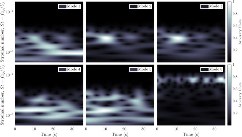
ROVIRA, ENGVALL, AND DUWIG

jet around the x axis. They also mentioned that this frequency depends on α. Yoda and Fiedler [1]
employed flow visualization to describe these oscillations which were reported to be below 1 Hz
at α = 7.5. Nevertheless, the authors mentioned that the type of motion (i.e., rotation, sideways
oscillation, or varying penetration) was not clearly identifiable.
    Lam and Chan [4,5] quantified the effect of the dynamics of counterflowing jets on mean
flow quantities. They used 100 planar laser-induced fluorescence (PLIF) snapshots to obtain the
time-averaged axial and radial penetration lengths with a 4% turbulent intensity in the counterflow
stream. This was done over a range of α from 2.5 to 15. The maximum instantaneous axial and
radial penetrations were observed to be up to 30% and 105% larger than their respective means.
Additionally, the standard deviation of both variables was reported to increase with increasing α.
    Large-scale flow structures of the jet in counterflow and their dynamics were first studied by
Bernero and Fiedler [6]. Two counterflowing jets at α = 3.4 and α = 1.3 were studied employing
particle image velocimetry (PIV) and PLIF. They performed two-dimensional (2D) proper orthog-
onal decomposition (POD) analysis to study the underlying dynamical flow structures. For the
unstable case at α = 3.4, two main modes were reported. The first mode contained radial oscil-
lations, whereas the second mode showed time-varying penetration. Each of the modes presented
distinct frequency peaks at Strouhal numbers St = 0.0266 and St = 0.1155, respectively. Here, the
Strouhal number is St = f x p /U j where f is the frequency, and U j is the jet velocity. However,
higher-order modes did not evidence clear frequency peaks as they contained a broadband frequency
spectrum. Regarding the energy content of the modes, it was reported that the first 10 modes
captured on average 60% of the turbulent kinetic energy present in the flow in the studied range
of α. For lower values of α, the energy content of the first ten modes was higher as the flow state
was more stable. Nevertheless, as pointed out by the authors, these values were much higher in other
flows (i.e., forced shear layers) evidencing the flow complexity of the turbulent jet in counterflow.
    Additional efforts in understanding the dynamics of counterflowing jets were carried out by
Tsunoda and Takei [7]. This study used PLIF to obtain the statistics of a passive scalar field at α =
2.9, 4.0, and 5.1 including centroid position at several jet-normal planes. They reported an increased
radial spread of the jet in counterflow when compared to a free jet issuing into a quiescent stream.
Furthermore, they attributed this increase to the random radial fluctuations of the instantaneous
centroid position. After performing an analysis in Fourier space of the centroid position, results
for peak frequencies were in reasonable agreement with those reported by Bernero and Fiedler [6].
Furthermore, the authors proposed that the first mode (i.e., radial jet oscillations) arose through
similar mechanisms as for the jet flapping observed when a jet is issued into a cavity or a chamber.
    Modal analysis was also employed by Duwig and Revstedt [8] who used three-dimensional (3D)
large eddy simulations (LES) results at α = 2.2 for their analysis. Two similar modes as the ones
reported by Bernero and Fiedler [6] were obtained and revealed that the seemingly 2D flapping
was indeed a 3D jet rotation instead. Nevertheless, these modes were not thoroughly reported as no
energy distribution was presented and only one single value of α was studied. Additionally, their
simulation was performed without employing a turbulent jet inlet condition, which was shown by
Rovira et al. [2] to lead to different results than those reported in the literature.
    Lam [9] used 2D POD analysis on experimental data of counterflowing jets at different values
of α. A fan-shaped region of interest was employed to study modes in the concentration field of
a passive scalar. The most dominant modes reported were consistent qualitatively with the ones
presented by Bernero and Fiedler [6] for low velocity ratios. For higher velocity ratios, however, the
limited size of the interrogation window employed may be obscuring large-scale modes. Moreover,
the down-sampling of the original data used may have led to a reduction in spatial resolution.
    More recently, Sharma et al. [10] studied a slightly different counterflowing jet geometry. They
employed 2D POD on jet-normal velocity field snapshots in three different regions. By analyzing
the energy content of the first modes in the different regions, they conclude that the stagnation
region contains larger coherent structures. Additionally, the contribution of high-order mode on the
turbulence statistics was studied. This way, they report a larger presence of small scale structures in
the jet region compared to the stagnation region.

                                               014701-2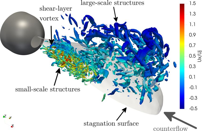
PROPER ORTHOGONAL DECOMPOSITION ANALYSIS OF …

   FIG. 1. Cross-sectional view of the instantaneous axial velocity for the jet in counterflow at α = 5.1 along
with boundary conditions.

    The present review of the available literature evidences an incomplete understanding of the
large-scale dynamics of the jet in counterflow. Although radial jet flapping and oscillating jet
penetration have been shown, studies have mostly been concerned with 2D behavior. 3D POD has
not been thoroughly attempted. Furthermore, only the first two modes have been investigated. There
is consensus that the jet in counterflow is highly complex, yet descriptions of higher-order modes
have not been attempted. Moreover, the relation between fundamental flow patterns and α has not
been investigated in detail. Additionally, no study has motivated their choice of parameters for
POD analysis. Hence, existing results might not be independent of the number of points and/or
snapshots used. The relation between modes and coherent structures has only been performed for
counterflowing wall jets [10]. Currently, there is no link between the two modes showcased in
the literature and the nature of the related flow structures for the jet in counterflow. Finally, no
mention has been made in the literature about the temporal evolution of the modes. Only peak
frequencies have been reported and thus it has not been elucidated if the two modes studied are
stable, periodic, or intermittent. Hence, the large-scale dynamics and coherent structures of the
turbulent jet in counterflow are not yet fully understood.
    The present study aims at addressing all the shortcomings presented regarding the dynamic
behavior of turbulent counterflowing jets. For this, data from previous LES simulations of this flow
configuration by Rovira et al. [2] is employed. Hence, in the present work, 3D POD analysis of
the LES simulations of a turbulent jet in counterflow at several jet-to-counterflow velocity ratios
(α = 2.2, 3.4, 5.1) is performed.

                          II. METHODS FOR SIMULATION AND ANALYSIS
                                         A. Jet in counterflow case
   An overview of the jet in counterflow case employed in the present numerical simulations is
presented. For a detailed explanation, the reader is referred to the work by Rovira et al. [2]. Figure 1
shows the geometry and boundary conditions used in the numerical simulations. The jet nozzle exit
has a diameter of d = 5 mm with all dimensions based on the ones used by Tsunoda and Saruta
[11]. The height of the square duct channel is D = 40d. The distance between the jet inlet and the
counterflow inlet is 60d and the jet inlet is 15d away from the outlet.
   For all cases the simulated working fluid is water and the counterflow speed is fixed to U0 =
−0.21 m/s. Therefore, the jet velocity U j is adjusted to fit the value of α for each case. Three
different values of alpha were studied, α = 2.2, α = 3.4, and α = 5.1 which correspond to Red =
2286, Red = 3533, and Red = 5300, respectively. Here, Red is based on the jet velocity and jet

                                                  014701-3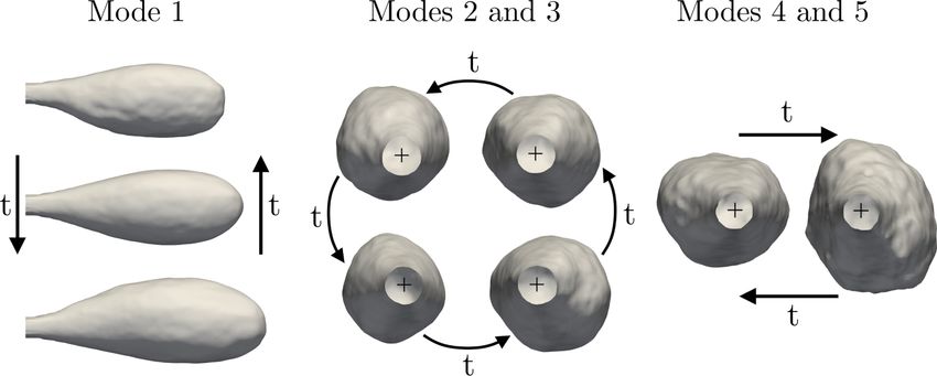
ROVIRA, ENGVALL, AND DUWIG

nozzle diameter. While the counterflow velocity employs a laminar profile, the jet uses a synthetic
eddy method [12] to obtain a turbulent fluctuating velocity profile. All nozzle and channel walls are
modeled by assuming no-slip conditions. The outlet boundary condition for the velocity was set to
zero gradient.
   All cases were simulated using LES in OpenFOAM [13]. The governing equations for an
incompressible flow are as follows:
                                                  ∂ ūi
                                                        = 0,                                         (1)
                                                  ∂xi

                           ∂ ūi        ∂ ūi    1 ∂ p̄     ∂      ∂ ūi
                                 + ū j       =−        +        ν       − τi j
                                                                             SGS
                                                                                  .                  (2)
                           ∂t           ∂x j     ρ ∂xi     ∂x j    ∂x j
    In these equations, ūi and p represent the filtered velocity and pressure, respectively. The
kinematic viscosity is ν, ρ is the density and τiSGSj   is the subgrid-scale stress tensor. The latter
was modeled by the Smagorinsky [14] subgrid-scale model. The pressure-implicit with splitting
operators (PISO) algorithm was used for handling pressure-velocity coupling and linear flux
reconstruction is used for the divergence of velocity. The maximum local Courant number was
Comax = 0.2.
    The independence of the results from the grid resolution was demonstrated by Rovira et al. [2]. In
this previous work, the velocity power spectra for the case with α = 5.1 was presented. Here, a −5/3
slope can be observed for at least one order of magnitude of the power spectrum energy density. This
evidences that the cut-off scales for the LES filter lie well in the inertial subrange of the turbulent
kinetic energy spectrum. The ratio between the cell size and the estimated Kolmogorov length scale
/η was also studied as a mesh quality indicator. Furthermore, the fraction of cells within the
/η < 12 criteria is 99.9% (not shown here). In addition, the results obtained from present LES
simulations were compared with experimental results. A notable agreement was obtained and hence
turbulence levels measured in the experiments were recovered in our simulations. Overall, mean
flow features and turbulent statistics were observed to agree well with the available experimental
literature. This ensures that the data employed for the POD analysis is reliable as the simulations
were capable of accurately describing the flow physics of the turbulent jet in counterflow. The final
mesh used for all simulations had approximately 3 million cells with a normalized minimum cell
element length of d/lmin = 75.

                           B. Overview of proper orthogonal decomposition
    POD analysis has been applied to many jet flow configurations such as a jet in cross-flow [15], a
jet in counterflow [6], a planar jet [16], an annular jet [17], a swirling jet [18], and an underexpanded
jet [19]. It was first introduced from within the field of turbulence by Lumley [20] and is employed
as a tool for statistical analysis of instantaneous flow field variables. A detailed description of the
POD method was provided by Berkooz et al. [21] and a more recent overview was performed by
Taira et al. [22].
    POD decomposes an ensemble of discrete measurement samples into a series of modes, which
constitute an empirical orthonormal basis. These modes represent the optimal projection of the
most important dynamical features of the flow in terms of energy considerations. Each mode can be
described by its relative energy level, spatial distribution, and spectral content. For the POD method,
one must decompose the studied variable of interest as

                                                        N
                                    u(x, t ) = u(x) +         ai (t )φi (x),                         (3)
                                                        i=1

where u(x, t ) is a flow field variable that depends on the spatial vector x and time t, u(x) is the
temporal mean of u(x, t ), φi (x) are the spatial modes and ai (t ) are the time coefficients of the
spatial modes. Note that u(x) is sometimes also referred to as mode 0. In the following, u(x, t ) will

                                                 014701-4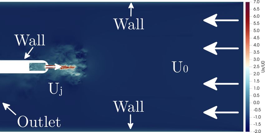
PROPER ORTHOGONAL DECOMPOSITION ANALYSIS OF …

be considered over M spatial points and N time instants. The decomposition in Eq. (3) is defined so
as to optimize the mean square of u(x, t ), usually by an L 2 inner product [22]. Therefore, if u(x, t )
is chosen to be the velocity field, then the turbulent kinetic energy content of the POD modes in the
base would be maximized. In classical POD, the mathematical formulation that yields the spatial
modes can be reduced to an M × M eigenvalue problem [21]. However, as in practical applications
the number of grid points is much larger than the number of time sample (i.e., M  N), the direct
resolution of this form of the eigenvalue problem is computationally expensive. An alternative to
this approach, which is designed to be more computationally efficient, is snapshot POD, also known
as the method of snapshots.
    The method of snapshots was developed by Sirovich [23] to provide a feasible way to handle
POD analysis of 3D flows, which comprise large datasets. Here, the original M × M problem can
be reformulated as an N × N eigenvalue problem by replacing the spatial correlation matrix used in
classical POD by a temporal correlation matrix. The elements of this temporal correlation matrix of
size N × N are given by

                                               1
                                     Ri, j =     u(x, ti ), u(x, t j ),                           (4)
                                               N

where ,  is the L 2 inner product. Solving the eigenvalue problem for the correlation matrix
yields eigenvalues and eigenvectors, which are the mode energies λi ordered decreasingly (i.e.,
proportional to the variance content of their associated mode) and the time coefficients ai . This
is different from classical POD where the resolution of the eigenvalue problem produces the
spatial modes. Therefore, the spatial POD modes must be reconstructed after the N × N eigenvalue
problem has been solved as

                                                1
                                                     N
                                   φi (x) =             ai (t j ) u(x, t j ).                       (5)
                                               λi N j=1

   In the present work, the method of snapshots has been employed to perform the POD analysis
of LES data of simulations of a turbulent jet in counterflow. In order to handle the large 3D
datasets employed [i.e., N ∼ O(1, 000) and M ∼ O(1 000 000)], an in-house parallel C++ code
was developed, which employs the Eigen library [24] for computationally efficient linear algebra
operations.

                                           C. Spectral POD
   Although the method of snapshots is more computationally efficient than classical POD, both
have significant shortcomings. In challenging flow conditions (i.e., intermittent dynamics, weak
coherent structures, or multi-modal interactions) traditional POD approaches fail to produce satis-
factory results. The modes recovered can represent dynamics occurring over a span of time scales,
which hinders insightful interpretations [25].
   Alternatives that tackle this issue by identifying single-frequency modes are spectral methods.
These approaches exchange energy optimality for a frequency restricted analysis. Examples include
discrete Fourier transform (DFT) and dynamic mode decomposition (DMD) [26,27]. Nevertheless,
these methods also have problems with turbulent flows. Due to the shifting nature of frequency
content of large-scale structures and their intermittence, the dynamics of large-scale coherent
structures can rarely be described accurately by a set of discrete frequencies [28].
   These issues were addressed by Sieber et al. [28] by introducing the spectral POD (SPOD)
method. Note that this method must not be mistaken with the one developed by Towne et al. [29] as
both share the same nomenclature. SPOD aims to produce modes which are a tradeoff between the
energetically optimum POD modes and the single-frequency Fourier modes. This is accomplished

                                                  014701-5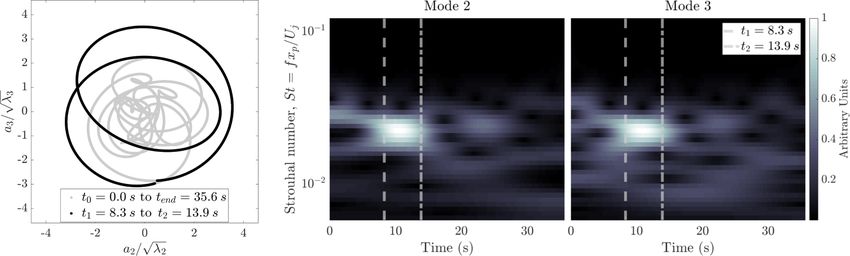
ROVIRA, ENGVALL, AND DUWIG

    FIG. 2. Visualization of the instantaneous jet vortices visualized by isocontours of Q-criterion (Q ∼ 1.5 ×
104 for the large-scale structures and Q ∼ 1.8 × 10⁵ for small-scale structures) and colored by nondimensional
axial velocity. The jet in counterflow depicted has α = 5.1. The time-averaged stagnation surface (isocontour
of axial velocity zero) is represented by a gray transparent isocontour. Both the stagnation surface and the large-
scale structures are clipped by the y = 0 plane for visibility. Additionally, large-scale structures are clipped at
Ux /U j < 0.3 which would otherwise overlap with the small-scale structures. The direction of the counterflow
is also shown for reference.

by applying a filtering operation to the correlation matrix in Eq. (4) as

                                                      Nf
                                           Si, j =            gk Ri+k, j+k ,                                   (6)
                                                     k=−N f

where gk are the elements of the filter vector and N f is the filter width. This operation can be
understood as a way to increase the diagonal similarity of the correlation matrix through a low-
pass Gaussian or box filter. Thus, SPOD allows for interpolation between POD when employing
no filtering and pure Fourier modes with maximum filtering. The remaining procedure for SPOD
analysis is identical to that described in Sec. II b.
   Apart from the filter type (for which the Gaussian shape is preferred), the only choice variable,
which must be defined a priori, is the filter width size N f . Sieber et al. [28] suggest employing
a characteristic time scale of the flow for which the coherent structures that are intended to be
studied present constant dynamical behavior. It must be noted that N f = 1 will imply a filter width
size equal to the difference between the time instants at which two consecutive snapshots were
recorded (assuming snapshots are taken at regular intervals). The main advantage of SPOD is that,
through a soft spectral filtering operation, fluid dynamic structures are less sensitive to noise and are
better separated into different modes. Furthermore, their time evolution is smoother, which allows
for easier identification of paired modes. This notably improves the interpretation of the different
large-scale structures present in the flow.
   The in-house code developed to perform POD also has SPOD capabilities. The additional
operations required incurred in negligible computational costs.

                                     III. RESULTS AND DISCUSSION
                                  A. Visualization of unsteady flow features
   Figure 2 shows a visualization of vortices produced by the jet in counterflow at α = 5.1 by using
the Q-criterion colored by the nondimensional axial velocity. Large-scale and small-scale structures

                                                      014701-6
PROPER ORTHOGONAL DECOMPOSITION ANALYSIS OF …
are represented by two different isocontours of Q ∼ 1.5 × 10⁴ and Q ∼ 1.8 × 10⁵ , respectively.
Additionally, the mean stagnation surface is depicted. Several key features of counterflowing jets
can be observed from this visualization. First, the evolution of coherent structures can be seen. After
exiting the nozzle, the jet generates vortices due to the presence of the shear between the jet and
the counterflow. As can be seen in Fig. 2, these shear-layer vortices have opposing axial velocities
for the top and bottom part of their structure. Hence, they are rotating as well as being transported
downstream. These vortices break down into smaller-scale structures as they are flowing with the
jet in the region where jet momentum dominates. As the jet approaches the stagnation surface,
these small-scale structures become less present and large-scale vortices with tube-like shapes can
be observed. The largest structures exhibit a higher negative axial velocity. Moreover, the largest
vortices appear outside the stagnation surface which implies that it is the jet’s interaction with
the counterflow which produces these structures. These findings are in line with those obtained
by Li et al. [30] and by Sharma et al. [10] for counterflowing wall jets. The instantaneous global
behavior of the jet is also evidenced from Fig. 2. Although the mean velocity is symmetric, the
jet instantaneously follows a preferential direction by bending to one side. This evidences the
instantaneous off-axis large-scale motion of the turbulent jet in counterflow, which has been reported
in the past [2–5]. Both the lower penetration of these instantaneous large-scale jet vortices, as
compared to the stagnation surface, and the deviation of the jet are directly influenced by the two
most dominant modes as presented in Sec. III C. Furthermore, the impact of these modes can be
seen to mainly affect the large-scale structures with negative velocity outside of the time-averaged
stagnation surface.
B. Comparison with previous studies and sensitivity analysis
1. Spatial distribution and energy content
In this section, the results of the present POD analysis of LES simulations of counterflowing
jets are compared with the results available in the literature. The work by Bernero and Fiedler [6]
represents the most thorough investigation of the jet in counterflow employing the POD method and
will thus be the main source for comparison. In their work, the only unstable case studied was at
α = 3.4 for which they report spatial distribution, frequency, and energy content of the obtained
modes. Additionally, the numerical study by Duwig and Revstedt [8] allows for comparison with
a counterflowing jet at α = 2.2, as frequencies for the three main modes are reported. However,
the results presented by Lam [9] do not include modes frequencies and use a fan-shaped region of
interest instead of a rectangular domain, which hinders comparison efforts. Hence, only the former
two works will be employed in the present study. All cases have been analyzed with 3D POD and
additionally, for a more accurate comparison with the data reported by Bernero and Fiedler [6], the
case with α = 3.4 has also been studied with 2D POD.
When performing a POD analysis there are several unknown variables. These include the flow
variable, the number of components of this variable, the extent of the domain of interest, the spatial
resolution, and the temporal resolution (total sampling time and frequency). To the best of the
authors’ knowledge, guidelines or best practices that thoroughly define what these must be are
not currently established. Hence, for an adequate comparison to the literature, the input datasets
employed have been made to be as close as possible to the data available in previous studies.
Additionally, several different spatial and temporal resolutions have been employed to evaluate
how they impact results and to ensure the independence of the results. To do so, linear spatial and
temporal interpolations are employed to obtain the different datasets presented.
Figure 3 shows the spatial distribution of the mean velocity field and the first three modes for 2D
POD with two velocity components at α = 3.4. The visual representation and the coordinate limits
are chosen to closely replicate the ones employed by Bernero and Fiedler [6]. It should be noted that
the domain shown in Fig. 3 is smaller than the complete computational domain employed for the 2D
POD study. For mode 1, a swirling pattern centered around the jet axis is observed, which is slightly
asymmetric for the data from Bernero and Fiedler [6]. This could be due to the relatively small time
014701-7ROVIRA, ENGVALL, AND DUWIG
FIG. 3. Mean velocity (i.e., mode zero) and the first three spatial POD modes for the LES case at α = 3.4.
The 2D POD is performed with two velocity components. It should be noted that the spatial domain shown here
is smaller than the computational domain employed for the present 2D POD study. These coordinate limits and
the accompanying visual representation was employed to replicate that employed by Bernero and Fiedler [6]
to assist the reader in the comparison. In their work, Bernero and Fiedler [6] only present the time-averaged
velocity and the first two modes.
window employed (16 s) for their case as compared to the present results (29 s). Nevertheless, as
they demonstrated in their work when mode 1 is added to the mean velocity field, a radial oscillation
is recovered. In the case of mode 2, Bernero and Fiedler [6] reported the effect of this mode on the
flow dynamics to be a time-varying penetration in the axial direction. Overall, there is a strong
agreement in the spatial distribution of the first two modes when compared to the results obtained
by Bernero and Fiedler [6]. In addition, Fig. 3 shows the spatial distribution of mode 3. This has
been included for the sake of completeness but cannot be compared to experimental results as only
the first two modes were reported by Bernero and Fiedler [6].
As mentioned previously, other POD studies of the jet in counterflow configuration did not
show that their results were independent of the spatial resolution employed. Hence, in addition
to comparing the energy content of the POD modes at α = 3.4 with the literature, the effect of
varying the spatial sampling size and the number of dimensions for POD (i.e., 2D POD and 3D
POD) were studied. Three different spatial resolutions were employed 159 × 90 points, 71 × 41
points and 36 × 21 points. This corresponds to a sampling size normalized with the nozzle diameter
of x/d ≈ 0.1, x/d ≈ 0.2 and x/d ≈ 0.4, respectively. Note that the separation is equal in
all directions such that x = y. For the 3D POD case, the resolution was 159 × 90 × 90 points
with x = y = z. The normalized energy corresponding to the first ten POD modes for all
014701-8PROPER ORTHOGONAL DECOMPOSITION ANALYSIS OF …
FIG. 4. Effect of the spatial sampling size and the dimensions for the POD study (2D or 3D) on the
evolution of the normalised energy corresponding to each POD mode at α = 3.4. All LES results are studied
with either 2D or 3D POD and have a temporal resolution of f ≈ 31 Hz and T = 29 s. They are compared with
the 2D experimental data by Bernero and Fiedler [6] with f ≈ 25 Hz and T = 16 s. Here, f is the sampling
frequency, x/d is the spatial sampling size normalized with the nozzle diameter (note that x = y) and T
is the total sampling time.
cases plus the experimental data reported by Bernero and Fiedler [6] are shown in Fig. 4. All LES
cases were set to have a sampling frequency of f ≈ 31 Hz and the longest possible sampling time,
T = 29 s. The results by Bernero and Fiedler [6] employ a sampling frequency of f ≈ 25 Hz and
a sampling time of T = 16 s. Overall, reasonably good agreement with the experimental data is
obtained when compared to any of the 2D LES cases. Although significant discrepancies can be
observed, with the first POD mode having the largest difference (∼25%), higher-order modes are
notably similar. Furthermore, Fig. 4 shows that the difference in spatial resolution has a minor effect
on mode energy distribution. The maximum discrepancy between our 2D POD cases, which can be
observed for the energy content of mode 1, is smaller than 2% when comparing the values of the
x/d = 0.1 and x/d = 0.4 cases. The higher spatial resolution can capture a larger number of
smaller fluid structures which in turn reduces the overall weight of the energy in the first POD mode.
Nevertheless, as the difference is not significant, coarse POD meshes can be employed without
a notable decrease in precision when obtaining the energy contained in the most dominant POD
modes. Additionally, the difference in the number of dimensions used is seen to have a significant
effect on the energy distribution. When 2D POD is carried out, a single 2D rectangular plane with
two in-plane velocity components per point is used while 3D POD defines a square cuboid domain
with all three velocity components on each point. As can be seen from Fig. 4, employing a 3D
POD would lead to a different energy distribution than the one reported by Bernero and Fiedler [6].
Hence, 3D datasets should not be employed to compare POD mode energies to 2D results.
In addition to spatial resolution, the effects of varying the temporal resolution were also investi-
gated and are shown in Fig. 5. All LES simulation cases presented here are studied with 2D POD
at α = 3.4 and have a normalized spatial sampling size of x/d ≈ 0.1. As can be observed in
Fig. 5 (left), halving the sampling frequency from f ≈ 62 Hz to f ≈ 31 Hz has a negligible effect
on energy distribution as both curves overlap. Halving the frequency again to f ≈ 15 Hz has a
small but noticeable effect on energy distribution (at most ∼4%). However, the effect of choosing
different sampling times has the most substantial impact, as can be seen in Fig. 5 (right). The total
time, T = 29 s was divided equally into two datasets, one from T = 0 s to T = 14.5 s and another
014701-9ROVIRA, ENGVALL, AND DUWIG
FIG. 5. Effect of the sampling frequency (left) and the sampling time (right) on the evolution of the
normalised energy corresponding to each POD mode at α = 3.4. All LES results are studied with 2D POD and
have a spatial resolution of x/d ≈ 0.1. They are compared with the 2D experimental data by Bernero and
Fiedler [6] with x/d ≈ 0.2. Here, f is the sampling frequency, x/d is the spatial sampling size normalized
with the nozzle diameter (note that x = y) and T is the total sampling time.
from T = 14.5 s to T = 29 s. Comparing the resulting energy distributions, notable differences can
be observed. In the first time period, the energy content of the first POD mode is much greater
than in the second period, rising above 16%. Hence, the results from the first period are more in
agreement with the data presented by Bernero and Fiedler [6]. This difference in mode energy
content between the first and second time window could be explained by modes having intermittent
behavior. If modes are intermittent (i.e., not continuously active throughout the temporal evolution
of the jet), then when a particular time period has a higher concentration of these mode events
that mode will show higher energy content. Additionally, the noticeable differences between the
two equally large time-windows presented in Fig. 5 (right) evidence that full convergence has not
been obtained at 14.5 s. Therefore, flow statistics may not be fully converged within the total 29 s
of time-span studied. This is a common problem when carrying out a POD study of LES data.
However, the computational expense incurred by running the simulation for longer still was not
feasible in the present work. Hence, the total sampling time employed here is a compromise between
computational time and convergence.
2. Spectral content and intermittency
To verify the hypothesis of mode intermittency, a continuous wavelet transform of the time
coefficients was performed. This method allows for obtaining the time-resolved spectral content
of a signal by comparing it to shifted and scaled versions of a finite mother wavelet. A thorough
description of wavelet transforms is given by Daubechies [31]. In the present work, a discrete im-
plementation of the continuous wavelet transform using a Morse wavelet with symmetry parameter
equal to 3 is employed. Results for the first three modes at α = 3.4 in both the 2D and 3D POD cases
can be observed in Fig. 6. The gray-scale color represents the relative intensity of the frequency
peak, which is normalized as the Strouhal number based on the mean penetration length and the jet
velocity, St = f x p /U j . The solid white lines represent the peak frequency reported by Bernero and
Fiedler [6]. The white dashed lines represent the range for the peaks observed by Tsunoda and Takei
[7] in the power spectra of the instantaneous jet centroid position.
As predicted, all POD modes presented in Fig. 6 showcase intermittent behavior. This can be
observed from the chaotically alternating bright and dark spots that occur over a range of time
intervals and Strouhal numbers. Contrary to this, ideal continuous (i.e., nonintermittent) modes
would be displayed as a homogeneously bright horizontal narrow band at a constant Strouhal
014701-10PROPER ORTHOGONAL DECOMPOSITION ANALYSIS OF …
FIG. 6. Wavelet transform for the first three POD modes with f ≈ 62 Hz and x/d ≈ 0.1 for (a) 2D and
(b) 3D POD at α = 3.4. The solid white lines represent the peak frequency for each mode reported by Bernero
and Fiedler [6] while the white dashed lines represent the range of frequencies of the main peaks in the power
spectra of the jet centroid for counterflowing jets over the range 2.9 α 5.1 reported by Tsunoda and Takei
[7]. Roman numerals highlight mode events that are discussed in the main text.
number over the entire period studied. Furthermore, considerable agreement with the experimental
results regarding the value of the highest frequency peak is obtained, displayed in the wavelet
transform as the brightest spots. These datasets are presented as solid white lines for data obtained
by Bernero and Fiedler [6] and white dashed lines for the range of frequencies reported by Tsunoda
and Takei [7]. Modes show similar peaks in both the 2D [Fig. 6(a)] and 3D [Fig. 6(b)] POD analysis.
Although the energy content per mode varies considerably between a 2D and a 3D domain as shown
in Fig. 4, the mode frequencies and their evolution in time remain comparable. However, it must be
noted the spatial domains covered by the 2D and 3D POD studies are not equivalent. As the mean jet
is axisymmetric about the jet centerline, the 2D plane would generate a cylinder when rotated along
this axis. Nevertheless, the spatial domain of the 3D POD in Fig. 4 is a square cuboid. Therefore, the
cylindrical domain would have a volume 21% smaller than the square cuboid domain. As the bulk
of the large-scale motions, which contain the highest amount of turbulent kinetic energy, is likely
to occur in the large central region where both cylindrical and square cuboid geometries intersect,
the difference incurred can be neglected. In practice, the observed difference is small and, as the 3D
case has a higher signal-to-noise ratio, it will be used to discuss the specifics of the time-dependent
mode events.
In Fig. 6(b), (I) points at the most intense event (i.e., brightest spots) of mode 1, which
lasts for about ∼5 s and repeats itself three times throughout the time-series. This portrays the
014701-11ROVIRA, ENGVALL, AND DUWIG
FIG. 7. Evolution of the peak value of the Strouhal number for the first six POD modes for several cases of
the jet in counterflow. Results for 2D POD by Bernero and Fiedler [6] and for 3D POD by Duwig and Revsted
[8] are also included for comparison.
intermittent nature of the obtained POD modes. Some frequency modulation is observed but the
overall agreement with Bernero and Fiedler [6], particularly for the latter two spots, is notably high.
The frequency bands presented by Tsunoda and Takei [7], 0.02 St 0.03, contain all individual
event peaks observed. In (II), similar frequency bands to mode 1 can be observed. This suggests
a connection between mode 1 and mode 2 although frequency peaks are slightly higher for mode
2. Intermittency is also evident here. However, (III) points at a large portion of mode 2 which has
a higher frequency content. This local peak has the same frequency as the most intense events of
mode 3. Hence, it can be understood as a spillover of mode 3 into mode 2, which denotes a lack
of frequency separation. This behavior is replicated by the power spectra reported by Bernero and
Fiedler [6] where mode 2 can be seen to have a local peak at the frequency that dominates mode 3.
This is a known and undesirable behavior of classical snapshot POD, which has been reported in
the literature [28]. The interaction between multiple modes leads to multi-frequency spectra as the
snapshot POD method is unable to clearly differentiate between modes. This can be addressed by
employing SPOD. Finally, (IV) marks the main event of mode 3. It is shorter in duration than mode
1 and mode 2 events and repeats itself often but with less intensity throughout the time-series. Again
the peak agrees very closely with the value reported by Bernero and Fiedler [6], St = 0.1155, while
overpredicting the bands defined by Tsunoda and Takei [7], 0.06 St 0.09. Overall, all modes in
both Figs. 6(a) and 6(b) show that mode behavior is notably intermittent for the jet in counterflow.
Although reporting solely maximum frequency peaks paint a biased picture of mode behavior
as it hides intermittency, the evolution of dominant mode frequencies with both mode number
and α is relevant. Compiled results for 3D POD of the present LES cases at α = 2.2, 3.4 and 5.1
along with results by Duwig and Revsted [8] and Bernero and Fiedler [6] are presented in Fig. 7.
As previously reported, agreement with Bernero and Fiedler [6] for maximum frequency peaks
for the first three modes is significant. Additionally, three other higher-order modes are presented
which showcase reasonable agreement, being particularly high for mode 5, and mode 6. When
comparing the present LES case with numerical data obtained by Duwig and Revsted [8], frequency
peaks were again in close agreement. Unfortunately, results for only the first three modes were
014701-12PROPER ORTHOGONAL DECOMPOSITION ANALYSIS OF …
reported in their study. In general, the dominating frequency appears to follow a similar pattern with
increasing mode number, regardless of the value of α. The first modes, which are the largest in
terms of energy content, have similar and relatively low frequencies. For higher-order modes with
less energy content, frequency peaks are higher but broadly comparable. Hence, two groups are
visible: high-energy lower-frequency modes and low-energy higher-frequency modes. Furthermore,
the difference in frequencies between these two groups appears to diminish with increasing α when
using the present normalization. Hence, increasing the strength of the counterflow (i.e., decreasing
α) increases the frequency of the lesser-dominant modes. Therefore, this can be interpreted as the
counterflow having a higher impact on high-frequency mode behavior.
C. 3D SPOD analysis
As relevant features might not be fully revealed by a 2D POD study of the jet in counterflow,
a more thorough study of the 3D POD results has been carried out. The case selected for this
analysis has α = 5.1 which is the highest value among the cases studied. This makes this simulation
more relevant from a practical standpoint as industrial applications requiring efficient mixing utilize
higher velocities. Finally, as has been shown by Rovira et al. [2], the jet in counterflow case with
α = 5.1 agrees particularly well with the results available in the literature.
The present flow configuration has been observed to have a very flat mode energy profile when
studied with 3D snapshot POD (see Fig. 4). This implies that no mode strongly dominates over
the rest and thus a large number of modes are required to accurately describe the motion of
the jet in counterflow. This makes this flow configuration complex and challenging to analyze
with snapshot POD. Additionally, Fig. 6(b) shows that POD modes are intermittent and display
significant frequency modulation due to interaction between modes with similar energy content.
Furthermore, as seen in Fig. 7, the frequency band at which these modes have their peaks is quite
narrow, particularly at α = 5.1. Hence, using snapshot POD on such a flow configuration leads to
poor mode separation and undesirable multi-modal interactions. Therefore, SPOD can be employed
to tackle some of the shortcomings of snapshot POD.
The main two parameters in an SPOD analysis are the type and width of the filter that is applied
to the correlation matrix. In the following study, a Gaussian filter is employed instead of a box filter
as the former has a smoother response [28]. Regarding the filter width size, a value of N f = 366 was
selected to replicate the period of one of the most prominent frequency peaks shown in the velocity
power spectra in Rovira et al. [2]. Higher and lower values for N f were also tested but the selected
value was, for the present case, a trade-off between spectral purity and loss of energy optimality. The
3D SPOD analysis was performed on a total of 3608 snapshots collected over a period of T = 35.6 s
at a sampling frequency of f = 101 Hz and using 106 × 60 × 60 points which yields a normalized
spatial sampling size of x/d = 0.13.
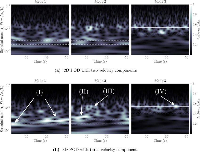
Figure 8 shows the normalized wavelet transform of the first six SPOD modes with N f = 366.
When compared to the results obtained for 3D POD in Fig. 6(b) the effect of SPOD is evident.
It must be noted that a direct comparison between both figures cannot be made as both have
different values of α. Nevertheless, the spectral content of the modes obtained through SPOD
has considerably less noise and smaller frequency bandwidth. Hence, SPOD enables a better
understanding of the key features of the different modes in the frequency space. All modes are
highly intermittent and contain events of different duration and relative intensity, with a spectral
content bound by 0.01 St 0.1. In the following, a detailed explanation of the characteristics of
modes 1 to 5 are presented.
Figure 9 (left) showcases the spatial and temporal effect of mode 1 on the flow field as viewed
from the x-z plane. This figure is generated by selecting relevant time instants of the temporal
evolution of the mean stagnation surface, obtained from the reconstructed flow field created by
the sum of mode 1 and the time-averaged velocity field. As can be seen, this mode represents a
varying axial penetration. However, as observed from the wavelet transform of this mode in Fig. 8,
the frequency at which this oscillating penetration length occurs suffers considerable modulation
014701-13ROVIRA, ENGVALL, AND DUWIG
FIG. 8. Wavelet transform of the first six SPOD modes with filter size N f = 366.
under the period analyzed. With increasing time, the frequency of the most intense event (i.e., the
brightest spot) starting at t = 10 s steadily decreases until stabilizing at around St = 0.01 from
t = 20 s onward. This time-resolved behavior would be lost if only the power spectra of the time
coefficients were reported. The spatial distribution of mode 1 can also be analyzed from Fig. 9 (left).
When compared to the same mode reported by Bernero and Fiedler [6] (although at a different value
of α), the present results for mode 1 display considerably less degree of off-axis displacement. In the
reconstruction by Bernero and Fiedler [6] of the varying penetration mode, the flow field displays
similar oscillating behavior to the mode representing radial jet flapping. This could be explained by
an undesirable multi-modal interaction in their results caused by the fact that snapshot POD is not
able to differentiate between modes as clearly as SPOD can [28].
FIG. 9. (Left) Reconstruction of the temporal evolution of the first SPOD mode visualized by the stagnation
surface viewed on the x-z plane. (Middle) Reconstruction of the temporal evolution of the second and third
SPOD modes visualized by the stagnation surface viewed on the y-z plane. (Right) Reconstruction of the
temporal evolution of the fourth and fifth SPOD modes visualized by the stagnation surface viewed on the y-z
plane. The black arrows indicate the direction forwards in time and the black cross represents the jet centerline.
014701-14PROPER ORTHOGONAL DECOMPOSITION ANALYSIS OF …
FIG. 10. (Left) Phase portrait showcasing the relationship between the temporal coefficient of the second
and third SPOD modes. The solid gray line represents the complete time period from t0 = 0 s to tend = 35.6 s
while the solid black line, which partially covers the gray line, depicts the period between t1 = 8.3 s and
t2 = 13.9 s. (Middle and right) Wavelet transform of the second and third SPOD modes. The vertical gray
dashed lines highlight the time period when the most intense event (i.e., brightest spot) occurs which matches
the period for which the black line in the phase diagram is drawn.
As can be observed in Fig. 8, the spectral content of mode 2 and mode 3 are very similar. This
hints at a relation between both modes. If the effect of each of these modes on the flow field is to
be observed individually, then two different 2D radial jet flapping motions would be recovered, one
for each mode. Although this matches the findings by Bernero and Fiedler [6], access to 3D data
shows that these oscillations occur in orthogonal directions, making modes 2 and 3 a mode pair. The
reconstructed motion of the mode 2-3 pair is shown in Fig. 9 (middle) as viewed from the y-z plane.
This combined mode effectively displaces the most downstream edge of the jet centerline to one
side without bending and then makes it follow a circular rotating trajectory around the undisturbed
jet axis. Overall, the whole jet rotates about an axis different from its own. This type of motion
has been described in the past as jet precession (without rotation) and is distinct from jet swirl
[32]. Nevertheless, this motion is not perfectly consistent nor periodic. To illustrate this, the phase
diagram and wavelet transform of the temporal coefficients of mode 2 and 3 are presented in Fig. 10
(left) and Fig. 10 (middle and right), respectively. In the case of a periodic ideal mode with no
variation in amplitude and a constant frequency, the phase diagram (Lissajous figures) will show a
perfect circle indicating the limit cycle. In a wavelet transform, this limit cycle would be represented
by a thin and homogeneously intense horizontal line. In the present case, the phase diagram shows
that during most of the period studied the trajectory of the time coefficients is rather erratic. This is
marked by a solid gray line. However, between two specific time instants t1 = 8.3 s and t2 = 13.9 s
marked by a solid black line, the phase diagram approximates a circle. Note that the black line
overlaps the gray line. During these more than 5 s, the phase lag between the two modes approaches
π /2. Hence, this pair of modes is describing a single large-scale motion, as their spectral content
is similar in amplitude and frequency but shifted by π /2. This period is delimited in the wavelet
transform by two gray dashed lines and bounds the most intense mode event recorded in the present
time series. Overall, in conjunction with Fig. 9 (middle), Fig. 10 shows that modes 2 and 3 represent
a mode pair with three-dimensional precession and that this motion is intermittent.
Last, the nature of the mode pair formed by modes 4 and 5 can be observed in Fig. 9 (right) as
viewed from the y-z plane. The combined effect of these modes on the reconstructed flow field is
that of alternating stretch in two orthogonal directions. Here, the stagnation surface can be seen to
initially stretch in the horizontal direction and contract in the vertical direction. After some time
the opposite happens in each direction, the stagnation surface stretches in the vertical direction and
contract in the horizontal direction. For this pair, the motion is not perfectly symmetrical as the
stagnation surface displays a slight deviation to one side. Similar to the mode pair 2-3, this motion
is intermittent as can be seen from the wavelet transform of the time coefficient in Fig. 8.
014701-15ROVIRA, ENGVALL, AND DUWIG
IV. CONCLUSIONS
In the present work, a study of the large-scale dynamics of the jet in counterflow has been
performed. By examining the available literature, several open questions regarding this topic have
been evidenced. Through POD analysis of numerical data from LES simulations by Rovira et al.
[2], this study aimed at answering these questions.
Coherent structures in the flow field are investigated using the Q-criterion. Qualitatively,
small-scale structures originating from shear-layer interactions have been seen to develop into
large-scale structures outside the stagnation region. Hence, the interaction between the jet and the
counterflow is deemed to be the driver of the dynamics associated with these structures.
A 2D POD study of the LES simulation of a jet in counterflow case with α = 3.4 is directly
compared with experimental results reported by Bernero and Fiedler [6]. In this comparison, the
spatial distribution, energy content, and spectral content of the modes obtained are observed to
be in substantial agreement. Additionally, the peak mode frequencies obtained for α = 3.4 are
comparable to the experimentally determined frequency bands presented by Tsunoda and Takei [7].
For the case with α = 2.2, peak frequencies for the first three 3D POD modes were substantially in
agreement with those reported in the 3D POD study by Duwig and Revstedt [8].
Besides comparing the present results to previous studies, the effect of varying different spatial
and temporal parameters on the POD analysis of the case with α = 3.4 was studied. First, the
individual energies and spectral content of the modes obtained by 2D and 3D POD were compared.
Despite there being notable discrepancies in the energy levels of the different modes, the frequency
content yielded by both approaches was remarkably similar. Hence, it was concluded that the
appropriate mode frequencies can be captured by 2D POD but this method tends to overestimate
the relative importance, in terms of energy content, of the modes obtained as compared to 3D POD.
Additionally, the impact of different spatial and temporal resolutions was studied by varying the total
number of points in the domain and by modifying the sampling frequency for a fixed sampling time.
It was observed that changing the frequency had a larger effect on individual mode energies than
varying the grid spacing. Nevertheless, the effect of both variations on the overall energy content
remained small. The largest impact on POD results was caused by changing the sampling time. This
analysis was carried out by dividing the total sampling period into two equally large time windows.
Furthermore, the mode energies yielded by these two cases, particularly for the most dominant order
modes, were observed to be notably different. This discrepancy was attributed to uneven spectral
content during the total period analyzed. Furthermore, this was confirmed by the wavelet transform
of the POD time coefficients and revealed intermittency in the behavior of the modes. To the best of
the authors’ knowledge, the intermittent nature of the fundamental large-scale dynamics of the jet
in counterflow is reported here for the first time.
Additionally, a 3D SPOD analysis of the jet in counterflow at α = 5.1 was performed. The
advantages of employing SPOD for the modal analysis of this complex flow configuration, such as a
better signal-to-noise ratio in the spectral content and clearer mode separation, were evidenced. The
effect of the most dominant modes on the flow field was presented through mode reconstruction.
In this way, oscillating penetration, jet precession, and a stretching and contracting motion were
observed to be the main large-scale dynamics of the jet. In all cases, frequency modulation and
intermittency were seen to have a significant effect on jet dynamics. It should be noted, however,
that the physical origin of these phenomena remains unknown. Hopefully, the knowledge presented
in this work aids in the understanding of the large-scale dynamics of this flow configuration and the
design of high mixing efficiency applications.
ACKNOWLEDGMENTS
This work has been funded by Formas (Swedish Research Council for Sustainable Development).
Simulations were performed on resources provided by the Swedish National Infrastructure for
Computing (SNIC) at LUNARC (Lund University) under Project SNIC 2019/3-641 and PDC
014701-16PROPER ORTHOGONAL DECOMPOSITION ANALYSIS OF …
Center for High-Performance Computing (KTH Royal Institute of Technology) under Project SNIC
2019/1-41.
[1] M. Yoda and H. E. Fiedler, The round jet in a uniform counterflow: Flow visualization and mean
concentration measurements, Exp. Fluids 21, 427 (1996).
[2] M. Rovira, K. Engvall, and C. Duwig, Review and numerical investigation of the mean flow features of a
round turbulent jet in counterflow, Phys. Fluids 32, 045102 (2020).
[3] O. König and H. E. Fiedler, The structure of round turbulent jets in counterflow: A flow visualization
study. In Advances in Turbulence 3 (Springer, Berlin, 1991), pp. 61–66.
[4] K. M. Lam and H. C. Chan, Round Jet in Ambient Counterflowing Stream, J. Hydraul. Eng. 123, 495
(1997).
[5] H. C. Chan and K. M. Lam, Statistics of fluctuating dispersion and penetration of a round jet into a
counterflow, edited by T. Huang, J. Turner, M. Kawahashi, and M. Otugen (ASME, 1995) Vol. 229,
pp. 31–38.
[6] S. Bernero and H. E. Fiedler, Application of particle image velocimetry and proper orthogonal decompo-
sition to the study of a jet in a counterflow, Exp. Fluids 29, S274 (2000).
[7] H. Tsunoda and J.-i. Takei, Statistical characteristics of the cross-sectional concentration field in a round
counter jet, J. Fluid Sci. Technol. 1, 105 (2006).
[8] C. Duwig and J. Revstedt, Large-scale dynamics of a jet in a counter flow. In Advances in Turbulence XII
(Springer, Berlin, 2009), pp. 321–324.
[9] K. M. Lam, Application of POD analysis to concentration field of a jet flow, J. Hydro-environ. Res. 7,
174 (2013).
[10] S. Sharma, V. Jesudhas, R. Balachandar, and R. Barron, Turbulence structure of a counterflowing wall jet,
Phys. Fluids 31, 025110 (2019).
[11] H. Tsunoda and M. Saruta, Planar laser-induced fluorescence study on the diffusion field of a round jet in
a uniform counterflow, J. Turbul. 4, N13 (2003).
[12] N. Kornev, H. Kröger, and E. Hassel, Synthesis of homogeneous anisotropic turbulent fields with
prescribed second-order statistics by the random spots method, Commun. Numer. Methods Eng. 24, 875
(2007).
[13] H. G. Weller, G. Tabor, H. Jasak, and C. Fureby, A tensorial approach to computational continuum
mechanics using object-oriented techniques, Comput. Phys. 12, 620 (1998).
[14] J. Smagorinsky, General circulation experiments with the primitive equations, Monthly Weather Rev. 91,
99 (1963).
[15] K. E. Meyer, J. M. Pedersen, and O. Özcan, A turbulent jet in crossflow analysed with proper orthogonal
decomposition, J. Fluid Mech. 583, 199 (2007).
[16] S. V. Gordeyev and F. O. Thomas, Coherent structure in the turbulent planar jet. Part 1. Extraction of
proper orthogonal decomposition eigenmodes and their self-similarity, J. Fluid Mech. 414, 145 (2000).
[17] B. Patte-Rouland, G. Lalizel, J. Moreau, E. Rouland, Flow analysis of an annular jet by particle image
velocimetry and proper orthogonal decomposition, Meas. Sci. Technol. 12, 1404 (2001).
[18] K. Oberleithner, M. Sieber, C. N. Nayeri, C. O. Paschereit, C. Petz, H.-C. Hege, B. R. Noack, and
I. Wygnanski, Three-dimensional coherent structures in a swirling jet undergoing vortex breakdown:
Stability analysis and empirical mode construction, J. Fluid Mech. 679, 383 (2011).
[19] V. Vuorinen, J. Yu, S. Tirunagari, O. Kaario, M. Larmi, C. Duwig, and B. J. Boersma, Large-eddy
simulation of highly underexpanded transient gas jets, Phys. Fluids 25, 016101 (2013).
[20] J. L. Lumley, The structure of inhomogeneous turbulent flows, in Atmospheric Turbulence and Radio
Wave Propagation (Nauka, Moscow, 1967).
[21] G. Berkooz, P. Holmes, and J. L. Lumley, The proper orthogonal decomposition in the analysis of
turbulent flows, Annual Review Fluid Mechanics 25, 539 (1993).
014701-17You can also read