High-Resolution Lightning Detection and Possible Relationship with Rainfall Events over the Central Mediterranean Area - MDPI
←
→
Page content transcription
If your browser does not render page correctly, please read the page content below
remote sensing
Article
High-Resolution Lightning Detection and Possible
Relationship with Rainfall Events over the Central
Mediterranean Area
Guido Paliaga 1, *, Carlo Donadio 2 , Marina Bernardi 3 and Francesco Faccini 1,4
 1    CNR IRPI Research Institute for Geo-Hydrological Protection, 10135 Torino, Italy
 2    DiSTAR—Department of Earth Sciences, Environment and Resources, University of Naples Federico II,
      University Campus of Monte Sant’Angelo, 80126 Napoli, Italy
 3    CESI S.p.A.—SIRF and Meteo Laboratory ISMES division, 20134 Milano, Italy
 4    DISTAV Department of Earth, Environmental and Life Sciences, University of Genoa, 16132 Genova, Italy
 *    Correspondence: guido.paliaga@irpi.cnr.it

 Received: 30 April 2019; Accepted: 3 July 2019; Published: 5 July 2019

 Abstract: Lightning activity is usually associated with precipitations events and represents a possible
 indicator of climate change, even contributing to its increase with the production of NOx gases.
 The study of lightning activity on long temporal periods is crucial for fields related to atmospheric
 phenomena from intense rain-related hazard processes to long-term climate changes. This study
 focuses on 19 years of lightning-activity data, recorded from Italian Lightning Detection Network SIRF,
 part of the European network EUCLID (European Cooperation for Lightning Detection). Preliminary
 analysis was dedicated to the spatial and temporal assessment of lightning through detection in the
 Central Mediterranean area, focusing on yearly and monthly data. Temporal and spatial features have
 been analyzed, measuring clustering through the application of global Moran’s I statistics and spatial
 local autocorrelation; a Mann–Kendall trend test was performed on monthly series aggregating the
 original data on a 5 × 5 km cell. A local statistically significant trend emerged from the analysis,
 suggesting possible linkage between surface warming and lightning activity.

 Keywords: lightning; clustering; flood; Mediterranean

1. Introduction
      In recent years, research interest in lightning has increased thanks to improved monitoring
technology, which makes a huge amount of high-precision data available on an increasing temporal
range. Interest is mainly related to scientific aspects, nature and the development of the phenomenon
itself [1,2], associated hazards [3–7], the relationship between weather and climate features [8–10],
and innovation in detection approaches [11,12]. In fact, cloud–ground lightning causes damage to
buildings, infrastructures, and facilities, wildfires, and even casualties [1]. On a global scale, thousands
of deaths and injuries are caused by lightning every year, and occurrence is more frequent in developing
countries where, on average, 150–200 casualties are registered per year. However, lightning causes
many losses even in industrialized western countries: in the United States, about 100 people die of a
lightning stroke every year [13].
      In this paper, we use the term “lightning” to generically indicate atmospheric discharges correlated
to convective activity, while we use the term “flash” to indicate the more specific process of a discharge
forming from a stepped-leader–return-stroke process (for cloud-to-ground events). Each flash can
present one or more single currents named “strokes”, usually flowing in the same channel as the first
stroke, and sometimes striking the ground at different points [1]. For cloud-to-cloud discharges we

Remote Sens. 2019, 11, 1601; doi:10.3390/rs11131601                       www.mdpi.com/journal/remotesensing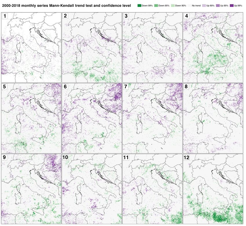
Remote Sens. 2019, 11, 1601                                                                          2 of 20

generically use the term “cloud-cloud events”, without distinction between cloud-to-cloud, intracloud,
or cloud-to-air processes.
      The Mediterranean Sea is one of the most intense electric-activity areas of the Northern
Hemisphere [14] and, consequently, is one of the highest meteohydrological-risk areas of the world
due to its highly vulnerable elements. On average, lightning claims between 5 and 10 victims per year
per country [15].
      Several studies approached the spatial and temporal distribution of lightning in the Mediterranean
region: activity largely prevails on the sea surface in winter and on land in spring and summer [16–20],
following the seasonal cycle of surface warming. The identification of convective systems into complex
meteorological structures such as hurricanes [21], mesoscale systems, and local thunderstorms needs
continuous lightning monitoring. Adequate surveying is also crucial for civil-protection action plans
and to adopt appropriate risk-mitigation strategies.
      In the Mediterranean area, floods and flash floods with disastrous consequences are often
associated with intense rain events [6,7]. Considering the period starting from the year 2000, 73
floods/flash floods occurred [22] along all the seasons, but with higher frequency (over 45%) in October
and November. The Italian peninsula and the French Mediterranean coastline are among the most
affected areas, with 23 and 11 events, respectively [22], happening during the entire year and primarily
in fall (over 56%). In the last 50 years, in the central Liguria region, one of the most exposed areas,
some authors [23,24] evidence that floods have progressively assumed flash-flood features due to
rainfall-event duration, from 3–12 h to 24–72 h.
      The relationship of lightning with climate change has largely been discussed [21,25,26], and
many authors agree in considering a positive correlation between increasing surface temperatures and
lightning activity [27–29], but such correlation does not find general agreement. Finney et al. [30] expect
a reduction in lightning to be correlated with an increase in surface temperature due to modifications
in ice-cloud fluxes. Thus, a longtime series study appears crucial for a deeper comprehension of
the relationship between lightning and climate change, and of the relationship with natural hazards.
Nowadays, high-precision lightning ground detection systems allow the monitoring of long-distance
activities, even on a large scale, contributing to large databases on wide geographical areas [19,31,32].
Some global-scale databases are committed to the spatial distribution of thunderstorm cells [33].
      Some studies focused on studying the relationship between lightning and surface morphology
and land use: generally, there is good correlation with orography [34], especially in the presence of
steep slopes that enhance the rapid uplift of unstable air masses, while even urbanization appears
to affect the local increase of lightning [35]. Orographic influence is particularly important in coastal
areas, as underlined by many authors [1,5].
      Many other research efforts [1] have been devoted to studying atmospheric factors driving
lightning activity, and stressing the connection between lightning and available convective potential
energy. If surface warming is the basic element that is strictly correlated with atmospheric instability,
more work is needed to investigate the relationship between lightning, sea-surface temperature, and
land temperature, like the work of Kotroni and Lagouvardos [9].
      This research focuses on giving a preliminary characterization of cloud–ground strokes across the
Mediterranean area surrounding the Italian peninsula based on the Italian Lightning Detection System
SIRF, which is part of the European EUCLID network and uses ground-based sensors. The 19-year SIRF
database (2000–2018) was used to analyze the strokes’ spatial and temporal distribution in the central
Mediterranean area in order to: a) integrate existing studies with longer annual and monthly series,
supporting further meteorological and climatic research; b) assess a possible relationship between
surface warming and lightning activity or a possible trend in time, which would contribute to assessing
future scenarios of the eventual increase of extreme meteorological events.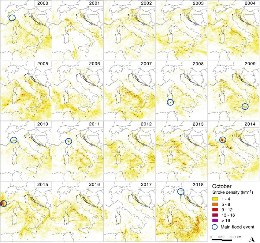
the coastal zone, within 10 km from the seashore, is about 8% of the total land area.
      The area (Figure 1) includes the entire Alps and Apennines chains, the Po plain, the western
Balkan peninsula, and the northeast termination of the Atlas Mountains; altitudes are between sea
level and 4810 m.
RemoteAccording
       Sens. 2019, 11,to1601
                          the Köppen [36] classification, the type of climate ranges between alpine, boreal,   3 of 20
warm temperate, and arid [37]. General atmospheric circulation is dominated by humid western
currents. with the seasonal influences of the Azores and North African anticyclones; in winter, the
2. Materials
central         and Methods
         Mediterranean        is sporadically affected by currents from the Balkans or from Scandinavia [38].
The strong thermic contrast between air masses in such a complex and heterogeneous area
2.1. Area of Interest
contributes to generating high electric activity and heavy rains with a high-intensity rate: the highest
valueThe    areamm/h
        of 180      under    study
                           was        is centered
                                measured    in 2011over    thecentral
                                                      in the    ItalianLigurian
                                                                         peninsula  (Figure (Point
                                                                                Apennines    1) and1 incovers about
                                                                                                         Figure  1B),
2,000,000
when a flashkm2 ;flood
                   it is defined
                           causedby    longitude 4.04128E,
                                    6 casualties   [39], but alatitude
                                                                rate of34.6403N;
                                                                         140 mm/hand  longitude
                                                                                    was  reached 21.5229E,  latitude
                                                                                                   in the same   area
48.6584N.
during a 2014The surface     is almost
                   flash-flood     eventequally
                                          [40,41].distributed
                                                    In the lastbetween
                                                                20 years,land  and sea,
                                                                           several      52%
                                                                                   floods    andflash
                                                                                           and    48%,floods
                                                                                                        respectively;
                                                                                                              hit the
the coastal
whole         zone,
        Italian        within 10
                 peninsula         km from the seashore, is about 8% of the total land area.
                                [22].

     Figure         Studied area and annual
     Figure 1. (A) Studied              annual stroke mean per square km calculated for the 2000–2018
                                                                                                    2000–2018 period;
     (B) higher  densities along:  1. the central Liguria   coastline, 2. (blue line), the Tyrrhenian
     (B) higher densities along: 1. the central Liguria coastline, 2. (blue line), the Tyrrhenian      coastline, 3. the
                                                                                                           coastline,  3.
     northern   Adriatic
     the northern        Sea, Sea,
                   Adriatic   4. Northeast   Italy,Italy,
                                   4. Northeast     5. the5.Capodistrian   peninsula,
                                                             the Capodistrian           6. Provence
                                                                                 peninsula,          in France,
                                                                                             6. Provence        7. (red
                                                                                                          in France,   7.
     line), the Central Italian Alps, 8. (red line) the Apennines, and 9. inner Corsica. Other cited areas: 10.
     Tyrrhenian Sea, 11. Sicily, 12. Sardinia, 13. northern Atlas, and 14. the western Balkan peninsula.

     The area (Figure 1) includes the entire Alps and Apennines chains, the Po plain, the western
Balkan peninsula, and the northeast termination of the Atlas Mountains; altitudes are between sea
level and 4810 m.
     According to the Köppen [36] classification, the type of climate ranges between alpine, boreal,
warm temperate, and arid [37]. General atmospheric circulation is dominated by humid western
currents. with the seasonal influences of the Azores and North African anticyclones; in winter, the
central Mediterranean is sporadically affected by currents from the Balkans or from Scandinavia [38].
The strong thermic contrast between air masses in such a complex and heterogeneous area contributes
to generating high electric activity and heavy rains with a high-intensity rate: the highest value of
180 mm/h was measured in 2011 in the central Ligurian Apennines (Point 1 in Figure 1B), when a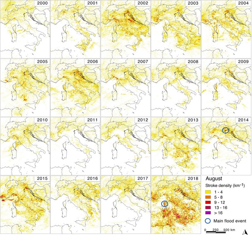
Remote Sens. 2019, 11, 1601                                                                            4 of 20

flash flood caused 6 casualties [39], but a rate of 140 mm/h was reached in the same area during a
2014 flash-flood event [40,41]. In the last 20 years, several floods and flash floods hit the whole Italian
peninsula [22].

2.2. Dataset
      The lightning data used in this study were provided by the Italian Lightning Location System
(SIRF), owned by CESI (Italian Electrotechnical Experimental Center) S.p.A. SIRF covers the entirety
of Italy and Italian seas, with homogeneous performances. SIRF is the Italian member in EUCLID, a
cooperation between national Lightning Location Systems (LLS) operators who joined their systems in
one larger and uniform pan-European network. Thanks to this cooperation, lightning data over all of
Italy and the bordering seas have been continuously located and archived since 2000, not only with the
contribution of SIRF’s own national sensors, but potentially with the contribution of more than 140
sensors over Europe, mainly involving around 30 sensors over Italy and the border countries in data
calculation [42,43].
      Both SIRF and EUCLID are based on the most recent and precise available technology for lightning
detection, with sensors using a combined method of calculation (time of arrival plus direction finding)
for the impact point on the ground. A sophisticated algorithm of waveform recognition is used to
discriminate between cloud–ground and cloud–cloud events.
      Each lightning is detected by multiple sensors in the LLS; information coming from each sensor is
received and elaborated by central analyzers to calculate the main parameters for each lightning strike:
the point of impact on the ground, the date and time of impact, peak current amplitude and polarity,
and type (cloud–ground or cloud–cloud). The network is able to detect each stroke of a cloud–ground
flash event, with its own characteristics, and each stroke is saved in the LLS database, available for
subsequent analysis.
      An algorithm assigns each stroke to a flash event if it is at a distance of less than 10 km and 1 s from
the first event, with an interstroke time of less than 500 ms; each flash is saved in a separate database.
      The network EUCLID performances have been extensively analyzed over the last decade against
ground-truth data collected by either direct measurements on Gaisberg Tower or high-speed video
and field recording system (VFRS). The resulting Detection Efficiency (DE) was determined to be 97%
for flashes containing at least one stroke with a peak current greater than 5 kA, and 80% for strokes
with peak currents greater than 10 kA [44]. The median value of absolute location accuracy (LA) was
measured at Gaisberg Tower in 2014 to reach a median value of 90 m, which is consistent with the
results obtained at larger scales based on VFRS data [39]. SIRF being homogeneous in technology,
calibration, and mean baseline with the rest of the EUCLID network, these performances can also be
inferred for the SIRF system.
      The performances mentioned here for the SIRF system are homogeneous all over Italy and the
bordering seas. The Adriatic Sea being narrow enough, sensors on both the Italian and the Balkan side
assure the same kind of coverage and performance over its surface. The western side of the Italian
Mediterranean waters under analysis are covered by sensors of the Italian mainland, Sardinia, Sicily,
Corsica, and the Balearic Islands, presenting the same performance level from Sardinia toward the
east. On the other hand, south of the Italian coast, in the absence of more sensors, one may expect
degrading performance further from the coast [43]. Although a limited part of the area under study is
involved, this may be considered a limitation of the present study.
      In this work, we used cloud–ground stroke data, with no filter on peak current. The aim of
the study was to provide preliminary analysis of 19 years of measurements, between 2000 and 2018,
detected and located by SIRF and EUCLID in the Italian basin. The database includes a total of more
than 67 million cloud–ground strokes.
      Analysis was performed aggregating (counting) stroke impact points in space, using a
homogeneous 1 × 1 km grid. This is sensible due to extreme precision of the LLS in localization, with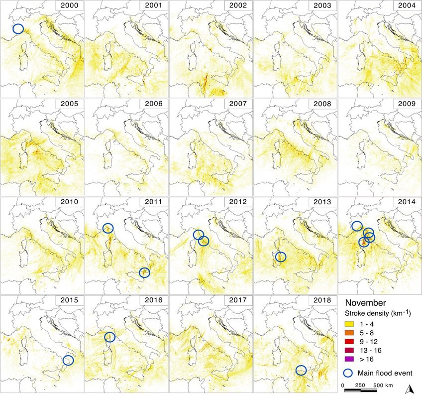
Remote Sens. 2019, 11, 1601 5 of 20
mean location accuracy being much lower than 1 km. Due to computational limits, data were then
grouped in a 5 × 5 km grid to perform cluster analysis (per year or per month).
2.3. Methodology
Considering the peculiar nature of lightning, spatial autocorrelation analysis was performed on
monthly and yearly aggregated data through global Moran’s I statistics, which gives a measure of
data clustering. The basis is given by Tobler’s first law of geography [45,46] that states: “everything is
related to everything else, but near things are more related than distant things”. Then, global Moran’s
I statistics [47,48] transpose the autocorrelation concept to spatially distributed data, measuring spatial
dependency. Moran’s I index is defined as follows:
P P
n i j Wijxi − X x j − X
I= P P 2 (1)
j Wij
i
P
i xi − X
where:
n is the number of geographic entities, that is, the number of cells;
xi is the spatial feature at the location I, that is, the count of stroke per cell;
X is the xi mean value;
Wij is the spatial weight between features i and j;
Calculations were done using inverse distance for the weight matrix with a Euclidian metric;
results were tested at 99% confidence level, as the null hypothesis was the random spatial distribution
of strokes.
Index I may assume values in the range of [−1, 1], extremes corresponding, respectively, to
situations of total dispersion and total clustering, and the 0 value to total randomness. Results of
monthly and yearly calculations are presented in the following paragraphs.
In addition, spatial local autocorrelation was performed in order to evaluate local clustering
through the Getis–Ord local statistic [49] that is defined as follows:
Pn Pn
j=1 Wi,j x j −X
j=1 xi,j
G∗i = (2)
P 2 12
1
n nj=1 Wi,j
2 − n
P
S n−1 j=1 W i,j
n
1X
X= xj (3)
n
j=1
1
n
1 X 2
2
S = x2j − X (4)
n
j=1
where:
n is the number of geographic entities, that is, the number of cells;
x j is the attribute for spatial feature i, that is, the count of stroke per cell;
X is the x j mean value;
Wij is the spatial weight between features i and j;
Calculation was performed in ArcGIS (ESRI. Redlans, CA, USA) using inverse distance for the
weight matrix with a fixed threshold value of 30 km and with a Euclidian metric; the combination
of the obtained z-score and p-value allowed to identify a confidence level of 90%, 95%, and 99%, as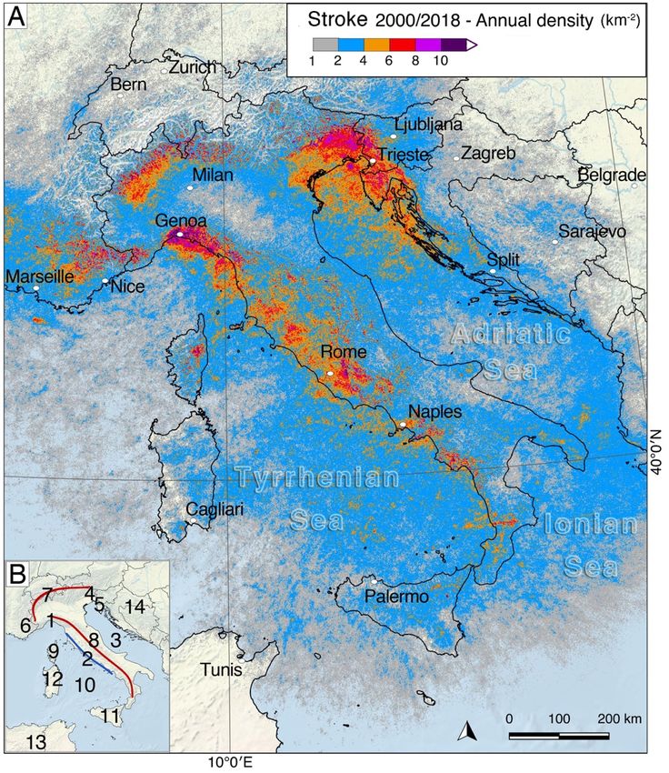
Remote Sens. 2019, 11, 1601                                                                          6 of 20

indicated in Table 1. This approach allows to identify local clusters of lightning strokes; preliminary
statistical first evaluations are shown in the present work.

                         Table 1. Confidence level as a combination of z-scores and p-values.

                              z-Scores                 p-Value             Confidence Level
                       z < −1.65 or z > 1.65       0.05 < p < 0.10                90%
                       z < −1.96 or z > 1.96       0.01 < p < 0.05                95%
                       z < −2.58 or z > 2.58          p < 0.01                    99%

     In order to assess a possible temporal trend, the nonparametric Mann–Kendall test [50,51] was
performed at a spatial scale of a 5 × 5 km grid. Every monthly-series cell was tested and the results
mapped in order to identify areas with statistically significant increasing or decreasing strokes within
the studied period, considering three confidence levels: 90%, 95%, and 99%. The calculation was
performed for every monthly series through the 19 years of measurements, and results are shown in
the following paragraph.

3. Results

3.1. Temporal Distribution
     The statistics in Figure 2A show the mean, maximum, and minimum total number of cloud–ground
strokes per month over the whole geographic area of interest, calculated over the 19-year period: mean
higher counts occurred in August and September, followed by June, July, and October according to the
seasonal climate cycle. May and November may be considered as transitional periods from/towards
the low activity that develops between December and April. Peak count in maximum values was
reached in August. Considering the mean values, differences between the highest (August) and lowest
(January) activity period were about 16 times. The maximum value in the series, registered in August,
is more than three times the mean value of the same month, and correspond to August 2018.
     Figure 2B shows the total number of cloud–ground strokes counted per each year over the whole
area of interest for the entire period under study: values are quite variable from one year to the other
and look dominated by the high count that occurred during 2018, which was more than twice higher
than the mean value of the entire period. In the same figure, the results of global Moran’s I statistics are
shown: values are always high (I > 0.8), denoting strong spatial data clustering along the whole series.
The year 2018, with the highest number of strokes, shows a relatively low value of I, indicating more
diffuse activity in the area. In Figure 2B, the linear trend for number of strokes per year is also shown:
the high variability, strongly influenced by the 2018 value, did not show an increasing trend that would
need to eventually be assessed in further measurement years. A statistic of monthly extremes in stroke
counts per year is shown in Figure 2C: 2018 appears to be singular again, including maximum values
for May, June, August, and October, that is, most of the higher-activity period. Maximum values
for the remaining months were registered in the 2001–2007 period, while the minimum values are
concentrated in the central part of the series between 2007 and 2013.
     Figure 3 shows the monthly series, the total number of cloud–ground strokes per each month
of each year, together with the respective global Moran’s I values; the mean value and the linear
trend are shown as well. The large variability of lightning-stroke activity is evident for every monthly
series, with a single month value frequently twice or three times higher than the monthly mean. This
tendency is particularly evident in August when, in 2018, the total stroke count was three times higher
than the mean value, while in 2011 and 2012 the respective counts were about one-third of the mean.
This extreme variability is always in agreement with the high value of Moran’s I, which means that
clustering is present anyway; even in August 2018, diffuse high activity presented a high clustering
level. An exceptionally high number of lightning in 2018 months occurred even in May and October,
denoting a general tendency for the entire year.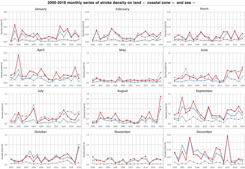
Remote Sens. 2019, 11, 1601                                                                                     7 of 20
 Remote Sens. 2019, 11, x FOR PEER REVIEW                                                                     7 of 21

                  (A) Minimum, maximum, and mean
       Figure2.2. (A)
      Figure                                      mean monthly
                                                       monthlycloud–ground
                                                                 cloud–groundstroke
                                                                                strokecounts.
                                                                                        counts.(B)
                                                                                                (B)Yearly
                                                                                                    Yearlycounts
                                                                                                           counts
      ofofstrokes
           strokesand
                   andglobal
                        globalMoran’s
                               Moran’s II values;
                                          values; mean
                                                  mean for total period
                                                                 period and
                                                                        and linear
                                                                            linear trend.
                                                                                    trend. (C)
                                                                                            (C)Monthly
                                                                                               Monthlyextreme
                                                                                                         extreme
       valuesfor
      values   forthe
                   thetotal
                       totalperiod.
                            period.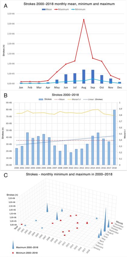
with a single month value frequently twice or three times higher than the monthly mean. This
  tendency is particularly evident in August when, in 2018, the total stroke count was three times
  higher than the mean value, while in 2011 and 2012 the respective counts were about one-third of the
  mean. This extreme variability is always in agreement with the high value of Moran’s I, which means
  that Sens.
Remote clustering
             2019, 11,is  present anyway; even in August 2018, diffuse high activity presented a high
                       1601                                                                                        8 of 20
  clustering level. An exceptionally high number of lightning in 2018 months occurred even in May
  and October, denoting a general tendency for the entire year.
      More
       Moregenerally,
               generally,  and comparing
                              and  comparingthe monthly   series,series,
                                                 the monthly       high variability in monthly
                                                                         high variability         totals was
                                                                                             in monthly       registered
                                                                                                            totals  was
  registered both during the high-activity seasonal period and in low and transitional ones. Global I
both   during   the   high-activity    seasonal   period  and   in  low  and  transitional   ones.   Global   Moran’s
always
  Moran’sdenotes
            I always clustering   in the data,
                        denotes clustering   in but  values
                                                the data, butare lowerare
                                                               values    and  more
                                                                           lower  andvariable  for low for
                                                                                       more variable     stroke
                                                                                                            lowactivity
                                                                                                                 stroke
periods,
  activity denoting      a general ahigher
            periods, denoting               clustering
                                      general            tendency from
                                                higher clustering           June from
                                                                      tendency   to October,
                                                                                        June to with  the exception
                                                                                                   October,   with theof
August    2018.
  exception   of August 2018.
      AAlinear
          lineartrend
                   trendis is
                            drawn
                              drawn onon
                                       every  monthly
                                          every         diagram
                                                  monthly   diagrambut,but,
                                                                        again,  due to
                                                                             again, duethetogreat  variability
                                                                                             the great         of values
                                                                                                         variability  of
invalues
    everyinseries,
             everyresults
                     series,do   not show
                              results do notany
                                              showsignificant long-term
                                                      any significant      tendency.
                                                                       long-term   tendency.

      Figure3.3.Monthly
     Figure     Monthly counts
                         counts of
                                 of cloud–ground strokes and global Moran’s
                                                                     Moran’s II values,
                                                                                values,the
                                                                                        themean
                                                                                           meanfor
                                                                                                forthe
                                                                                                    thetotal
                                                                                                        total
      period, and the linear trend  in the total measurement period.
     period, and the linear trend in the total measurement period.

     The
      Theresults
           results of
                    of the
                        the Mann–Kendall
                            Mann–Kendall trend test are
                                                      are shown
                                                          shown in in Figure
                                                                       Figure 44 for
                                                                                  for every
                                                                                       everymonthly
                                                                                            monthlyseries.
                                                                                                    series.
Increasing
 Increasingtrends
             trendsininthe
                         the19-year
                             19-yearmeasurements
                                    measurements are
                                                  are identified
                                                       identified as follows:
 •    January: along the French coastline and the North African coastline, in the sea west to Sardinia
•    January: along the French coastline and the North African coastline, in the sea west to Sardinia and
      and Corsica, in the sea between Corsica and Ligurian and in the central and northern
     Corsica, in the sea between Corsica and Ligurian and in the central and northern Tyrrhenian Sea;
      Tyrrhenian Sea;
•    February: in the sea surrounding Corsica and along the Balkan coastline;
•    March: in southern Italy, in Sicily, and sporadically along the Apennines and the Tyrrhenian Sea;
•    April: along the French coastline, the central–western Alps, in the strip North of the Alps, and in
     the inner south Balkans;
•    May: in the northern and central inner Balkans, in North–Central and East Italy, in the western
     Alps, and sparsely in the central and northern Tyrrhenian Sea;
•    June: in the northern and central inner Balkans, along the western, central, and eastern Alps, in
     the central and northern Adriatic Sea, in the sea surrounding Corsica, in Provence, and in the sea
     west of Corsica and Sardinia;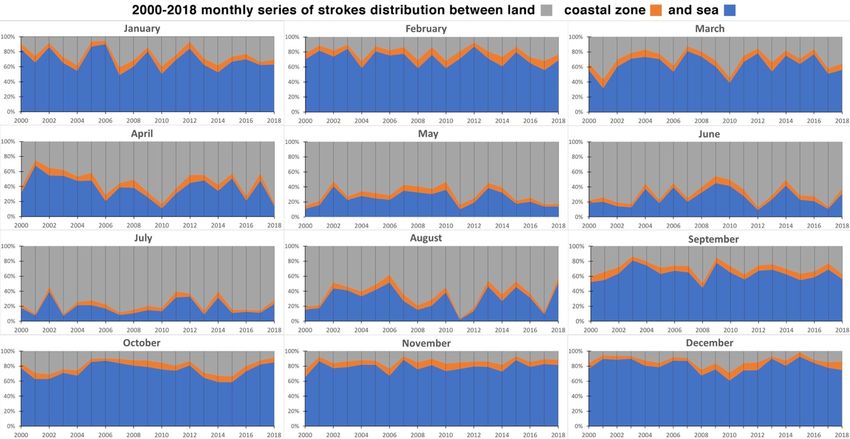
Remote Sens. 2019, 11, 1601                                                                                              9 of 20

•     July: in the northern and central inner Balkans, in the Tyrrhenian and Adriatic south of Italy, in
      inner Corsica, and along the French coastline and facing the sea;
•     August: in the northern and central inner Balkans, in the northern Adriatic Sea, and in the eastern
      and northern Alps;
•     September: in the northern and central inner Balkans, along the central Balkan coastline, northern
      to western Liguria region, and in the western extreme of North Africa in the study area;
•     October: in the central Tyrrhenian Sea and northern to western Sicily, in Africa comprising the
      study area, along the French coastline, and facing the sea;
•     November: sporadic areas in the sea surrounding Corsica and in the sea south of Italy;
•     December: a small and limited area only emerged in the central Adriatic Sea.
Remote Sens. 2019, 11, x FOR PEER REVIEW                                                                                10 of 21

       Figure4.4.Spatial
      Figure      SpatialMann–Kendall
                         Mann–Kendall trendtrend test
                                                  test for
                                                        for the
                                                             themonthly
                                                                monthly series
                                                                         series in
                                                                                 inthe
                                                                                    the2000–2018
                                                                                        2000–2018 period
                                                                                                    period with
                                                                                                              with 90%,
                                                                                                                     90%,
      95%,
       95%,and
            and99%99%confidence
                       confidencelevel.
                                  level.1:1:January;
                                             January;2:2:February;
                                                           February;3:3:March;
                                                                        March;4:4:April;
                                                                                    April;5:5: May;
                                                                                               May;6:6: June;
                                                                                                         June; 7:
                                                                                                               7: July;
                                                                                                                   July; 8:
                                                                                                                         8:
      August;  9: September;  10: October;   11: November;      12: December.
       August; 9: September; 10: October; 11: November; 12: December.

      Decreasing
 3.2. Spatial      trends mainly in February, April, May, September, November, and December in the
              Distribution
southern Tyrrhenian Sea, in the northern African coast, and in the sea south to Sicily. Sporadic reduction
areas Analysis
       were even ofpresent
                    a large amount  of data
                            in northern Italyallowed
                                              and theto point out spatial
                                                      surrounding   areas features of cloud–ground
                                                                           in October and November.strokes
 along the 19 years of measurements. Preliminary visual analysis was performed, while a more
 statistical–mathematical approach will be developed in future studies.
       Figure 1 shows the mean stroke density per square km over each year: there are some differences
 in stroke patterns from year to year depending on the meteorological behavior in that year.
 Nonetheless, some areas were consistently more exposed to strokes, as can also be inferred from
 Figure 1: higher values were localized in the northeastern part of Italy together with the interior of
 the Capodistrian peninsula along the northern Tyrrhenian coastline, that is, the central and eastern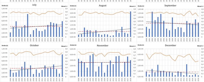
Remote Sens. 2019, 11, 1601                                                                          10 of 20

3.2. Spatial Distribution
      Analysis of a large amount of data allowed to point out spatial features of cloud–ground strokes
along the 19 years of measurements. Preliminary visual analysis was performed, while a more
statistical–mathematical approach will be developed in future studies.
      Figure 1 shows the mean stroke density per square km over each year: there are some differences
in stroke patterns from year to year depending on the meteorological behavior in that year. Nonetheless,
some areas were consistently more exposed to strokes, as can also be inferred from Figure 1: higher
values were localized in the northeastern part of Italy together with the interior of the Capodistrian
peninsula along the northern Tyrrhenian coastline, that is, the central and eastern Liguria region of
Italy, and along the western–central Alps. Other areas of high stroke density were located in the
southern slopes of the Maritime Alps, in Provence, in Corsica, and in the central Tyrrhenian–Italian
border (western side of the Apennines chain).
      In Figures 5–7 the series for August, October, and November are shown, displaying the spatial
distribution of strokes in various months. Great variability in activity and clustering appears evident
even in the monthly series. In the same figures, the main flood events [22] that happened in the
corresponding months are highlighted that largely correspond to high stroke density. The lack of
relationship may be attributed to two reasons: the contemporary display of floods and flash floods in
Figures 5–7, and the temporal resolution used in analysis. The first is the case for the October and
November 2000 events in Northwest Italy: in those situations, floods usually happened after long
and intense rainy periods, a different process compared to that of flash floods. Monthly temporal
resolution of analysis performed in the present research does not allow to perfectly discriminate local
very high density that may have only happened for a few hours in respect to the absence of activity in
the rest of the month: preliminary statistical analysis was executed during the 19 years of monitoring
activity, and further research will be dedicated to investigating the correlation of events on a daily
temporal scale as high-precision data allow.
      Activity was largely diffused on land and sea in August (Figure 5) for the years 2002–2006, 2010,
2013–2016, and 2018. In August 2010 and 2014, activity was concentrated in the northern part of Italy
and the corresponding sea and coasts, while in 2016 activity was mainly in the eastern part of the
peninsula. High and widespread activity was first evident in 2018 and, second, in 2002 and 2015.
      Figures 6 and 7 show the registered situation in October and November, respectively, which
are particularly important because of the relevant transitional periods from summer to winter when
high-intensity solar radiation diminishes. During October and November, floods also happen more
frequently in the area under study [22].
      In October, strokes are highly concentrated on the sea and along the coastlines, and only episodically
on land: this is the case for 2005, 2013, 2014, 2015, and 2018. The high density of strokes for 2018
was confirmed even during October, creating clustering in the central and southern part of the coast
and sea.
      In November, general stroke activity tends to decrease compared to previous warmer months,
and it is mainly concentrated on the sea and along the coastline. High-density levels have been locally
registered, reaching the highest values along the Tyrrhenian Sea, except for the years 2003, 2006, 2009,
and 2015. Activity on the Adriatic Sea has always been registered as low except in 2000.
Remote Sens. 2019, 11, 1601 11 of 20
Remote Sens. 2019, 11, x FOR PEER REVIEW 12 of 21
Figure5.5. Cloud–ground
Figure Cloud–ground strokes
strokes per
per square
square km
km in
inAugust
Augustfor
forthe
theentire
entireperiod.
period. Blue
Blue open
open circles
circles
indicate
indicatemain
mainflood
floodevents.
events.Remote Sens. 2019, 11, 1601 12 of 20
Remote Sens. 2019, 11, x FOR PEER REVIEW 13 of 21
Figure6.6. Cloud–ground
Figure Cloud–ground strokes
strokes per
per square
square km
km in
inOctober
Octoberfor
forthe
theentire
entireperiod.
period. Blue
Blue open
open circles
circles
indicate
indicatemain
mainflood
floodevents.
events.Remote Sens. 2019, 11, 1601 13 of 20
Remote Sens. 2019, 11, x FOR PEER REVIEW 14 of 21
Figure7.7.Cloud–ground
Figure Cloud–groundstrokes
strokesper
persquare
squarekm
kmin
inNovember
Novemberfor
forthe
theentire
entireperiod.
period.Blue
Blueopen
opencircles
circles
indicate main flood events.
indicate main flood events.
In order to quantify the spatial distribution of cloud-ground strokes, the study area was divided
In order to quantify the spatial distribution of cloud-ground strokes, the study area was divided
into three parts: sea surface, land, and a coastal buffer 10 km from the shore. In the relevant calculation,
into three parts: sea surface, land, and a coastal buffer 10 km from the shore. In the relevant
the land area does not include the coastal strip. The distribution of the total number of cloud–ground
calculation, the land area does not include the coastal strip. The distribution of the total number of
strokes per month was calculated for the three different areas, and the results are shown in Figure 8,
cloud–ground strokes per month was calculated for the three different areas, and the results are
expressed in total percentage. During the fall and winter months, the data are mainly concentrated
shown in Figure 8, expressed in total percentage. During the fall and winter months, the data are
on the sea while, as ground-surface warming proceeds, the situation tends to invert: during spring
mainly concentrated on the sea while, as ground-surface warming proceeds, the situation tends to
and summer, activity prevails over land. The coastal zone is hit by about 4%–13% of strokes, with a
invert: during spring and summer, activity prevails over land. The coastal zone is hit by about 4%–
higher percentage in fall and winter. The January, February, April, and May series show an increasing
13% of strokes, with a higher percentage in fall and winter. The January, February, April, and May
percentage of strokes on land at the expense of the sea.
series show an increasing percentage of strokes on land at the expense of the sea.
Further calculation regards the density of cloud–ground strokes with respect to the three total
Further calculation regards the density of cloud–ground strokes with respect to the three total
areas (Figure 9) per each year. Diagrams show how stroke density is always high in the coastal zone
areas (Figure 9) per each year. Diagrams show how stroke density is always high in the coastal zone
that, being a transition area from sea to land, is exposed both to high fall/winter activity on the sea and
that, being a transition area from sea to land, is exposed both to high fall/winter activity on the sea
to spring/summer activity on land. High variability in density emerged from the monthly diagrams,
and to spring/summer activity on land. High variability in density emerged from the monthly
particularly in January, April, June, July, September, and December. The singularity of August 2018
diagrams, particularly in January, April, June, July, September, and December. The singularity of
emerged with exceptionally high-density value in the relative diagram, especially for the coastal zone.
August 2018 emerged with exceptionally high-density value in the relative diagram, especially for
Density trends in this figure reflect the alternate seasonal lightning behavior on the land and sea
the coastal zone. Density trends in this figure reflect the alternate seasonal lightning behavior on the
surface, as recognized in previous percentage analysis.
land and sea surface, as recognized in previous percentage analysis.Remote Sens. 2019, 11, 1601 14 of 20
Remote Sens. 2019, 11, x FOR PEER REVIEW 15 of 21
Remote Sens. 2019, 11, x FOR PEER REVIEW 15 of 21
Figure 8.
Figure 8. Monthly
Monthly percentage
percentage of cloud–ground
cloud–ground strokes between
between sea, land, and
and coastal
coastal areas
areas (10
(10 km
km
Figure 8. Monthly percentage of cloud–ground strokes between sea, land, and coastal areas (10 km
depth buffer zone) for the studied period.
depth buffer zone) for the studied period.
depth buffer zone) for the studied period.
Figure 9.
Figure 9. Monthly
Monthly mean
mean stroke
stroke density
density on
on sea,
sea, land,
land, and
and coastal
coastal areas
areas for
for the
the studied
studied period.
period.
Figure 9. Monthly mean stroke density on sea, land, and coastal areas for the studied period.
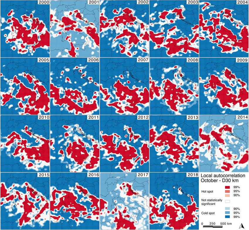
Preliminary spatial local autocorrelation analysis was performed for every month in the 19 years
Preliminary
Preliminaryspatial
spatiallocal
localautocorrelation
autocorrelationanalysis
analysiswas
wasperformed
performedforforevery
everymonth
monthininthe
the19
19years
years
of measurements: in Figure 10, the results for October are shown. Analysis allows to identify the hot
of
ofmeasurements:
measurements: in Figure 10,
Figure 10, the
theresults
resultsfor
forOctober
Octoberareareshown.
shown.Analysis
Analysis allows
allows to to identify
identify the the
hot
and cold spots, that is, a clustering of high- and low-density values. Clustering is localized in the
hot
andand
coldcold spots,
spots, thatthat
is, ais,clustering
a clustering of high-
of high- andand low-density
low-density values.
values. Clustering
Clustering is localized
is localized in
in the
Tyrrhenian Sea and in the sea south of Italy, evidencing particular strong activity along all the
the Tyrrhenian Sea and in the sea south of Italy, evidencing
Tyrrhenian Sea and in the sea south of Italy, evidencing particular particular strong activity along all the
along all the
Tyrrhenian–Italian coastlines; more discontinuous clustering affected even the Provence area and the
Tyrrhenian–Italian
Tyrrhenian–Italiancoastlines;
coastlines;moremorediscontinuous
discontinuousclustering
clusteringaffected
affectedeven
eventhe
theProvence
Provenceareaareaand
andthe
the
northern Adriatic Sea. Smaller clustering areas happened in October 2001, 2014, and 2017. Further
northern Adriatic Sea. Smaller clustering areas happened in October 2001, 2014, and 2017. Further
analysis will be conducted in future studies.
analysis will be conducted in future studies.Remote Sens. 2019, 11, 1601 15 of 20
northern Adriatic Sea. Smaller clustering areas happened in October 2001, 2014, and 2017. Further
analysis will be conducted in future studies.
Remote Sens. 2019, 11, x FOR PEER REVIEW 16 of 21
Figure10.
Figure 10. Local
Local autocorrelation
autocorrelationat ataadistance
distanceof D== 30 km for October in the 2000–2018
ofD 2000–2018 period
period at
at 90%,
90%,
95%,and
95%, and99%
99%confidence
confidencelevels.
levels.
4.
4. Discussion
Discussion
Preliminary
Preliminaryanalysis
analysisof ofthe
thespatial
spatialandandtemporal
temporal high-resolution
high-resolutionstroke strokedatabase
databasefor forthe
theCentral
Central
Mediterranean area in the 2000–2018 period allowed to obtain the first result:
Mediterranean area in the 2000–2018 period allowed to obtain the first result: high variability both high variability bothin
in time and space is a common feature for the distribution of total strokes
time and space is a common feature for the distribution of total strokes both per month and per year both per month and per
year
duringduring the examined
the examined period.
period. SuchSuchhigh high temporal
temporal variability
variability has been
has been found found in Africa,
in Africa, thenthen
in a
in a different
different climatic
climatic context,
context, by by Price
Price andAsfur
and Asfur[52]
[52]whowhostudied
studied aa fifty-year
fifty-year series.
series. Year-by-year
Year-by-year
variability
variabilityseems
seemsto to
prevent
preventidentifying
identifyingany statistically significative
any statistically generalgeneral
significative trend in trend
the data,
in implying
the data,
that there is no evidence of a steady rising or descending number of strokes
implying that there is no evidence of a steady rising or descending number of strokes over time. over time.
Exceptionally
Exceptionally intense activity throughout
intense activity throughoutmost mostofof20182018isisanother
another important.
important. TheThe
yearyear
20182018
has
has
been documented as the fourth warmest year globally from 1880 after, 2016, 2017, and 2015,
been documented as the fourth warmest year globally from 1880 after, 2016, 2017, and 2015,
respectively
respectively [53]. Onthe
[53]. On theEuropean
Europeanscale, scale,August
August 2018
2018 was
was thethe
thirdthird warmest
warmest after
after August
August 20162016
and
and
2017. Some authors agree in finding a positive correlation between increasing temperature and
2017. Some authors agree in finding a positive correlation between increasing temperature and
lightning activity on the global scale [21,26], even if a long-term trend in lightning
lightning activity on the global scale [21,26], even if a long-term trend in lightning activity has still activity has still
not
notemerged
emerged[52].
[52]. As
As mentioned,
mentioned, no no increasing
increasing trend
trend inin the
the last
last 19
19 years
years ofof stroke
strokedetection
detectionhas hasbeen
been
clearly found in the area under study here, where the exceptional numbers found in 2018, the last
year of the series, could be occasional. An explanation of the lack of a linear general trend, apart from
the large variability of the phenomenon itself, may be found in a nonlinear relationship betweenRemote Sens. 2019, 11, 1601 16 of 20
clearly found in the area under study here, where the exceptional numbers found in 2018, the last year
of the series, could be occasional. An explanation of the lack of a linear general trend, apart from the
large variability of the phenomenon itself, may be found in a nonlinear relationship between warming
and cloud electrification and, then, lightning activity [26]. Future measurements may allow to point
out a clear tendency if global warming proceeds at a similar rate.
Spatial analysis, combined with temporal analysis, allowed to outline a more complicated
condition, with some emerging local trends. Preliminary analysis allows to obtain some conclusions,
but further research is needed to confirm and better delineate tendencies.
An interesting result has emerged applying global Moran’s I analysis to stroke data as a new
possible approach to lightning studies. Moran’s I clearly indicates data clustering, as expected for
stroke data. Strong clustering was demonstrated as a common feature for all the considered data series,
both for more populated and for sparser ones. When stroke activity has been at the maximum, in
August 2018 cloud–ground strokes were spread almost all over the studied area, but higher densities
were strongly clustered anyway.
Dedicated analysis was performed in order to find eventual different spatial distribution of strokes
between land, sea, and coastal zones; at the global scale, the proportion between strokes on land and
on the oceans is 10:1 [21]. In the study area, examining the monthly data, this ratio looks to be affected
by the seasonal cycle, coherently with previous studies [16–20]. In fall and winter, strokes are prevalent
on the sea, while in spring and summer, that is, the higher activity period, on land. This results in a
proportion of about 1:1 between land and sea occurrence considering the total amount of strokes in the
whole study period. This behavior could be related to the climatic peculiarity of the Mediterranean
Sea and the regional area in respect to the tropical zone, where two-thirds of global lightning activity is
concentrated [14].
The percentage of strokes on land appears to increase in January, February, April, and May with
respect to that on the sea. Sunlight warms the sea and land surface differently due to the different
thermal properties of the two: higher thermal inertia of the sea mass causes it to warm slower as the
season moves from winter to spring and summer, and causes it to cool slower from the hot to the
cold season. As a consequence, lightning activity being related to updraft velocities [54], lightning
and stroke counts are considerably higher in the second part of spring and in summer than in winter
and late fall; similarly, the progressively higher warming in spring in recent years suggests a possible
relationship with an increasing percentage of lightning on land in spring. Quicker warming on land
may induce higher lightning activity than on the sea. This process may be considerably enhanced by
the orographic effect [34] that may partially explain the high density measured in the central Ligurian
coastline (Figure 1).
Then, even if it is not possible to identify a statistically significant general trend in the data for the
studied period and area, many symptoms of possible change emerged from analysis: the Mann–Kendall
trend test on the monthly series at the cell scale evidences areas with statistically significant increments
of activity along all months except December, which showed very limited activity. At the same time,
areas with decreasing activity were identified.
Increasing local activity may be related to intense precipitative events and flash floods that hit many
coastal areas of Italy and of Provence in France in October and November, which are the transitional
months from the warm to the cold season: the strong contrast between cold-air masses coming from
the north with a still-warm sea induces high convective activity and subsequent lightnings and large
thunderstorms [55]. These local trends are coherent with data regarding the increase in sea-surface
temperatures revealed by Pastor et al. [56], and as underlined by Kotroni and Lagouvardos [9].
Many flash-flood events associated with high lightning activity happened under these conditions:
in Liguria in 2010, 2011, and 2014; in the northern Tyrrhenian coastline in 2012 and 2014; in Corsica in
2014 and 2016; in Sicily in 2011 and 2018; and in coastal Provence in 2015. The possible relationship
with the increasing trend of stroke density in the same areas requires further and more detailed analysis,
but spatial local autocorrelation in October allows to clearly identify clustering in the Tyrrhenian SeaRemote Sens. 2019, 11, 1601 17 of 20
and along the Italian coastlines, from north to south, and the Provence coastline: clustering gives
evidence of concentrated activity in the same areas hit by intense rainfall events and associated flash
floods. If the local increasing trend identified through the Mann–Kendall test is confirmed in the future,
then a possible increase of intense precipitation could happen.
5. Conclusions
Analysis allowed to evidence the behavior of cloud–ground strokes during 19 years of
measurements over the central Mediterranean, stressing particular features both in space and time: a
record of more years will eventually allow to confirm the emerging indications that could be related to
surface warming.
The performed analysis emphasizes the importance of high-resolution stroke detection and the
collection of a long-term series database. Despite the lack of agreement in considering lightning activity
as increasing with rising surface temperatures, the results contribute, at a local scale, to the study of the
relationship with climate change. The Mediterranean is a spatially constrained sea with a composite
relationship between land and sea areas due to the complex physiography of the coastlines. Thus,
it may not be considered as a representative region on a global scale but, for the same reasons, it is
considered as one of the more susceptible areas of change [57]. Although two-thirds of global lightning
originates in tropical regions [14], the results arising from long-term series analysis seem to suggest a
possible relationship with increasing temperatures, despite the lack of a statistically significant general
trend that emerges from preliminary analysis. Considering spatial distribution, some local increasing
trends emerge in areas recently affected by intense precipitation and flash floods, while no relation
seems to affect normal floods.
Global Moran’s I analysis allowed to evidence the strong clustering of stroke activity in the
examined period, and the peculiar features in the yearly series between monthly stroke count and
the respective I value. These results suggest that future investigations on the clustering properties of
strokes through space and time are required.
In general, the use of high temporal- and spatial-resolution data will substantially contribute to
the progress of this research. The next evolution may be supported by analysis of lightning intensity
and clustering features to better investigate possible future trends and the relationship with floods
and, particularly, flash floods with not-negligible morphological effects on the mainland and coastland.
The present research is a first step toward a possible identification of spatial and temporal trends that
would allow to elaborate possible future scenarios of higher activity, which may be related to extreme
events like flash floods: coastal areas could be the ones that are most exposed.
Author Contributions: Conceptualization, G.P.; methodology, G.P.; software, G.P.; validation, G.P., C.D., M.B., and
F.F.; formal analysis, G.P.; investigation, G.P. and M.B.; resources, F.F.; data curation, M.B..; writing—original-draft
preparation, G.P., C.D, M.B., and F.F.; writing—review and editing, G.P., C.D., M.B.; supervision, C.D and F.F.
Funding: This research received no external funding.
Acknowledgments: The authors wish to thank CESI S.p.A for making the SIRF lightning database available.
Conflicts of Interest: The authors declare no conflict of interest.
References
1. Rakov, V.A.; Uman, M.A. Lightning: Physics and Effects; Cambridge University Press: Cambridge, UK, 2003.
2. Yair, Y.; Lynn, B.; Price, C.; Kotroni, V.; Lagouvardos, K.; Morin, E.; Mugnai, A.; Llasat, M.C. Predicting the
potential for lightning activity in Mediterranean storms based on the WRF model dynamic and microphysical
fields. J. Geophys. Res. 2010, 115, 1–13. [CrossRef]
3. Smith, J.A.; Baeck, M.L.; Zhang, Y. Extreme rainfall and flooding from supercell thunderstorms.
J. Hydrometeorol. 2001, 2, 469–489. [CrossRef]
4. Soula, S.; Chauzy, S. Some aspects of the correlation between lightning and rain activities in thunderstorms.
Atmos. Res. 2001, 56, 355–373. [CrossRef]Remote Sens. 2019, 11, 1601 18 of 20
5. Yann, S.; Soula, S.; Sauvageot, H. Lightning and precipitation relationship in coastal thunderstorms. J.
Geophys. Res. Atmos. 2001, 106, 22801–22816. [CrossRef]
6. Barnolas, M.; Atencia, A.; Llasat, M.C.; Rigo, T. Characterization of a Mediterranean flash flood event using
rain gauges, radar, GIS and lightning data. Adv. Geosci. 2008, 17, 35–41. [CrossRef]
7. Price, C.; Yair, Y.; Mugnai, A.; Lagouvardos, K.; Llasat, M.C.; Michaelides, S.; Dayan, U.; Dietrich, S.;
Di Paola, F.; Galanti, E.; et al. Using lightning data to better understand and predict flash floods in the
Mediterranean. Surv. Geophys. 2011, 32, 733. [CrossRef]
8. Liou, Y.-A.; Kar, S.K. Study of cloud-to-ground lightning and precipitation and their seasonal and geographical
characteristics over Taiwan. Atmos. Res. 2010, 95, 115–122. [CrossRef]
9. Kotroni, V.; Lagouvardos, K. Lightning in the Mediterranean and its relation with sea-surface temperature.
Environ. Res. Lett. 2016, 11, 034006. [CrossRef]
10. Li, N.; Wang, Z.; Chen, X.; Austin, G. Studies of General Precipitation Features with TRMM PR Data: An
Extensive Overview. Remote Sens. 2019, 11, 80. [CrossRef]
11. Capozzi, V.; Montopoli, M.; Mazzarella, V.; Marra, A.C.; Roberto, N.; Panegrossi, G.; Dietrich, S.; Budillon, G.
Multi-Variable Classification Approach for the Detection of Lightning Activity Using a Low-Cost and
Portable X Band Radar. Remote Sens. 2018, 10, 1797. [CrossRef]
12. Müller, R.; Haussler, S.; Jerg, M.; Heizenreder, D.A. Novel Approach for the Detection of Developing
Thunderstorm Cells. Remote Sens. 2019, 11, 443. [CrossRef]
13. Ashley, W.S.; Gilson, C.W. A reassessment of US lightning mortality. Bull. Am. Meteorol. Soc. 2009, 90,
1501–1518. [CrossRef]
14. Christian, H.J.; Blakeslee, R.J.; Boccippio, D.J.; Boeck, W.L.; Buechler, D.E.; Driscoll, K.T.; Goodman, S.J.;
Hall, J.M.; Koshak, W.J.; Mach, D.M.; et al. Global frequency and distribution of lightning as observed from
space by the Optical Transient Detector. J. Geophys. Res. Atmos. 2003, 108, ACL-4. [CrossRef]
15. Papagiannaki, K.; Lagouvardos, K.; Kotroni, V. A database of high-impact weather events in Greece: A
descriptive impact analysis for the period 2001–2011. Nat. Hazards Earth Syst. Sci. 2013, 13, 727–736.
[CrossRef]
16. Holt, M.A.; Hardaker, P.J.; McLelland, G.P. A lightning climatology for Europe and the UK, 1990–1999.
Weather 2001, 56, 290–296. [CrossRef]
17. Katsanos, D.K.; Lagouvardos, K.; Kotroni, V.; Argiriou, A.A. The relationship of lightning activity with
microwave brightness temperatures and spaceborne radar reflectivity profiles in the Central and Eastern
Mediterranean. J. Appl. Meteorol. Climatol. 2007, 46, 1901–1912. [CrossRef]
18. Shalev, S.; Saaroni, H.; Izsak, T.; Yair, Y.; Ziv, B. The spatio-temporal distribution of lightning over Israel and
the neighboring area and its relation to regional synoptic systems. Nat. Hazards Earth Syst. Sci. 2011, 11,
2125–2135. [CrossRef]
19. Anderson, G.; Klugmann, D. A European lightning density analysis using 5 years of ATDnet data. Nat.
Hazards Earth Syst. Sci. 2014, 14, 815–829. [CrossRef]
20. Cecil, D.J.; Buechler, D.E.; Blakeslee, R.J. Gridded lightning climatology from TRMM-LIS and OTD: Dataset
description. Atmos. Res. 2014, 135, 404–414. [CrossRef]
21. Price, C. Thunderstorms, Lightning and Climate Change. In Lightning: Principles, Instruments and Applications;
Betz, H.D., Schumann, U., Laroche, P., Eds.; Springer: Dordrecht, The Netherlands, 2009. [CrossRef]
22. Brakenridge, G.R. Global Active Archive of Large Flood Events, Dartmouth Flood Observatory, University
of Colorado. Available online: http://floodobservatory.colorado.edu/Archives/index.html (accessed on 30
March 2019).
23. Acquaotta, F.; Faccini, F.; Fratianni, S.; Paliaga, G.; Sacchini, A.; Vilìmek, V. Increased flash flooding in Genoa
Metropolitan Area: A combination of climate changes and soil consumption? Meteorol. Atmos. Phys. 2018,
1–12. [CrossRef]
24. Acquaotta, F.; Faccini, F.; Fratianni, S.; Paliaga, G.; Sacchini, A. Rainfall intensity in the Genoa Metropolitan
Area (Northern Mediterranean): Secular variations and consequences. Weather 2018. [CrossRef]
25. Price, C.; Rind, D. Possible implications of global climate change on global lightning distributions and
frequencies. J. Geophys. Res. Atmos. 1994, 99, 10823–10831. [CrossRef]
26. Williams, E.R. Lightning and climate: A review. Atmos. Res. 2005, 76, 272–287. [CrossRef]
27. Romps, D.M.; Seeley, J.T.; Vollaro, D.; Molinari, J. Projected increase in lightning strikes in the United States
due to global warming. Science 2014, 346, 851–854. [CrossRef] [PubMed]Remote Sens. 2019, 11, 1601 19 of 20
28. Banerjee, A.; Archibald, A.T.; Maycock, A.C.; Telford, P.; Abraham, N.L.; Yang, X.; Braesicke, P.; Pyle, J.A.
Lightning NOx, a key chemistry–climate interaction: Impacts of future climate change and consequences for
tropospheric oxidising capacity. Atmos. Chem. Phys. 2014, 14, 9871–9881. [CrossRef]
29. Clark, S.K.; Ward, D.S.; Mahowald, N.M. Parameterization-based uncertainty in future lightning flash density.
Geophys. Res. Lett. 2017, 44, 2893–2901. [CrossRef]
30. Finney, D.L.; Doherty, R.M.; Wild, O.; Stevenson, D.S.; MacKenzie, I.A.; Blyth, A.M. A projected decrease in
lightning under climate change. Nat. Clim. Chang. 2018, 8, 210. [CrossRef]
31. Lay, E.H.; Jacobson, A.R.; Holzworth, R.H.; Rodger, C.J.; Dowden, R.L. Local time variation in land/ocean
lightning flash density as measured by the world wide lightning location network. J. Geophys. Res. 2007, 112,
D13111. [CrossRef]
32. Poelman, D.R.; Schulz, W.; Diendorfer, G.; Bernardi, M. The European lightning location system EUCLID–Part
2: Observations. Nat. Hazards Earth Syst. Sci. 2016, 16, 607–616. [CrossRef]
33. Mezuman, K.; Price, C.; Galanti, E. On the spatial and temporal distribution of thunderstorm cells. Environ.
Res. Lett. 2014, 9, 124023. [CrossRef]
34. Kotroni, V.; Lagouvardos, K. Lightning occurrence in relation with elevation, terrain slope, and vegetation
cover in the Mediterranean. J. Geophys. Res. Atmos. 2008, 113, D21. [CrossRef]
35. Kar, S.K.; Liou, Y.-A. Influence of Land Use and Land Cover Change on the Formation of Local Lightning.
Remote Sens. 2019, 11, 407. [CrossRef]
36. Köppen, W. Das Geographische System der Klimate, 1–44; Gebrüder Borntraeger: Berlin, Germany, 1936.
37. Kottek, M.; Grieser, J.; Beck, C.; Rudolf, B.; Rubel, F. World Map of Köppen- Geiger Climate Classification
updated. Meteorol. Z. 2006, 15, 259–263. [CrossRef]
38. Reddaway, J.M.; Bigg, G.R. Climatic change over the Mediterranean and links to the more general atmospheric
circulation. Int. J. Climatol. 1996, 16, 651–661. [CrossRef]
39. Faccini, F.; Luino, F.; Sacchini, A.; Turconi, L.; De Graff, J.V. Geohydrological hazards and urban development
in the Mediterranean area: An example from Genoa (Liguria, Italy). Nat. Hazards Earth Syst. Sci. 2015, 15,
2631–2652. [CrossRef]
40. Faccini, F.; Luino, F.; Paliaga, G.; Sacchini, A.; Turconi, L.; de Jong, C. Role of rainfall intensity and urban
sprawl in the 2014 flash flood in Genoa City, Bisagno catchment (Liguria, Italy). Appl. Geogr. 2018, 98,
224–241. [CrossRef]
41. Faccini, F.; Paliaga, G.; Piana, P.; Sacchini, A.; Watkins, C. The Bisagno stream catchment (Genoa, Italy) and
its major floods: Geomorphic and land use variations in the last three centuries. Geomorphology 2016, 273,
14–27. [CrossRef]
42. Bernardi, M.; Ferrari, D. The Italian lightning detection system (CESISIRF): Main statistical results on the first
five years of collected data and a first evaluation of the improved system behavior due to a major network
upgrade. In Proceedings of the 25th International Conference on Lightning Protection, Rhodes, Greece, 2
September 2000.
43. Bernardi, M.; Ferrari, D. Evaluation of the LLS efficiency effects on the lightning density at ground, using the
Italian lightning detection system SIRF. J. Electrost. 2004, 60, 131–140. [CrossRef]
44. Schulz, W.; Diendorfer, G.; Pedeboy, S.; Poelman, D.R. The European lightning location system EUCLID–Part
1: Performance analysis and validation. Nat. Hazards Earth Syst. Sci. 2016, 16, 595–605. [CrossRef]
45. Tobler, W.R. A computer movie simulating urban growth in the Detroit region. Econ. Geogr. 1970, 46, 234–240.
[CrossRef]
46. Tobler, W.R. On the First Law of Geography: A Reply. Ann. Assoc. Am. Geogr. 2004, 94, 304–310. [CrossRef]
47. Moran, P.A.P. Notes on continuous stochastic phenomena. Biometrika 1950, 37, 17–23. [CrossRef]
48. Tu, J.; Xia, Z.G. Examining spatially varying relationships between land use and water quality using
geographically weighted regression I: Model design and evaluation. Sci. Total. Environ. 2008, 407, 358–378.
[CrossRef] [PubMed]
49. Ord, J.K.; Getis, A. Local Spatial Autocorrelation Statistics: Distributional Issues and an Application. Geogr.
Anal. 1995, 27. [CrossRef]
50. Kendall, M.G.; Gibbons, J.D. Rank Correlation Methods, 5th ed.; Griffin: London, UK, 1990.
51. Hamed, K.H. Exact distribution of the Mann-Kendall trend test statistic for persistent data. J. Hydrol. 2009,
365, 86–94. [CrossRef]You can also read