On the use of self-organizing maps in detecting teleconnections. Part II: temporal aspects
←
→
Page content transcription
If your browser does not render page correctly, please read the page content below
On the use of self-organizing maps in detecting
teleconnections. Part II: temporal aspects
Jan Stryhal ( stryhal@ufa.cas.cz )
Institute of Atmospheric Physics Czech Academy of Sciences: Ustav fyziky atmosfery Akademie ved
Ceske republiky https://orcid.org/0000-0002-4853-4357
Romana Beranová
Institute of Atmospheric Physics Czech Academy of Sciences: Ustav fyziky atmosfery Akademie ved
Ceske republiky
Radan Huth
Institute of Atmospheric Physics Czech Academy of Sciences: Ustav fyziky atmosfery Akademie ved
Ceske republiky
Research Article
Keywords: Atmospheric circulation, modes of variability, circulation types, classification, PCA, trends,
SOMs
Posted Date: August 3rd, 2021
DOI: https://doi.org/10.21203/rs.3.rs-719194/v1
License: This work is licensed under a Creative Commons Attribution 4.0 International License.
Read Full License
Page 1/27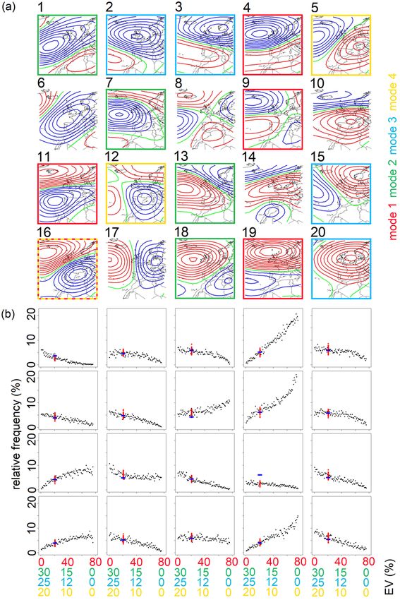
Abstract
Self-organizing maps (SOMs) represent a method widely used to obtain representative states of
atmospheric circulation and link these states to local climate on one hand, and large-scale modes of
circulation variability on the other. In the present Part II of our study, we focus on the temporal aspects of
the link between SOM circulation types (CTs) and main building blocks of spatial-temporal variability
represented by (i) three predefined idealized oscillatory variability modes and (ii) four leading modes of
Euro-Atlantic circulation variability extracted by principal component analysis (PCA). The CTs respond to
various changes in modes, including variations in their strength and preferred phase. However, compared
to these responses, the detected sampling variability inherent to decadal-scale datasets generated from
identical setting of modes is surprisingly high, showing that trends in the frequency of CTs of
approximately ± 30% can occur without any change in the strength and phase of the underlying modes.
This suggests that in order to achieve robust changes in CT frequencies, either an unrealistically large
change in the underlying variability mode, which is inconsistent with reanalysis data, is required, or
simultaneous contributions of two or more modes that superimpose one another are needed.
Consequently, to attribute changes in CTs to variability modes, other methods (e.g., PCA) should be used
in parallel to SOMs to avoid misinterpretations. Since the results obtained for the idealized modes agree
with our findings for real-world circulation, we believe that the rather simplistic idealized modes may be
used in future studies that would extend the research to non-linear aspects of teleconnectivity, including
(but not limited to) non-stationary spatial patterns and non-linear combination of variability modes in
generating synthetic datasets.

1. Introduction
The large-scale atmospheric circulation, its natural variability and changes under climate change have
been extensively studied due to their close links to surface atmospheric elements, especially in mid-
latitudes. Many methods have been used to simplify the wide spatial-temporal variations of atmospheric
circulation, the approaches of circulation classifications and decomposition into modes of circulation
variability being among the favorite ones.

The circulation classifications consist in defining a relatively small number of representative circulation
types (CTs) or recurrent circulation regimes, and classifying fields of a circulation variable with these
types/regimes according to a measure of similarity, which is usually pattern-to-pattern correlation or
Euclidean distance. There are countless algorithms for obtaining a classification, an overview of which
can be found in Huth et al. (2008). This study focuses on one of these algorithms, viz. the self-organizing
maps (SOMs).

The SOMs (Kohonen 2001; Hewitson and Crane 2002; Sheridan and Lee 2011) represent one of the most
popular methods of studying atmospheric circulation. Methodologically, they constitute a neural network
based approach that aims to find a set of states across the circulation data space that together
reasonably approximate all recorded circulation fields. Relative to other wide spread classification

                                                   Page 2/27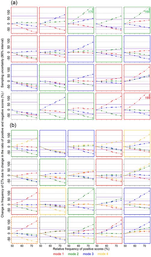
methods, such as the Jenkinson-Collison method or various algorithms of cluster analysis, the SOMs are
not only able to find CTs across the whole spectrum of circulation fields but also sort the CTs into a—
typically two-dimensional—array or “map” that preserves the topological structure of the data space.
Therefore, close (in terms of Euclidean distance; ED) CTs lie in the array relatively closer to each other
while CTs with strong anomalies of opposite sign tend to be “pushed away” from each other into
opposite corners or edges of the array (e.g., Leloup et al. 2007; Reusch et al. 2007; Reusch 2010).
Although studies comparing SOMs with other classification methods (Fleig et al. 2010; Huth 2010; Tveito
2010; Lykoudis et al. 2010; Broderick and Fealy 2015; Trigo et al. 2016; Palm et al. 2017) clearly showed
that different methods turn out to be optimum depending on the application, it has been the SOM that
sparked a new interest in synoptic climatology owing to its novel point of view on circulation variability
(Sheridan and Lee 2011). This interest resulted in a wide range of studies on circulation in outputs of
reanalyses and climate models, links between circulation and various atmospheric and environmental
phenomena, as well as links between synoptic-scale CTs to large-scale teleconnections, bringing new
insights into circulation over Asia (Liu et al. 2016; Gao et al. 2019; Ohba and Sugimoto 2019), Polar
regions (e.g., Schuenemann et al. 2009; Bezeau et al. 2015; Yu et al. 2018), Australia and New Zealand
(e.g., Jiang et al. 2013; Huva et al. 2015; Gibson et al. 2016a,b; Harrington et al. 2016; Theobald et al.
2016,2018), Europe (e.g., Tymvios et al. 2010; Polo et al. 2011), North America (e.g., Newton et al. 2014;
Cassano et al. 2016,2017; Swales et al. 2016; Sugg and Konrad II 2017; Díaz-Esteban and Raga 2018),
South America (Espinoza et al. 2012; Rodríguez-Morata et al. 2018), and southern Africa (e.g., Lennard
and Hegerl 2015; Engelbrecht and Landman 2016; Wolski et al. 2018; Quagraine et al. 2019).

Relative to classifications, modes of variability provide a conceptually different approach to describe
circulation in which individual modes represent main building blocks of spatial-temporal co-variability.
The modes have typically been defined by means of rotated S-mode PCA (SPCA; e.g., Barnston and
Livezey 1987; Huth et al. 2008); see Part I for more information and references on S-mode decomposition.
While in the classification approach, one represents each circulation field by one (most similar) type and
the whole dataset is approximated by a few types and their frequencies, in the case of circulation modes,
each field is represented by a weighted—typically linear—combination of modes and the whole dataset is
approximated by a few modes (first few rotated components) and their explained variances.

The concept of teleconnections, which represent statistical relations between climatic variables at distant
locations (Ångström 1935; Wallace and Gutzler 1981), is closely related to the concept of modes of low-
frequency large-scale variability. Consequently, modes and teleconnections are often considered
synonyms. However, different methods of studying teleconnections and even conceptual perspectives of
teleconnections can be found in literature. Barnston and Livezey (1987) identify SPCA and correlation
maps as the leading methods. In correlation maps of a variable, one obtains temporal correlations
between a base point and all other points across a spatial domain. A subsequent careful selection of
appropriate base points leads to identifying main action centers, or centers of co-variability. Such action
centers that are statistically linked have also been utilized to define various point-based indices, which
can be understood as stand-alone and simplest representations of teleconnections.

                                                   Page 3/27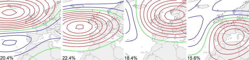
The above mentioned methods of identifying teleconnections have been disputed by some researchers
pointing to their limitations including spatially fixed structure, spatially symmetric opposite phases,
normality, linearity and/or orthogonality imposed on data, and possible extraction of statistical artifacts
rather than physical modes (e.g., Monahan et al. 2001; Chen and Van den Dool 2003; Cassou et al. 2004;
Sheridan and Lee 2012; Hunt et al. 2013). Instead, Cassou et al. (2004) applies cluster analysis to low-
pass filtered North Atlantic–European sea level pressure (SLP) fields produced by National Centers for
Environmental Prediction–National Center for Atmospheric Research (NCEP–NCAR) reanalysis to obtain
four significant climate regimes, the first two of which capture the negative and positive phases of the
North Atlantic Oscillation (NAO; Hurrell et al. 2001), providing a non-linear and non-symmetrical
perspective of the leading teleconnection in the region. To extend this continuum perspective of
teleconnections, Johnson et al. (2008) apply SOMs to Northern Hemisphere SLP data. Leading
teleconnections are then represented by one or more of the CTs in a SOM array and changes in the
teleconnections are assessed by evaluating variations in the occurrence of the respective CTs. Various
teleconnections have been analyzed utilizing this alternative perspective, including El Niño–Southern
Oscillation (e.g., Leloup et al. 2007; Johnson 2013; Ashok et al. 2017), Madden-Julian oscillation
(Chattopadhyay et al. 2013), the Indian Ocean dipole (Tozuka et al. 2008; Verdon-Kidd 2018), the Arctic
oscillation (Dai and Tan 2017), as well as North Pacific (Johnson and Feldstein 2010; Yuan et al. 2015)
and North Atlantic (Johnson et al. 2008; Rousi et al. 2015, 2020) teleconnections.

The two perspectives on teleconnections relying on different decompositions of spatial-temporal
variability are distinct and demand specific interpretation, but also closely linked together and
complementing each other, and applying them in parallel provides potential for new findings. However,
only few studies have compared the approaches from the methodological point of view (Reusch et al.
2005, 2007; Liu et al. 2006; Rousi et al. 2015). In Part I of the study, we analyzed how predefined idealized
modes of variability project on SOM arrays, and whether the two-dimensional SOMs are able to capture
other modes than the leading two modes of variability, as far as the spatial patterns are concerned. In the
present Part II, we focus on the temporal aspects of the link between modes of variability and SOM CTs,
namely on how CT frequency of occurrence depends on data sampling, strength of modes and its
changes, and on the phase of modes. Furthermore, to assess the validity of our findings for real
atmospheric data, results obtained for idealized and real-world variability modes are compared. The
paper is organized as follows: In Sect. 2, we describe the methodology of generating and analyzing the
synthetic datasets and training of SOMs, in Sect. 3.1 we show results for idealized variability modes, in
Sect. 3.2 we focus on Euro-Atlantic variability modes, and in Sect. 4 we provide discussion and
conclusions.

2. Data And Methods
In the paper, two kinds of synthetic data sets are used to test the projection of variability modes on SOMs,
the first constructed using three idealized modes, which are identical to Part I, the other based on modes
calculated by SPCA of daily mean winter 1948–2016 NCEP-NCAR Euro-Atlantic 500 hPa geopotential
height (GPH) fields.
                                                  Page 4/27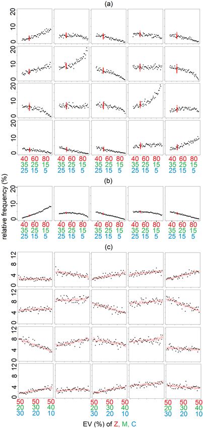
2.1 Synthetic data generated from idealized modes of
variability
The idealized modes express variability in zonal (Z), meridional (M), and circular (C) flow; spatial patterns
of positive phases of the modes (denoted as Z+, M+, C+) are shown in Fig. 1. The modes are defined as
orthogonal so that they mimic modes identified by SPCA. Using the modes, 100 datasets were generated,
each dataset comprising 1,000 circulation fields that consist of 20×20 grid points, each field being a
linear combination of the three modes, where each mode is multiplied by a score. The scores are drawn
from normal distributions, the mean of which is equal to zero and variance equal to the predefined
explained variance (EV) of the particular mode. Note that this process is equivalent to reconstruction of
data from principal components (PCs) obtained by SPCA decomposition, except for randomly generating
the weights instead of obtaining them from the time series of PC scores. One particular combination of
EVs of modes was selected from the variants tested in Part I—“Z50-M30-C20” (each number representing
the EV of the given mode), as this choice gives ample opportunity for modifying the EVs of each mode in
either direction. Additionally, it ensures that a wide range of fields is generated, which in turn means that
all modes are represented among CTs. In the next step, more datasets were generated in which the EV of
the leading mode gradually increases (decreases) at a step of 1 percentage point while variance is
proportionally subtracted from (added to) the remaining two modes. Additionally, several datasets were
generated in which only the scores were altered while EVs of modes remained fixed.

2.2 Synthetic data generated from Euro-Atlantic modes of
variability
The North-Atlantic variability modes were obtained by SPCA decomposition of winter (DJF) 1948–2016
daily mean 500 hPa GPH anomaly fields from the output of the NCEP/NCAR reanalysis (Kalnay et al.
1996). The normalization was carried out separately for each calendar day by subtracting the respective
68-year average, for a spatial domain of 20×20 grid points covering the area of 22.5–70N and 30W–
17.5E (at 2.5° horizontal step). Furthermore, the value at each grid point was weighted by the area that
the grid point represents in order to account for an uneven spatial sampling density. Subsequently, the
covariance matrix was calculated from the data and decomposed by SPCA. The leading four PCs, which
together explain approximately 77% of the total variability, were retained. Rather than analyzing the
output directly, the PCs were first rotated using the Varimax orthogonal rotation (Richman 1986). Rotation
of PCs is recommended in order to remove statistical artifacts that may occur among the modes (Huth
and Beranová 2021). In Fig. 2 the spatial patterns and EVs of the four variability modes are shown.

The obtained modes were then used to generate quasi-realistic daily anomaly patterns in the same
manner as for idealized modes, that is, using the (normalized) rotated loadings as spatial patterns of
modes and variance of the rotated PCs as a parameter for generating time series of scores. First, a total
of 100 data sets (each comprising 1,000 daily patterns) were generated, each having loadings and EVs of
modes fixed to the values we had obtained for rotated PCs, but relaxed time series of scores (see Fig. 3).

                                                   Page 5/27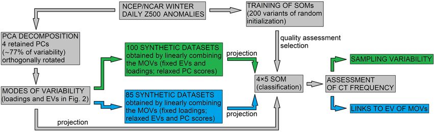
To properly account for the variability explained by non-retained PCs, each daily pattern was further
superimposed by a noise pattern generated randomly such that its spatial autocorrelation approximates
that of the reanalysis anomaly data after the information explained by the four retained PCs was
removed and the total variance explained by the noise patterns in each grid point approximates the
combined variance of non-retained PCs. For simplicity, spatial variations in the autocorrelation were
ignored—its values between neighboring points were set to 0.9. The data were generated serially
uncorrelated, since temporal autocorrelation would not have any effect on any of our intended analyses.

Second, datasets were generated in which the EV of the first mode gradually increases (decreases) at a
step of 0.9 percentage points from 20.4% (its strength in NCEP/NCAR) while variance is subtracted from
(added to) the remaining three modes at a step proportional to their EV in the reanalysis. Therefore, the
EV of the first mode across the 85 generated datasets ranges from 0.6–76.2%. The variance explained by
noise is identical in all kinds of datasets generated from real-world modes (approximately 23%). Third,
several datasets were generated in which only the distribution of scores was altered (shifted toward
positive scores), while EVs of modes remained fixed.

Last, several additional datasets were defined for both idealized and real-world modes, including datasets
that comprise 10,000 instead of 1,000 fields. The motivation behind these auxiliary datasets and their
exact specification is deferred to later in the text.

2.3 Training of SOMs and classification of data
In the next step, all datasets were classified by SOMs, using the “Kohonen” R package (Wehrens and
Buydens 2007; Wehrens and Kruisselbrink 2018). The output of a SOM classification depends on multiple
parameters, including the way how the iterative process is initialized and what is the size (i.e. number of
CTs) and shape (i.e. number of rows and columns of the two-dimensional array of CTs) of the particular
SOM. We considered several sizes of SOM arrays, ranging from 2×3 (rows × columns) to 6×7. Utilizing
results of Part I and additional preliminary analyses, the 4×5 SOM array (20 CTs) was chosen for this
study, since smaller arrays did not include enough types resembling lower-order modes, while larger
arrays tended to have bad topology and/or comprise too many too similar patterns.

The methodology is indicated in Fig. 3 for the Euro-Atlantic modes of variability: First, the reanalysis data
were used to train 200 SOMs that differ only in their random initialization. Second, from these SOMs, one
was selected by evaluating their quantization and topological errors. Third, both reanalysis data and all
generated datasets were projected onto the SOM, by classifying each circulation field with the closest (in
terms of Euclidean distance) CT, and calculating the frequency of occurrence of each CT in each dataset.

To analyse the links between modes and types, the types were further meta-classified by calculating the
correlation between their pattern and the patterns of modes. A type represents the positive (negative)
phase of a mode if the pattern correlation is stronger than a positive (negative) threshold value. The
choice of such threshold is to some extent arbitrary, nevertheless, it needs to reflect the structure of data
(the fewer the modes, the higher the correlations) and parameters of the classification (the fewer the

                                                   Page 6/27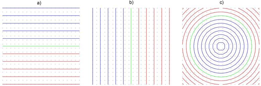
types, the lower the correlations). In general, the value should be higher than 0.7 (R2 ≈ 50%), in order that
one mode contributes to most of its spatial variability. On the other hand, too high a threshold could lead
to some modes (especially, the lower-order ones) being unrepresented. For idealized modes, the value 0.8
seemed to be a good compromise between the two requirements, although it had to be relaxed to 0.75 for
the third-order mode. In the case of real-world modes, which led to more complex data, a lower threshold
(0.7) was chosen.
The idealized modes were analysed in a nearly identical way, except for predefining the modes instead of
extracting them from the reanalysis data and training the SOMs in one of the generated datasets instead
of in the reanalysis data.
Since the processes of quality evaluation of SOMs and selection of other important SOM parameters
were described and discussed in detail in Part I, we refer an interested reader there.
3. Results
3.1 Idealized variability modes
In this section, we describe results for datasets generated from three idealized variability modes. First, the
sampling variability of the frequency of CTs is analyzed; second, the sensitivity of CT frequency to
changes in EV of modes is analyzed; and third, the sensitivity of CT frequency to changes in the phase of
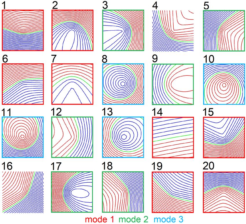
modes is assessed. All results are obtained by projecting generated datasets on a 4×5 SOMs, shown in
Fig. 4, which was trained on one of the 100 Z50-M30-C20 datasets. In the figure, CTs with spatial pattern
similar to one of the modes are highlighted (Fig. 1): eight CTs (clustered in two opposite corners)
resemble the zonal mode, and six (four) CTs closely resemble the meridional (circular) mode. In Part I, we
showed that the third-order mode projects on the 2D SOM arrays rather weakly; here, this is also apparent
from the overall lower pattern correlations for the circular mode. In order that both phases of the mode
are represented, the threshold correlation is set lower (0.75) than for the leading two modes (0.8).
The sensitivity of CT frequencies to random generation of scores of modes (without changing the ratio of
EVs) is first analyzed for datasets comprising 1,000 fields (Fig. 5a; red dots). This size of datasets
approximates the length of a time series of daily fields for one 3-month season and decade (≈ 900 days).
The results should, therefore, be indicative of the rate of sampling uncertainty one needs to consider
when interpreting decadal-scale changes in atmospheric circulation. For this size of datasets, the
sampling variability seems to be rather large: while the relative frequency of CTs varies between about 2%
and 8%, an average sampling variability (expressed as the range of frequencies) is about 3.5 percentage
points. In other words, if one considers a CT occurring 50 times in the datasets on average, such a CT
occurs in individual datasets in about 33–66 instances.
Since the “average” (or, population) frequency of CTs is in reality unknown, a more useful way to express
the variability may consist in looking at dataset-to-dataset differences in the frequency of individual CTs,
Page 7/27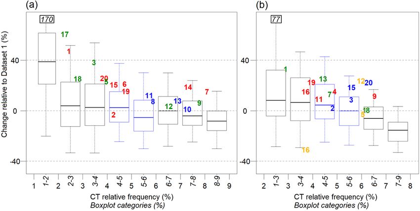
drawing pairs of datasets randomly from the pool of 100 datasets. In Fig. 6a, the boxplots show the rate
of these differences as well as how the differences depend on the relative frequency of CTs. The change
in rare CTs (relative frequency under 2%) appears to be overwhelmingly positive and the interval
containing the 90% of values between the 5th and 95th percentile (hereafter, “90% interval”) is very wide
(approx. -20–170%). On the other hand, the interval is narrowest and most of the differences negative for
the most common CTs (approx. -30–20%). For the two categories between 4–6% (highlighted in blue in
Fig. 6a), which are representative of most CTs due to the tendency of the classification to produce equally
populated clusters, the 90% interval is bounded by approximately ± 30%.

The bias toward positive (negative) trends in small (large) CTs is due to how CT frequency is expressed;
in this case, it does not refer to the population frequency but rather to the frequency in one of the two
randomly generated datasets (“Dataset 1”, or “reference”). The result suggests that when interpreting
differences between classifications, a tendency to positive (negative) trend in CT frequencies of small
(large) CTs may be linked to sampling variability rather than real changes in circulation, e.g., variability
modes. In general, both perspectives of sampling uncertainty indicate that in the case of a decrease or an
increase in CT frequency, especially that which is smaller than about 30%, one should not neglect the
effect of sampling on results. In Fig. 5b, we show (for the first row of CTs only) the same result as in
Fig. 5a, except for larger datasets (n = 10,000). Such an increase in size leads to a marked decrease in
sampling variability in CT frequencies by approximately 70%.

The sensitivity of CT frequencies to gradual changes in the strength of modes is tested in several
experiments. First, we analyse datasets in which the strength of all three modes changes simultaneously
(Fig. 5a, black dots). For a majority of CTs, changes in EV of modes lead to apparent trends in the
frequency of their occurrence, but not for all of them. For example, from the eight “zonal” CTs, #2 and #15
respond only very weakly even if the mode explains nearly all variability. CT #13, which is most similar to
the pattern of the third mode (C), responds very weakly to changes in EV of that mode, and stays quite
frequent even if the mode is nearly turned off. This lack of response of #13 is replicated in another
experiment (Fig. 5c), in which the EV of Z is fixed and EV is gradually subtracted from C and added to M.
In this case, a drop in EV of C by 67% leads to a rather small 25% decrease in frequency. Last but not
least, when EV of Z is fixed, most zonal CTs seemed to have a trend—albeit weak—due to changes in
other modes.

Marked changes in frequency of CTs are apparent only for rather extreme changes in EVs, which are
unlikely to occur in reality, at least for leading modes, as will be documented later for reanalysis data. To
generalize the results, and to assess the rate of changes in CT frequency to rather strong, but feasible,
changes in EV of modes, we analyze the change in CT frequency equivalent to strengthening of modes by
20%. To circumvent the large sampling variability, the change in frequency is calculated utilizing the large
datasets (shown in Fig. 5b) and is indicated in Fig. 6a (colored numbers). In the figure, the position of all
CTs meta-classified with a mode (see Fig. 4) corresponds to their relative frequency (horizontal axis) and
the change relative to this frequency due to strengthening of the mode the particular CT represents by
20% (e.g., the response in “Z” CTs is calculated by comparing Z60-M25-C15 to Z50-M30-C20). Of the 18
                                                  Page 8/27
CTs associated with a mode, only one CT (#17) has a response outside the 90% interval of sampling
variability. We also carried out an identical analysis, except for weakening of the modes (not shown). In
this case, four CTs (#1, #8, #17, and #20) lied outside the interval. However, in nearly all cases, there is an
agreement in the sign of the change (that is, all zonal CTs become less frequent if variance is subtracted
from the zonal mode, and vice versa). This is what differentiates the response to changes in EV from
sampling variability, for which the number of positive and negative changes in CTs associated with a
mode tends to be approximately equal (not shown).
Last, we analyze the sensitivity of CT frequency to changes in the phase of modes. To this end, three sets
of large datasets (10,000 fields; one set per mode) are generated in which the ratio of positive and
negative scores of one mode is shifted from the original 50:50 distribution in favor of positive scores (the
remaining two modes being unchanged). We focus in detail on two specific examples (60:40, i.e.,
increase in frequency of positive scores by 20%, and 2:1); several other cases are also presented in
Fig. 7a. Shifting a mode toward one phase seems to have a considerably more robust response in the
frequency of CTs associated with the mode, compared to simply making the mode stronger: When
changing the ratio to 60:40, the response in 72% of CTs can be distinguished from sampling variability,
while there are no cases in which a CT would have a robust response to the same change in a mode it is
not associated with. When the ratio is further increased to 2:1, all CTs have a robust response to the
change in the mode they represent. However, in this case, five (28%) CTs respond also to the shift in one
of the modes with which they are not associated. For example, #2, associated with the zonal mode
(pattern correlation of -0.84, that is, it represents the mode in its negative phase) becomes 26% less
frequent if the scores of Z are shifted to 60:40, and even 32% more frequent if the scores of C are shifted
instead, neither of the two values being outside the 90% interval of sampling variability of this CT. If the
ratio of scores is further increased to 2:1, the CT has a robust response to changes in both modes (-41%
for Z, + 55% for C). It is not clear why the response is stronger to changes in a mode with which the CT is
less associated (r < 0.5), but it shows that even if one specific kind of change in modes can be isolated,
attributing changes in CTs to particular modes is far from straightforward.
3.2 Euro-Atlantic variability modes
In this section, experiments carried out on datasets generated from variability modes extracted from
NCEP/NCAR reanalysis data are described and discussed. The goal of the study is to assess to what
extent the findings obtained for idealized modes of variability, shown above as well as in Part I of the
study, are applicable to real atmospheric circulation variability. Therefore, to ensure comparability the
methodologies of analyzing idealized and real-world modes are as similar as possible, including the
choice of the grid (20×20 points) and SOM array (4×5 CTs). Compared to idealized data, the generated
datasets are considerably more complex in this case. Four variability modes, together explaining
approximately 77% of variability in winter daily 500 hPa GPH fields were retained and rotated. After
rotation, the spatial patterns (Fig. 2) of the leading three modes resemble the regional structure of NAO,
the East-Atlantic pattern, and the Eurasian pattern type 2, in turn (Barnston and Livezey 1987; Beranová
nad Huth 2008). The weakest mode having one variability center in the Mediterranean region does not
Page 9/27resemble any mode identified in other studies. We refer to the modes by their generic names (mode 1,
mode 2, etc.) in the text, since—except for NAO—we believe that the lower-order variability modes are not
generally known and/or are known under various names.
In Fig. 8a, the SOM of reanalysis data is shown. Fifteen (out of twenty) CTs are associated with modes,
and each mode is associated with between 3–5 CTs. Each of these CTs is associated with one mode,
except for #16 that is strongly correlated both with mode 1 and 4 (|r| ≈ 0.85); it is therefore meta-
classified with two modes. The CT relative frequency in the reanalysis is indicated in Fig. 8b. The
occurrences of most CTs in the reanalysis (blue hyphen) and in datasets generated from the real-world
modes (red dots) are in agreement. The generated data markedly underestimate (overestimate) the
occurrence of CTs #14 (#8), both of which are correlated with the modes only relatively weakly. Therefore,
they are not associated with any of the modes, and as such they are not considered in the further
analysis.
The sampling variability of CT frequencies in datasets with fixed EV of modes and relaxed component
scores and the sensitivity of CT frequencies to gradual changes in the strength of modes are indicated in
Fig. 8b by red and black dots, respectively. The sampling variability averaged over the 15 meta-classified
CTs is nearly identical to that of idealized modes, that is, 3.5 percentage points; therefore, a CT occurring
50 times in the datasets on average appears in individual datasets in approximately 33–66 instances.
The sensitivity of CT frequencies to changes in EVs of real-world modes is also very similar to the
idealized modes. Evidently, some CTs do not respond to changes in EV of associated modes at all (esp.
#18, associated with mode 2) or respond only in a narrow band of the tested EV spectrum (all CTs
associated with mode 4). The response in CTs associated with a mode is in most cases directly
proportional to the change in EV of the mode; nevertheless, it seems to be relatively weak compared to
sampling variability, unless unrealistically large changes in EVs are considered. In the reanalysis, the
change in EV of individual modes between consecutive periods of 1,000 days rarely (never) exceeds 20%
(25%), or four (five) percentage points. In other words, most of the range of EVs tested here and shown in
Fig. 8b is theoretical and only cases close to the EVs observed in the reanalysis are of further practical
interest.
In Fig. 6b, we show the change in relative frequency of CTs caused by strengthening of the mode (with
which the particular CT is associated) by 20% and compare it to sampling variability. Identically to the
idealized modes above, the variability is expressed as a relative change in frequency between multiple
pairs of randomly selected datasets and shown by boxplots for several categories of CT frequencies. The
results are very similar to those for the idealized modes; the position and the width of the 90% interval of
sampling variability both depend on CT frequency in the reference dataset (DS1), the differences being
rather large and overwhelmingly positive in small CTs and somewhat smaller and largely negative in
large CTs. The variability in the CTs close to the median frequency (4–6%, in blue boxplots in Fig. 6b) is
close to the ± 30% found for the idealized modes above. Of the 15 CTs, none has a response to
strengthening (Fig. 6b, numbers) or weakening (not shown) of “its” mode by 20% that would lie outside of
Page 10/27the 90% interval of its own sampling variability (Note that these intervals differ from those shown in the
boxplots, which do not discriminate between CTs).
Except for the weakest mode, there is an agreement in the sign of changes of EV of modes and
frequencies of associated CTs. Namely #16, associated with both mode 1 and 4, becomes markedly less
frequent when mode 4 becomes stronger, due to its response to the simultaneous weakening of mode 1.
This illustrates a drawback of interpreting changes in CT frequency in terms of changes in strength of
teleconnections (i.e., EV of modes)—most of CTs have relatively high correlations with at least one
additional mode, and they respond to changes in both modes. The other CTs with the weakest response
to strengthening of “their” mode (#2, #3, #5, #18) all have relatively high pattern correlation with mode 1
(|r| > 0.5), and the positive trend due to “their” mode is mitigated, or even overturned due to change in
mode 1. The response in CTs would likely further change if the variance added to one mode was
subtracted from the remaining modes in a different way than how it was done here (not tested for real-
world modes). Since the agreement in the sign of change of frequencies of associated CTs seems to be
the only way to distinguish sampling variability from a response to change in EV, attributing changes in
CT frequencies does not seem to be a reliable approach, at least for lower-order modes.
The sensitivity of CT frequency to changes in the phase of modes is shown in Fig. 7b. The response of
CT frequencies to changes in the ratio of positive and negative scores is calculated independently for
each mode (the ratio for the remaining three modes being fixed at approximately 50:50) utilizing datasets
of 10,000 fields to minimize the effects of sampling. The most extreme ratio of scores in the reanalysis
data (observed over six consecutive periods of 1,000 fields) is approximately 58:42; the most extreme
change in the percentage of scores of one sign between two consecutive periods is approximately ± 10
percentage points, or ± 20% (not shown). Various ratios are shown in Fig. 7b; nevertheless, the change
from 50:50 to 55:45 (60:40) is discussed in detail, as it best represents the common (most extreme)
cases observed in the reanalysis. The shift to 55:45 (modes in their strong positive phase) does not lead
to a change in CT frequency in any of the associated CTs robust enough to be discernable from sampling
variability. The shift to 60:40 (modes in their extreme positive phase) leads to a robust change in 50% of
CTs, and with the exception of #2, CTs have a robust response only to their associated mode. In the
theoretical ratio 2:1 (not observed in reanalysis at decadal scale), most CTs respond to at least two
different modes. The results document that even though the sensitivity of CT frequency to shifts in the
phase of modes is greatest for the associated mode, all CTs respond to more (in some cases even all
four, for example #2) modes. This tendency was also apparent for idealized modes, but here it is more
pronounced, likely because of much more equally distributed variance among the real-world modes
and/or more modes. Consequently, there are fewer CTs that reflect a single mode because there are fewer
cases in the data space in which all but one mode are close to their neutral phase.
4. Discussion And Conclusions
In Part II of our study, we focused on the temporal aspect of the link between modes of variability, or
functions of spatial-temporal co-variability of atmospheric circulation fields, and CTs defined by SOMs,
Page 11/27complementing Part I that focused on the spatial aspect of the link. To assess the validity of results for
real-world data, the study was expanded by including reanalysis data, namely the variability modes
extracted from daily GPH fields over the Euro-Atlantic region. The results obtained for idealized and real-
world variability modes were compared and the overall very good agreement suggests that
methodological findings obtained for idealized modes are valid for more complex atmospheric variability,
in spite of notable differences in the number, complexity of spatial patterns and distribution of explained
variances of the modes, and inclusion of noise in datasets based on real-world modes. Although little
effect of adding noise to data on conclusions was expected due to similar findings by Reusch et al.
(2005) and Liu et al. (2006), its confirmation—together with little dependence of results on the kind of
utilized modes—suggests that the idealized modes, which are easy to interpret and work with, could be
used in the next step expanding the research to more complex studies including non-linear definition
and/or combination of modes.
The choices of how synthetic datasets were generated and which methods were used to analyze them
were discussed in detail in Part I. The generation of datasets by linearly combining the underlying modes
is very straightforward, as it reverses the way how modes are typically obtained (by PCA decomposition).
It differs from previous studies that used synthetic data (Reusch et al. 2005; Liu et al. 2006), which in
most cases generated fields directly from anomaly patterns, which resulted in a few well separated
clusters. Such a definition of data is very natural if one wants to assess the ability of a method to classify
data. However, such data fail to mimic the continuous nature of atmospheric circulation fields. Given the
fact that SOMs can be used both for classification and data exploratory projection, unlike SPCA, which
does not provide a classification on its own, we are confident that our data are more suitable for
methodological studies as they make it possible that each method shows its strengths. The data also
allow for different perspectives of teleconnections, that is, preferred quasi-stationary states (Risbey et al.
2015) versus leading components of co-variability, to be investigated in parallel. Regrettably, the different
approach we generate data and the focus of previous studies on the spatial domain disables comparison
of results.
The utilization of synthetic datasets enabled us to investigate how various changes in underlying modes
affect the occurrence of CTs and, more importantly, to isolate the effects of these changes from one
another. Furthermore, by generating multiple datasets that differ only in random generation of scores, or
intensities, of modes, we quantified the sampling uncertainty typical for decadal-scale daily circulation
fields. To our knowledge, modes of variability have not yet been utilized to this end, and we believe that
this methodology could be extended in the future and used to evaluate the expectable variability in
atmospheric circulation in general under the assumptions of stable versus changing variability modes.
Here, the sampling variability of CT frequencies obtained solely by the random generation of scores was
remarkably high, and not only the range of obtained frequencies of CTs but also a narrower 90% interval
in most cases exceeded the signal observed for changes in the strength (variance) or phase of modes of
the rate observed in the reanalysis. Based on our results, we estimate that decadal-scale changes in CT
frequency smaller than approximately ± 30% can occur without any changes in the strength and phase of
any of the underlying variability modes, including their spatial structure. Consequently, future studies
Page 12/27attempting to link changes in CTs to teleconnections should consider sampling uncertainty. Nevertheless,
we stress that the exact value presented here depends on many factors, some of which were tested here
(e.g., frequency of CTs) and some of which not (e.g., parameters of the classification, such as the number
of CTs).
The signal of specific alterations of an underlying mode consists in a concordant behaviour of most CTs
associated with the mode. Here, the association was done by comparing the spatial similarity between
the patterns of CTs and modes, following Yuan et al. (2015) and Rousi et al. (2020); we did not analyze
the similarity in the temporal domain. Despite a variable rate of change, the sign of change in a set of CTs
associated with a mode typically agrees with the sign of change in EV of the mode, and the two subsets
resembling the positive and negative phases respond rather predictably to a shift of the mode toward one
of its phases. However, a change in the frequency of a CT well outside of the sampling variability
typically requires an unrealistically large change in the underlying mode.. This suggests that very strong
changes in CT frequencies, documented for example in studies on Euro-Atlantic decadal-scale circulation
variability (e.g., Johnson et al. 2008), are likely due to superimposed changes in underlying modes, that is,
simultaneous strengthening and shift toward one phase of one mode and/or simultaneous changes in
more than one mode. This is in agreement with the results of Jiang et al. (2013), who additionally point to
the fact that the simultaneously acting factors can, on the other hand, counter-effect one another, making
attribution problematic. Here, this behaviour was most apparent for the weakest mode, the contribution of
which was in some cases overturned by changes in stronger modes.
Although we are aware that the conclusions relate much more closely to the concept of teleconnections
as stationary linear oscillatory features, we believe that they should also be considered in studies that
understand teleconnections in the continuum perspective of physical states, especially since PCA is used
to delimit teleconnections within the SOM phase space.
Declarations
Acknowledgements
This research was supported by the Czech Science Foundation, project 17-07043S. We acknowledge the
work of all authors of the Kohonen and MASS R packages, without which this study would not have been
possible. NCEP/NCAR reanalysis data were provided by the NOAA/OAR/ESRL PSL, Boulder, Colorado,
USA. We thank Dr. Martin Dubrovský for help with generating data.
Funding
This research was supported by the Czech Science Foundation, project 17-07043S
Conflicts of interest/Competing interests
The authors declare no conflict of interest
Page 13/27Availability of data and material (data transparency)
The NCEP/NCAR data can be accessed via https://psl.noaa.gov/. The predefined modes of variability can
be accessed at dx.doi.org/10.6084/m9.figshare.13288889. The generated datasets were not uploaded
due to capacity constraints but will be provided upon request
Code availability (software application or custom code)
Not applicable
Authors' contributions
Not applicable
Additional declarations for articles in life science journals that report the results of studies involving
humans and/or animals
Not applicable
Ethics approval
Not applicable
Consent to participate
Not applicable
Consent for publication
Not applicable
References
Ångström A (1935) Teleconnections of climatic changes in present time. Geografiska Annaler 17:242–
258. doi:10.1080/20014422.1935.11880600
Ashok K, Shamal M, Sahai AK, Swapna P (2017) Nonlinearities in the evolutional distinctions between El
Niño and La Niña types. J Geophys Res Oceans 122:9649–9662. doi:10.1002/2017JC013129
Barnston AG, Livezey RE (1987) Classification, seasonality and persistence of low-frequency atmospheric
circulation patterns. Mon Wea Rev 115:1083–1126. doi:10.1175/1520-
0493(1987)1152.0.CO;2
Beranová R, Huth R (2008): Time variations of the effects of circulation variability modes on European
temperature and precipitation in winter. Int J Climatol 28:139–158. doi:10.1002/joc.1516
Page 14/27Bezeau P, Gascon G (2015) Variability in summer anticyclonic circulation over the Canadian Arctic
Archipelago and west Greenland in the late 20th/early 21st centuries and its effect on glacier mass
balance. Int J Climatol 35:540–557. doi:10.1002/joc.4000
Broderick C, Fealy R (2015) An analysis of the synoptic and climatological applicability of circulation type
classifications for Ireland. Int J Climatol 35:481–505. doi:10.1002/joc.3996
Cassano EN, Cassano JJ, Seefeldt MW, Gutowski WJ, Glisan JM (2017) Synoptic conditions during
summertime temperature extremes in Alaska. Int J Climatol 37:3694–3713. doi:10.1002/joc.4949
Cassano JJ, Cassano EN, Seefeldt MW, Gutowski WJ, Glisan JM (2016) Synoptic conditions during
wintertime temperature extremes in Alaska. J Geophys Res Atmos 121:3241–3262.
doi:10.1002/2015JD024404
Cassou C, Terray L, Hurrell JW, Deser C (2004) North Atlantic winter climate regimes: spatial asymmetry,
stationarity with time, and oceanic forcing. J Climate 17:1055–1068. doi:10.1175/1520-
0442(2004)0172.0.CO;2
Chattopadhyay R, Vintzileos A, Zhang C (2013) A description of the Madden–Julian Oscillation based on
a self-organizing map. J Climate 26:1716–1732. doi:10.1175/JCLI-D-12-00123.1
Chen WY, Van den Dool H (2003) Sensitivity of teleconnection patterns to the sign of their primary action
center. Mon Wea Rev 131:2885–2899. doi:10.1175/1520-0493(2003)1312.0.CO;2
Dai P, Tan B (2017) The nature of the Arctic oscillation and diversity of the extreme surface weather
anomalies it generates. J Climate 30:5563–5584. doi:10.1175/JCLI-D-16-0467.1
Díaz‐Esteban Y, Raga GB (2018) Weather regimes associated with summer rainfall variability over
southern Mexico. Int J Climatol 38:169–186. doi:10.1002/joc.5168
Engelbrecht CJ, Landman WA (2016) Interannual variability of seasonal rainfall over the Cape south
coast of South Africa and synoptic type association. Climate Dyn 47:295–313. doi:10.1007/s00382-015-
2836-2
Espinoza JC, Lengaigne M, Ronchail J, Janicot S (2012) Large-scale circulation patterns and related
rainfall in the Amazon Basin: a neuronal networks approach. Climate Dyn 38:121–140.
doi:10.1007/s00382-011-1010-8
Fleig AK, Tallaksen LM, Hisdal H, Stahl K, Hannah DM (2010) Intercomparison of weather and circulation
type classifications for hydrological drought development. Phys Chem Earth 35:507–515.
doi:10.1016/j.pce.2009.11.005
Gao M, Yang Y, Shi H, Gao Z (2019) SOM-based synoptic analysis of atmospheric circulation patterns
and temperature anomalies in China. Atmos Res 220:46–56. doi:10.1016/j.atmosres.2019.01.005
Page 15/27Gibson PB, Perkins‐Kirkpatrick SE, Renwick JA (2016a) Projected changes in synoptic weather patterns
over New Zealand examined through self‐organizing maps. Int J Climatol 36:3934–3948.
doi:10.1002/joc.4604
Gibson PB, Uotila P, Perkins-Kirkpatrick SE, Alexander LV, Pitman AJ (2016b) Evaluating synoptic systems
in the CMIP5 climate models over the Australian region. Climate Dyn 47:2235–2251. doi:10.1007/s0038
2-015-2961-y
Harrington LJ, Gibson PB, Dean SM, Mitchell D, Rosier SM, Frame DJ (2016) Investigating event‐specific
drought attribution using self‐organizing maps. J Geophys Res Atmos 121:766–780.
doi:10.1002/2016JD025602
Hewitson BC, Crane RG (2002) Self-organizing maps: applications to synoptic climatology. Climate Res
22:13–26. doi:10.3354/cr022013
Hunt FK, Hirschi JJ-M, Sinha B, Oliver K, Wells N (2013) Combining point correlation maps with self-
organising maps to compare observed and simulated atmospheric teleconnection patterns. Tellus A
65:20822. doi:10.3402/tellusa.v65i0.20822
Hurrell JW, Kushnir Y, Visbeck M (2001): The North Atlantic Oscillation. Science 291: 603–605.
doi:10.1126/science.1058761
Huth R (2010) Synoptic-climatological applicability of circulation classifications from the COST733
collection: First results. Phys Chem Earth 35:388–394. doi:10.1016/j.pce.2009.11.013
Huth R, Beck C, Philipp A, Demuzere M, Ustrnul Z, Cahynová M, Kyselý J, Tveito OE (2008) Classifications
of atmospheric circulation patterns. Ann N Y Acad Sci 1146:105–152. doi:10.1196/annals.1446.019
Huth R, Beranová R (2021) How to recognize a true mode of atmospheric circulation variability. Earth
Space Sci. 8:e2020EA001275. doi:10.1029/2020EA001275
Huva R, Dargaville R, Rayner P (2015) The impact of filtering self‐organizing maps: a case study with
Australian pressure and rainfall. Int J Climatol 35:624–633. doi:10.1002/joc.4008
Jiang N, Griffiths G, Lorrey A (2013) Influence of large‐scale climate modes on daily synoptic weather
types over New Zealand. Int J Climatol 33:499–519. doi:10.1002/joc.3443
Johnson NC (2013) How many ENSO flavors can we distinguish? J Climate 26:4816–4827.
doi:10.1175/JCLI-D-12-00649.1
Johnson NC, Feldstein SB (2010) The continuum of North Pacific sea level pressure patterns:
Intraseasonal, interannual, and interdecadal variability. J Climate 23:851–867.
doi:10.1175/2009JCLI3099.1
Page 16/27Johnson NC, Feldstein SB, Tremblay B (2008) The continuum of Northern Hemisphere teleconnection
patterns and a description of the NAO shift with the use of self-organizing maps. J Climate 21:6354–
6371. doi:10.1175/2008JCLI2380.1
Kalnay E et al. (1996) The NCEP/NCAR 40-Year Reanalysis Project. Bull Amer Meteor Soc 77:437–470.
doi:10.1175/1520-0477(1996)077,0437:TNYRP.2.0.CO;2
Kohonen T (2001) Self-Organizing Maps. Springer, New York
Leloup JA, Lachkar Z, Boulanger JP, Thiria S (2007) Detecting decadal changes in ENSO using neural
networks. Climate Dyn 28:147–162. doi:10.1007/s00382-006-0173-1
Lennard C, Hegerl G (2015) Relating changes in synoptic circulation to the surface rainfall response using
self-organising maps. Climate Dyn 44:861–879. doi:10.1007/s00382-014-2169-6
Liu W, Wang L, Chen D, Tu K, Ruan C, Hu Z (2016) Large-scale circulation classification and its links to
observed precipitation in the eastern and central Tibetan Plateau. Climate Dyn 46:3481–3497.
doi:10.1007/s00382-015-2782-z
Liu Y, Weisberg RH, Mooers CNK (2006) Performance evaluation of the self-organizing map for feature
extraction. J Geophys Res Oceans 111:C05018. doi:10.1029/2005JC003117
Lykoudis SP, Kostopoulou E, Argiriou AA (2010) Stable isotopic signature of precipitation under various
synoptic classifications. Phys Chem Earth 35:530–535. doi:10.1016/j.pce.2009.09.002
Monahan AH, Pandolfo L, Fyfe JC (2001) The preferred structure of variability of the northern hemisphere
atmospheric circulation. Geophys Res Lett 28:1019–1022. doi:10.1029/2000GL012069
Newton BW, Prowse TD, Bonsal BR (2014) Evaluating the distribution of water resources in western
Canada using synoptic climatology and selected teleconnections. Part 1: winter season. Hydrol Process
28:4219–4234. doi:10.1002/hyp.10233
Ohba M, Sugimoto S (2019) Differences in climate change impacts between weather patterns: possible
effects on spatial heterogeneous changes in future extreme rainfall. Climate Dyn 52:4177–4191.
doi:10.1007/s00382-018-4374-1
Palm V, Sepp M, Truu J, Ward RD, Leito A (2017) The effect of atmospheric circulation on spring arrival of
short- and long-distance migratory bird species in Estonia. Boreal Env Res 22:97–114.
doi:10.3176/eco.2011.2.03
Polo I, Ullmann A, Roucou P, Fontaine B (2011) Weather regimes in the Euro-Atlantic and Mediterranean
sector, and relationship with West African rainfall over the 1989–2008 period from a self-organizing
maps approach. J Climate 24:3423–3432. doi:10.1175/2011JCLI3622.1
Page 17/27Quagraine KA, Hewitson B, Jack C, Pinto I, Lennard C (2019) A methodological approach to assess the co-
behavior of climate processes over southern Africa. J Climate 32:2483–2495. doi:10.1175/JCLI-D-18-
0689.1
Reusch DB, Alley RB, Hewitson BC (2005) Relative performance of self-organizing maps and principal
component analysis in pattern extraction from synthetic climatological data. Polar Geogr 29:188–212.
doi:10.1080/789610199
Reusch DB, Alley RB, Hewitson BC (2007) North Atlantic climate variability from a self‐organizing map
perspective, J Geophys Res 112:D02104. doi:10.1029/2006JD007460
Reusch DB (2010) Nonlinear climatology and paleoclimatology: capturing patterns of variability and
change with self-organizing maps. Phys Chem Earth 35:329–340. doi:10.1016/j.pce.2009.09.001
Richman B (1986) Rotation of principal components. J Climatol 6:293–335.
doi:10.1002/joc.3370060305
Risbey JS, O’Kane TJ, Monselesan DP, Franzke C, Horenko I (2015) Metastability of Northern Hemisphere
teleconnection modes. J Atmos Sci 72:35–54. doi:10.1175/JAS-D-14-0020.1
Rodríguez-Morata C, Ballesteros-Canovas JA, Rohrer M, Espinoza JC, Beniston M, Stoffel M (2018)
Linking atmospheric circulation patterns with hydro-geomorphic disasters in Peru. Int J Climatol 38:
3388–3404. doi:10.1002/joc.5507
Rousi E, Anagnostopoulou C, Tolika K, Maheras P (2015) Representing teleconnection patterns over
Europe: A comparison of SOM and PCA methods. Atmos Res 152:123–137.
doi:10.1016/j.atmosres.2013.11.010
Rousi E, Rust HW, Ulbrich U, Anagnostopoulou C (2020) Implications of winter NAO flavors on present and
future European climate. Climate 8:13. doi:10.3390/cli8010013
Schuenemann KC, Cassano JJ, Finnis J (2009) Synoptic forcing of precipitation over Greenland:
climatology for 1961–99. J Hydrometeor 10:60–78. doi:10.1175/2008JHM1014.1
Sheridan SC, Lee CC (2011) The self-organizing map in synoptic climatological research. Prog Phys
Geogr 35:109–119. doi:10.1177/0309133310397582
Sheridan SC, Lee CC (2012) Synoptic climatology and the analysis of atmospheric teleconnections. Prog
Phys Geogr 36:548–557. doi:10.1177/0309133312447935
Sugg JW, Konrad II CE (2017) Relating warm season hydroclimatic variability in the southern
Appalachians to synoptic weather patterns using self-organizing maps. Clim Res 74:145–160.
doi:10.3354/cr01493
Page 18/27Swales D, Alexander M, Hughes M (2016) Examining moisture pathways and extreme precipitation in the
U.S. intermountain west using self-organizing maps. Geophys Res Lett 43:1727–1735.
doi:10.1002/2015GL067478
Theobald A, McGowan H, Speirs J (2016) Trends in synoptic circulation and precipitation in the Snowy
Mountains region, Australia, in the period 1958–2012. Atmos Res 169:434–448.
doi:10.1016/j.atmosres.2015.05.007
Theobald A, McGowan H, Speirs J (2018) Teleconnection influence of precipitation‐bearing synoptic
types over the Snowy Mountains region of south‐east Australia. Int J Climatol 38:2743–2759.
doi:10.1002/joc.5457
Tozuka T, Luo J-J, Masson S, Yamagata T (2008) Tropical Indian Ocean variability revealed by self-
organizing maps. Climate Dyn 31:333–343. doi:10.1007/s00382-007-0356-4
Trigo RM, Sousa PM, Pereira MG, Rasilla D, Gouveia CM (2016) Modelling wildfire activity in Iberia with
different atmospheric circulation weather types. Int J Climatol 36:2761–2778. doi:10.1002/joc.3749
Tveito OE (2010) An assessment of circulation type classifications for precipitation distribution in
Norway. Phys Chem Earth 35:395–402. doi:10.1016/j.pce.2010.03.044
Tymvios F, Savvidou K, Michaelides SC (2010) Association of geopotential height patterns with heavy
rainfall events in Cyprus. Adv Geosci 23:73–78. doi:10.5194/adgeo-23-73-2010
Verdon-Kidd DC (2018) On the classification of different flavours of Indian Ocean dipole
events. Int J Climatol 38:4924–4937. doi:10.1002/joc.5707
Wallace JM, Gutzler DS (1981) Teleconnections in the geopotential height field during the Northern
Hemisphere winter. Mon Wea Rev 109:784–812. doi:10.1175/1520-
0493(1981)1092.0.CO;2
Wehrens R, Buydens L (2007) Self- and super-organizing maps in R: the Kohonen package. J Stat Softw
21:1–19. doi:10.18637/jss.v021.i05
Wehrens R, Kruisselbrink J (2018) Flexible self-organizing maps in kohonen 3.0. J Stat Softw 87:1–18.
doi:10.18637/jss.v087.i07
Wolski P, Jack C, Tadross M, van Aardenne L, Lennard C (2018) Interannual rainfall variability and SOM-
based circulation classification. Climate Dyn 50:479–492. doi:10.1007/s00382-017-3621-1
Yu L, Zhong S, Zhou M, Sun B, Lenschow DH (2018) Antarctic summer sea ice trend in the context of
high-latitude atmospheric circulation changes. J Climate 31:3909–3920. doi:10.1175/JCLI-D-17-0739.1
Page 19/27You can also read