Technical note: Water table mapping accounting for river-aquifer connectivity and human pressure
←
→
Page content transcription
If your browser does not render page correctly, please read the page content below
Technical note: Water table mapping accounting for river-aquifer
     connectivity and human pressure
     Maillot Mathias1-2 , Nicolas Flipo1 , Agnès Rivière1 , Nicolas Desassis1 , Didier Renard1 , Patrick Goblet1 ,
     and Marc Vincent2
     1
         Geosciences Department, MINES ParisTech, PSL University, Fontainebleau, France
     2
         EPTB Seine Grands Lacs, Paris, France
     Correspondence: Maillot Mathias (mathias.maillot@mines-paristech.fr), Nicolas Flipo (nicolas.flipo@mines-paristech.fr)

     Abstract. A water table mapping method that accounts for surface water-groundwater (SW-GW) connectivity and human
     pressure, such as pumping and underground structures occurrence, has been elaborated and tested in the heavily urbanized
     Parisian area. The method developed here consists in two steps. First, hard data (hydraulic head) and soft data (dry wells)
     are used as conditioning points for the estimation of the SW-GW connection status. A disconnection criteria of 0.75 m is
5    adjusted on observed unsaturated zone depth (UZD). It is a default value in areas where such data are missing. The second step
     consists in the final mapping of water table. Given the knowledge of the disconnection criteria, the final map is achieved with
     an ordinary kriging of the UZD that integrates the surface water elevation as a nil unsaturated zone where it is relevant. The
     methodology is demonstrated on two datasets of UZD observations that were collected under low and high flow conditions.

     1     Introduction

10   Water table maps are key tools for water resources and flood risk management. A way to characterize a water table distribu-
     tion is to describe it using piezometric maps. Albeit this seems an obvious statement, some methodological aspects require
     further development, such as the way how to take into account uncertainty about surface water (SW) and groundwater (GW)
     connectivity.
          This connectivity status can be either connected, transitional or disconnected. For the connected case, the surface water
15   elevation corresponds to the water table and should be accounted as an observation sample (Chung and Rogers, 2012; Winter
     et al., 1998), whereas surface water level should not be considered into mapping in the disconnected case (Hentati et al., 2016).
          The river-aquifer connectivity status depends on hydrological and geological parameters such as the surface water level,
     water table, riverbed geometry and hydrogeological parameters of the substratum (Brunner et al., 2009; Peterson and Wilson,
     1988; Rivière et al., 2014). Water table and surface water level distribution results from precipitation, recharge of aquifers,
20   topography (Bresciani et al., 2016), riverbed and aquifer geometries, and hydrodynamic parameters (Flipo et al., 2014). Urban
     GW are seriously affected by the development of urban areas. Indeed, human settlement nearby fluvial environments results in
     significant SW and GW decline due to pumping wells for domestic and industrial usages, as well as for underground structure
     protection and the construction of underground infrastructures (Morris et al., 2003; Attard et al., 2016; Machiwal et al., 2018;

                                                                    1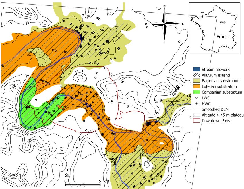
Schirmer et al., 2013). Moreover, the development of levees along the river and riverbed dredging generate major modifications
     of the stream-aquifer status. So far, all those aspects have not been taken into account in water table mapping methodologies.
       The most commonly used methods for the estimation of a continuous variable are linear estimators, neural network and
     kriging (Varouchakis and Hristopulos, 2013). The main linear estimators are inverse distance weighting (Gambolati and Volpi
5    1979, Philip and Watson 1986, Rouhani 1986, Buchanan and Triantafilis 2009, Sun et al. 2009) and influence polygon or
     moving average (Vicente-Serrano et al., 2003). Varouchakis and Hristopulos (2013) compared these different methodologies
     and showed that kriging provides better performance in terms of cross-validation than other linear interpolators. Although the
     linear estimation methods provide unbiased results, they do not account for the spatial heterogeneity of the samples distribution.
     The estimated value depends either on the nearest sampled value (influence polygon), or on every sampled values surrounding
10   the estimation point (moving average) regardless the distance between the estimation point and each individual sampling point.
     Inverse distance weighting involves the arbitrary choice of the distance degree. The distance degree is a conditioning setting
     for the variability of estimated fields whereas kriging involves a weighting of observation that is consistent with the spatial
     distribution of the variable.
       Recently, interpolations based on fuzzy logic or neural network derived methods have been tested (Bresciani et al., 2018;
15   Kurtulus and Flipo, 2012; Sun et al., 2009). These methods are still suffering of a main drawback, that is they produce results
     without coherent spatial error structures (Flipo and Kurtulus, 2011).
       A widely accepted solution that provides information on estimation errors is kriging (Chilès and Delfiner, 1999; Matheron,
     1955). It can be applied on different types of variables (Cressie, 1990) including water table (Hoeksema et al., 1989). Many
     studies produced water table maps resulting from kriging in order to describe water table distributions (Ahmadi and Sedghamiz,
20   2007; Bhat et al., 2014; Buchanan and Triantafilis, 2009; Chung and Rogers, 2012; Hentati et al., 2016; Hoeksema et al.,
     1989; Kurtulus and Flipo, 2012; Mouhri et al., 2013; Zhang et al., 2018). Rouhani and Myers (1990) noticed that water table
     data displays spatial nonstationarities, which are due to the topographic slope. Such nonstationarities cause problems in the
     determination of the experimental variogram and also generate large standard deviations of the estimation errors. A way to
     overcome the issues linked to nonstationarities was proposed by Desbarats et al. (2002). Their methodology also based on
25   kriging was developed for an unconfined aquifer. It relies on the spatial correlation between the water table and the topographic
     surface (King, 1899; Toth, 1962). This assumption was established by Desbarats et al. (2002) at large scales considering several
     watersheds, thereafter, Haitjema and Mitchell-Bruker (2005) proposed that this assumption could be admitted in environments
     with shallow groundwater and smooth topography. This methodology, that targets the unsaturated zone depth (UZD) instead
     of the hydraulic head, leads to lower values of the standard deviation of the estimation error for unconfined aquifer in non-
30   urbanized area (Kurtulus and Flipo, 2012; Mouhri et al., 2013; Rivest et al., 2008; Sağir and Kurtuluş, 2017).
       In urbanized area, the pumping of GW implies the decline of water table, which could lead to the drying out of a few
     piezometers. The knowledge of a dry well can be added to a dataset in the form of an inequality (i.e. UZD larger than the
     well depth) (Michalak, 2008). The counter part of accounting for such information translated into a mathematical inequality
     is that it is incompatible with kriging itself. Therefore another methodology has to be used for water table mapping in such
35   environments.

                                                                     2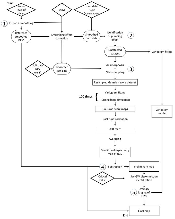
A solution is the usage of multiple conditional simulations that provides a conditional expectancy map of the variable. Its
     application in hydrogeology was demonstrated for hydrofacies determination (Dagan, 1982), converting lithofacies into hydro-
     facies to constrain groundwater flow models. This study proved that the use of conditional probability reduces the variance of
     possible values of the targeted variable, for instance here hydrofacies properties. This methodology was applied in different
5    geological contexts (Tsai and Li, 2007; Dafflon et al., 2008) proving its robustness and has not been applied to the UZD so far.
         The mapping methodology presented in this paper relies on the assumption that the UZD variable is related to the topographic
     elevation and the river water level. The second assumption is that UZD is not related to the stream water level in the case of
     a disconnected hyporheic zone. Therefore, it can be applied to superficial aquifer units submitted to human pressures and
     other locations where the SW-GW connectivity is uncertain. The following questions are addressed: (i) which methodological
10   steps are required for water table mapping in alluvial plains? (ii) how to account for human practices such as pumping in the
     mapping methodology ? (iii) how to determine the SW-GW connection status? (iv) finally, what are the consequences of such
     methodological refinements on produced maps of water table linked to hydrological events?

     2     Mapping Methodology

     Water table mapping was initially developed for the description of regional aquifers into natural or pristine environments.
15   The usual way of mapping a water table is to use synchronous UZD measurements resulting from snapshot campaigns. The
     synchronization of measurements is crucial to avoid experimental bias (Tóth, 2002). This section describes a methodology
     that combines conditional simulations of UZD, with an assessment of SW-GW connectivity and a final ordinary kriging of the
     UZD. Geostatistical processings are performed using the RGeostats R package (Renard et al., 2001 - 2019).
         Fig. 1. describes the methodology. Firstly, the raw dataset is composed of each measured UZD for the corresponding mea-
20   surement campaign. The raw dataset is then transformed into a Gaussian score dataset using an anamorphosis function fitting in
     order to obtain a Gaussian probability density function (Chilès and Delfiner, 1999). Inequality constrained samples (dry wells)
     are estimated using a Gibbs sampling of the Gaussian score subset (Geman and Geman, 1984; Freulon and de Fouquet, 1993).
     Thereafter, one hundred turning band simulations (Matheron, 1973) are performed and averaged before their backtransforma-
     tion into the real data. A first guess map of water table is obtained averaging all back transformed simulations. The SW-GW
25   connectivity status is deduced from the first guess map following a new connectivity criteria that permits to constitute the final
     UZD dataset. The final water table map is finally produced performing an ordinary kriging of the final UZD dataset that is
     removed from a reference Digital Elevation Model (DEM) of the ground.

     2.1    First Guess - Simulations without considering the river water level

     The initial dataset is made of hard data and soft data. The hard data are UZD measured during snapshot campaigns. The soft
30   data are dry well depths. The dataset is characterized in terms of spatial statistics in order to justify the use of an appropriate
     geostatistical tool. UZD is defined in terms of a non-Gaussian probability density function conditioned with non-negativity
     constraint. Unlike water table, UZD can be considered as a continuous stationary variable. The supposed stationarity of a

                                                                     3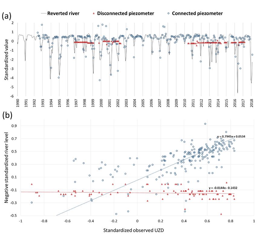
variable makes it usable for ordinary kriging methodologies. In other cases, more complex non-stationary geostatistics should
     be applied, requiring hypothesis about the estimated variable.

     2.1.1   Input data pre-processing & DEM smoothing

     The use of UZD as a variable for mapping the water table requires to refer to the elevation of the ground from which water
5    table can be deduced. In our approach the elevation of the ground is approximated using a smoothed DEM, called reference
     DEM. It is obtained merging a DEM and river water levels. This merged DEM is smoothed (Fig. 1., step 1) using SAGA GIS
     algorithm (Conrad et al., 2015) for moving average filtering. The smoothing of the DEM is required to avoid the occurrence
     of high frequency topography signals that would not be relevant with the water table signal. The search radius is in agreement
     with the average width value of the stream network in order to ensure that the river water level is kept after smoothing. The
10   difference between rough DEM and smoothed DEM may be important in locations where the topographic slope is the most
     important. These locations include crucial areas nearby the riverbanks. Therefore, this difference is calculated at each sampling
     points. Due to the use of UZD, this generates a biased estimation of water table at these locations, given that this difference is
     not yet accounted for into the UZD measured value. The way to tackle the DEM smoothing effect is to constitute a first data
     subset, deducting the difference between DEM data and true wellhead elevation from the raw UZD data before to proceed with
15   the next steps of our procedure (Fig. 1). For the sake of readability, this first data subset will still be called UZD raw dataset in
     the remaining of the paper.

     2.1.2   Hard data selection & variograms

     The variographic analysis of the UZD raw dataset is achieved in order to describe the variability of UZD in a 2D domain. In
     urbanized area, anthropic pressure such as permanent pumping, affects the natural correlation between DEM and UZD with
20   the occurrence of local piezometric depletions. In terms of experimental variogram, the use of samples affected by anthropic
     pressure induces a drastic increase of the semi-variogram value. This cannot be considered as a representative variability of
     the UZD variable. To prevent this effect on the experimental variogram calculation, the original dataset is divided into two
     categories (Fig. 1., step 2). The first category regroups all samples where the UZD value is affected by the pumping wells. The
     second category is composed by the other samples. Information about the locations of pumping wells is required to identify
25   these samples. The observed minimal UZD of depreciated areas can be use as a threshold value to differentiate affected points
     from non-affected points. In this study, the samples with UZD value greater than 10 m are grouped in this category. Note that
     this value may vary according to the case study. This differentiation is required to elaborate a geostatistical tool (i.e. variogram
     model) that only depends of natural variability. Therefore, all the variographic studies are performed on this second category
     called unaffected UZD dataset.
30     The experimental variograms are calculated on two types of variables: the Gaussian score used in the Gibbs sampling and
     conditional simulations, and the unaffected UZD dataset for the final ordinary kriging procedure. The Gaussian score variable
     used for Gibbs sampling-conditionnal simulation steps is described in the next subsections. UZD is the variable ultimately
     used for ordinary kriging. Each calculated experimental variogram is a representation of the spatial variability of the dataset.

                                                                      4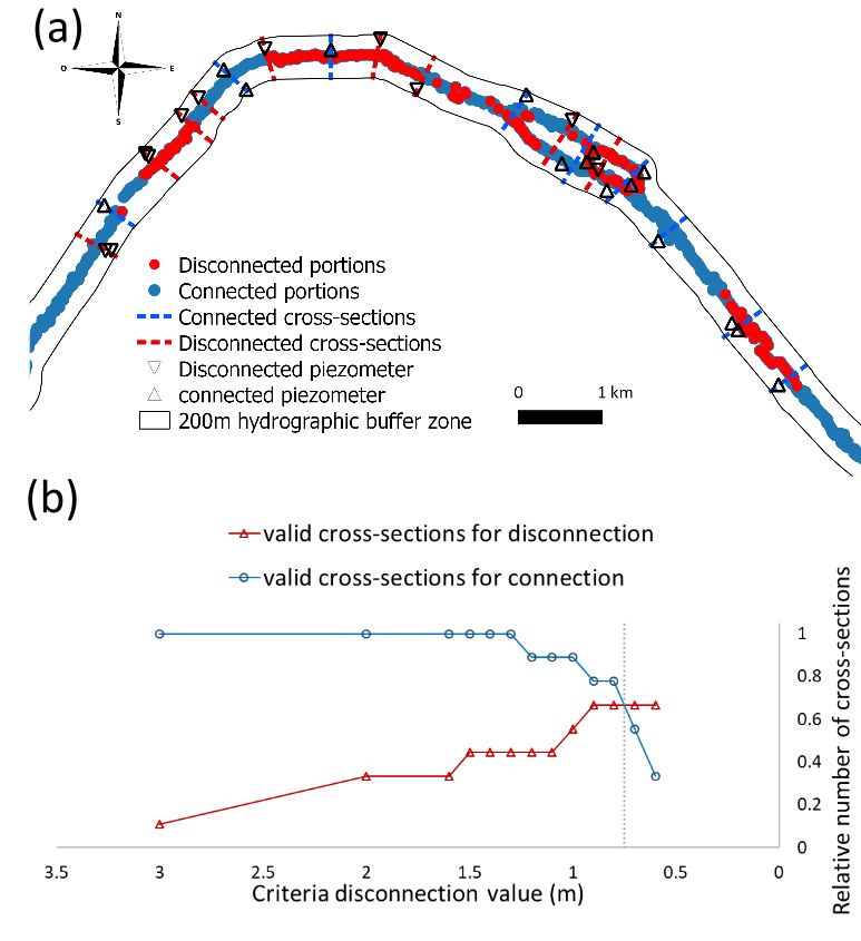
A variogram model is fitted to each experimental variogram with a composition of spherical, exponential and cubic functions.
     The variogram fitting is achieved using an automated procedure (Desassis and Renard, 2013).

     2.1.3   Anamorphosis function fitting

     In order to handle the non-Gaussian behavior of the UZD, one possibility is to transform a random function into a Gaussian
5    function using an anamorphosis function fitting such that ϕ = F −1 ◦G, where ϕ is the anamorphosis function, F the continuous
     marginal distribution function of unaffected UZD, and G the cumulative density function of the Gaussian score (Chilès and
     Delfiner 1999). First, the cumulative histogram of the unaffected UZD dataset is established. Therefore, the corresponding
     Gaussian score is empirically obtained using the frequency inversion of unaffected UZD. The unaffected UZD dataset is
     transformed into a Gaussian score dataset using an anamorphosis function (Fig1. step 3). This transformation was already used
10   by Flipo et al. (2007) to study aquifer contamination by nitrates.

     2.1.4   Gibbs sampling - Including soft data

     A dry well corresponds to soft data that can be formulated as constrained by an inequality. One way to deal with these data
     is to use Gibbs sampling in order to propose a realistic UZD value in accordance with the inequality. The Gibbs sampling
     method is a way to produce a realization of a Markov random field at a given location (Geman and Geman 1984, Freulon and
15   de Fouquet 1993). This methodology can be directly applied to UZD data (Michalak, 2008) in order to provide a value at each
     dry well. In this study, Gibbs sampling is applied to the Gaussian score dataset in order to obtain a re-sampled Gaussian score
     value at each dry well (Fig. 1., step 3). This is made through the distinction between dry well bottom levels (soft data) and
     UZD measurements (hard data). The UZD measurements are accounted as equality constrained samples and dry well bottom
     levels are accounted as inequality constrained samples, constituting a lower limit for UZD value, or in other words a minimum
20   value of UZD at the well location. For each dry well a potential value is calculated from successive simulations that reproduce
     a conditioned value of UZD matching the data distribution and the inequality constraint.
       At the end of the Gibbs sampling, the dry well bottom levels are replaced by a probable UZD value at dry well location. This
     procedure leads to the constitution of a re-sampled Gaussian score dataset.

     2.1.5   Conditional simulations

25   The next step is the spatialization of the Gaussian score dataset using geostatistical simulations. The simulation of a random
     function is the calculation of a possible distribution that matches the variogram and the histogram and that honors the data
     (Journel, 1986). In this study, the simulation is conditioned by the Gaussian score dataset and is performed on a grid covering
     the study area using the Turning Bands method (Matheron, 1973). The used variogram model is the same than the one used for
     Gibbs sampling. Once the simulation is calculated, the resulting Gaussian score map is backtransformed into a UZD map.
30     One hundred conditional simulations are performed for the calculation of the first guess of the water table map.

                                                                     5
2.1.6 First guess of the water table distribution
Each Gaussian spatial distribution is backtransformed into a UZD spatial distribution. A preliminary map is obtained averaging
the 100 conditional UZD distributions. The first guess map of the water table is obtained deducing this preliminary UZD map
from the reference DEM (Fig. 1, step 4).
5 2.2 Water table mapping accounting for uncertain SW-GW connectivity
The second part of the mapping methodology is the final mapping of water table, with the consideration of the SW-GW
connection status: the connection status is evaluated for each cell located below the river network using a new disconnection
criteria.
2.2.1 Defining a disconnection criteria at the reach scale
10 Stream-aquifer systems fluctuate from a hydraulically connected to a disconnected state due to the development of an unsatu-
rated zone below the stream bed. During the switching between connection status, the SW-GW connection status is considered
as a transitional state, this condition can occur when the capillary zone intersects the riverbed (Brunner et al., 2009). The dis-
connected SW-GW condition can occur under different settings such as in case of high hydraulic conductivity contrast between
the clogging layer and the aquifer (Brunner et al., 2009; Peterson and Wilson, 1988), the lowering of the water table (Dillon
15 and Liggett, 1983; Fox and Durnford, 2003; Osman and Bruen, 2002; Rivière et al., 2014; Wang et al., 2011)) or the biological
clogging of the riverbed (Newcomer et al., 2016, 2018; Xian et al., 2019). Considering a constant river water level and river
width, the disconnection occurs when any further increase of the hydraulic head difference between the water table and the
river water level does not affect the infiltration rate from the stream to the underlying aquifer, which remains constant. Wang
et al. (2011) and Rivière et al. (2014) proved that the disconnected state is reached when the saturation profile between the
20 riverbed and the water table is stabilized. The saturation profile fills the space between an inverted area below the riverbed
and a capillary fringe above the water table (Rivière et al., 2014; Wang et al., 2011). In the methodology, we assume that the
disconnection state is reached when these two capillary fringes are separated. The thickness of these two areas is controlled
by the capillary effect which mainly depends on the lithology of both the riverbed and the aquifer. Gillham (1984) proposed
values for capillary fringe heights for several lithologies resulting from experimental measurements (Tab. 1). The disconnection
25 criteria is defined as the distance between the riverbed and water table above which the river water and the groundwater are
disconnected. It means that for higher distances, a saturation profile develops between the inverted area below the riverbed and
the capillary fringe overlying the water table. Accordingly, the disconnection state is identified for a given lithology at each
river cell of the estimation grid, when the difference between the first guess water table and the riverbed elevation equals or
exceeds an empirical disconnection criteria. The methodology therefore requires either an explicit bathymetric description of
30 the river or an estimation of the riverbed elevation.
Starting from the knowledge the riverbed lithology, the disconnection criteria can be estimated from Gillham (1984), this first
guess is uncertain given that the distribution of sedimentary heterogeneities into the alluvial plain induces important lithological
6Table 1. Values for the capillary fringe height, regarding the lithology, after Gillham (1984)
Sand Silt Clay
Height of capillary fringe (m) 0.1 - 1 1 - 10 >10
contrasts (Jordan and Pryor 1992; Flipo et al. 2014) and characterizing such heterogeneities requires important geophysical
surveys that are out of reach for the development of our methodology. At a station, lithology is hence uncertain and a fortiori
even more uncertain along a river reach. However, the disconnection criteria is defined as a threshold difference value between
measured UZD and river water level from which the SW-GW connection status switches. In the absence of such criteria in
5 the literature, an optimisation procedure is proposed along the Seine river network given that piezometers are available in
the vicinity of the river and that both in-river water level and water table in the piezometers are recorded synchronously. The
optimization procedure is described into the application section since it is based on the use of temporal data that is not directly
required for the mapping methodology.
If the two signals are correlated it indicates that the river and the aquifer are connected. Contrarily, a very low correlation
10 indicates a disconnection. At the reach scale, many piezometers are available. The standardized and normalized hydraulic head
and river water level are compared to assess the local connection status of SW-GW. On a scattered plot, the disconnection
appears below a given slope of the regression line.
At a reach scale it is therefore possible to inform the connection status locally (at few stations). Along the river, the distance
between the riverbed and the water table is evaluated from the first guess map. The disconnection criteria is evaluated within a
15 range defined by Gillham (1984) as the one that reproduces the most of the locally assessed connection status. In the absence
of data, the disconnection criteria defined in our study can be used as a first guess.
2.2.2 Final step of the mapping methodology
Disconnected portions of river are deduced from the preliminary water table map with the application of the disconnection
criteria. A final dataset of UZD is then created from the UZD first guess at each sampling location, to which connected river
20 sections are added with a nil UZD value. An ordinary kriging is performed with this final UZD dataset (Fig. 1, step 5) for
which a variogram model is fitted using the UZD data that is not affected by permanent pumping, as it is described in section
2.1.2 (Fig. 2., b. and d.). The kriging methodology consists into solving the following two equations system :
Z ∗ = P λα Zα + mλm
α
P
V arR = C00 −
α λα Cα0
7Where Z ∗ is the estimation, α is the observation point, λα and λm are the weights for observation point and mean value,
R is the residual value (i.e. absolute error), C00 and C0α are the covariance function values for the origin and the α point.
Therefore, the value of R is not determined solving this system, only the variance of R is calculated.
The final water table map is obtained using the reference DEM, from which the UZD kriged map is deduced.
5 3 Results – Water table mapping of Paris urban area
The methodology is demonstrated on the Paris urban area. This urban area covers 900 km2 and includes Paris city and its
closest peripheral suburbs.
3.1 Paris urban area
The Seine and Marne rivers constitute a meandering fluvial system flowing from the South-East to the North-West (Fig. 3).
10 The confluence between the Marne and the Seine River is located in the South-East of the studied area.
The alluvial plain of the Seine and Marne rivers is overlying incised valleys of Eocene to Oligocene sedimentary series,
exposing late Lutetian limestones in the south of the study area and early Bartonian limestones in the north (Fig. 3). Alluvial
sediments constitute the alluvial aquifer and substratum of the Seine and Marne rivers. Lutetian and Bartonian limestones are
underlying aquifers which are separated by thin heterogeneous and discontinuous formations with low hydraulic conductivity.
15 The high proportion of soil sealed areas and the proliferation of pumping wells due to the urbanization, reduces the infiltration
of rainfall, making the anthropogenic pressure the main controlling factor of water table and SW-GW connection status.
Water table have been monitored by water managers since the 1970’s in central Paris area and since the 2000’s in suburb
areas. Water managers noticed that water table of alluvial aquifer in the central area is usually stable at very low levels such
that drying out of superficial aquifers may occur. The water table of peripheral areas remains unaffected by such water table
20 drawdown.
Regardless of the groundwater context, the Seine river is fully embanked, and the river bottom is periodically dredged for
navigation purposes along the Paris city crossing. Given those anthropogenic forcings, water managers suspect that the Seine
river may be disconnected from its underlying alluvial aquifer in some parts of Paris central area. The interpretations of the join
response of alluvial aquifer to hydrological events during the 1990-2018 period described further are supported by monthly
25 records for UZD at monitored piezometers located nearby the Seine river. Seine river water levels vary under two different
hydrological regimes (Fig. 4.a.): one nominal hydrological regime, corresponding to the low flow periods during which the
river flow and water level are artificially regulated for navigation and water management purposes, and one flood regime
during which the river water level reaches the flood peak (eventually causing flood damages). The UZD can vary in relation
with the Seine river water level or not. In the case of no variation of UZD, it is assumed that UZD is regulated by the GW
30 pumpings, inducing a disconnection between water table and river water level.
8Table 2. Overview of the used samples for the application of water table mapping
Total number Number of wells number
of wells affected by pumping wells of dry wells
LWC 314 25 47
HWC 202 33 11
3.2 UZD datasets: Low and High flow campaigns
This study is based on two UZD snapshot campaigns (Tab. 2) involving measurements in piezometers that are not periodically
monitored (Fig. 3): the low water campaign (LWC), that gathered 314 measurements during the low flow period of October
2015, and the high water campaign (HWC), gathering 202 measurements during the June 2016 flood event. Both campaigns last
5 about a week. HWC took place a few days after the flood peak (1750 m3 .s−1 ) was reached at the Parisian Austerlitz gauging
station. The two datasets include around 22 % of samples affected by anthropic pressure (pumping wells and underground
structure) (Tab. 2). Most of these samples are located in the Paris central area where the water table is affected by permanent
pumping.
3.3 Reference DEM for each campaign
10 The used DEM is the IGN scan 25 (IGN, 2015). As previously mentioned, the DEM is first merged with hydrological data
specific for each campaign. Then it is smoothed using a 325 m research radius for moving average filtering.
River water levels are deduced from the recorded data of six discharge gauging stations. The distribution of river water
levels is interpolated using a constant gradient between each gauging station. During low flow period, the average gradient
value is 0.01‰. The Seine River discharge is regulated through a series of locks and dams for navigation purposes. At each
15 lock station, water levels are maintained at a given elevation below a threshold water flow of 600 m3 .s−1 at the Paris Austerlitz
station. When a flood occurs as in June 2016, the lock stations are opened, and the water surface returns to its natural 0.2 ‰
gradient. During the LWC, the Seine river discharge was 160 m3 .s−1 , so that all locks were up, while they were open during
the HWC, when the average discharge still reached 1000 m3 .s−1 a week after the flood peak.
3.4 Variograms
20 The experimental variograms, and the associated fitted variogram models are depicted (Fig. 2). For both datasets, the shape of
the variograms is similar with a sharp increase of the semi-variance nearby the origin, followed by a smooth evolution until it
reaches the sill value. The range is higher for the LWC than for the HWC. The range of the Gaussian score is 12 km for LWC
and 5 km for HWC (Fig. 2.a. & b.). The range of the raw data is 2 km for HWC while it is 6 km for the LWC. It can be noted
that the variographic models for unaffected UZD data differ between LWC and HWC datasets in terms of sill value (Fig. 2.a.
9& b.). The sill value for the variogram model of the unaffected UZD HWC dataset is 8 m2 while it is 5 m2 for the unaffected
UZD LWC dataset. This can be due to either the lower number of samples collected during the HWC, or to variations in the
inner structure of the flow propagation process (Chen et al., 2018; Samine Montazem et al., 2019). For both campaigns (LWC
and HWC), the variogram models of Gaussian scores have a range larger than the one of unaffected UZD datasets. This is due
5 to the increase of the spatial correlation of the variable once the unaffected UZD data is transformed into Gaussian data.
3.5 Assessing the disconnection criteria
The Gaussian simulations are run on a 25 m x 25 m grid that matches the DEM resolution. The average of the hundred UZD
values is subtracted to the smoothed DEM that includes river water levels evaluated for each hydrological context (LWC and
HWC). The streambed of the Seine river consists of mixed fine sand, and silt. The a priory capillary fringe height is comprised
10 within 0.1 m and 1.0 m (Tab. 1). Therefore, the a priory value for the disconnection criteria is comprised between 0.2 m and 2
m. The available observed data is composed of monthly measurements of UZD among 26 piezometers during the 1990-2018
period. These piezometers are distributed along 18 cross-sections of the Seine river. For each piezometer, standardized UZD
and river water level values are calculated. As described in section 2.2.1, the SW-GW connection status can be deduced from
the relation between UZD and river water level. Two classes of piezometers are identified given the linear regression between
15 standardized UZD and standardized river water level: disconnected piezometers and connected piezometers. Please note that
during disconnection, the flow rate is still related to the hydraulic head difference. The disconnection cases are therefore
included in the connected piezometer group. In case of a significant slope of the regression line (>0.57), the piezometer
is considered connected. It is disconnected otherwise. 15 piezometers are considered as connected and 11 piezometers are
considered as disconnected. Therefore, 9 cross-sections along the Seine river are connected and 9 sections are disconnected
20 (Fig. 5.a.).
As an example, two contrasted situations among the 26 piezometers are displayed (Fig. 4.a.). The UZD measured in the blue
piezometer is linearly related to the river water level, while the UZD measured in the red piezometer remains roughly constant.
There is a linear regression between UZD measured in the blue piezometer (Fig. 4.b.) which confirms that the blue piezometer
is connected. In the case of disconnected piezometers, a constant UZD value is measured for most samples. It indicates that
25 UZD is regulated artificially (Fig. 4.a.).
3.6 Sensitivity analysis of the disconnection criteria
The distribution of SW-GW connection status is constrained by the disconnection criteria. To estimate this criteria, a sensitivity
analysis is achieved. The tested values range from 3 m to 0.5 m with a 0.1 m step. This analysis shows that it is not possible to
validate the connection status for all cross-sections. Therefore, we compare the relative numbers of matched connected cross-
30 sections and disconnected cross-sections. When the relative numbers are equal, the optimal value is reached, maximizing the
total number of sections for which the connectivity status is correctly predicted. This optimal value is 0.75 m (Fig. 5.b.). This
value is used to obtain the final water table maps. The value of the disconnection criteria impacts the length of disconnected
reaches. When the value for disconnection criteria is overestimated, the length of disconnected reach is underestimated. Con-
10trarily, when the value is underestimated, the length of disconnected reaches is overestimated. In the application presented here
for LWC, the length of disconnected reach for a 3m disconnection criteria value is 150 m in the central area, while it reaches
a 6 km length when the disconnection occurs for a 0.25m disconnection criteria. When the optimal value of 0.75 m is applied
for disconnection criteria, the length of disconnect reach is 5 km.
5 Further investigation could be carried out to evaluate the reliability of the estimated disconnection criteria, comparing it with
the application of other methodologies such as it is described in Lamontagne et al. (2014). Thought this would allow for the
determination of SW-GW flowrate and hydrogeological dynamics, it cannot be applied into our case study context given that
there is no data about the riverbed hydraulic conductivity. Such development would constitute a supplementary step after the
water table mapping toward the description of the hydrological functioning of the study area.
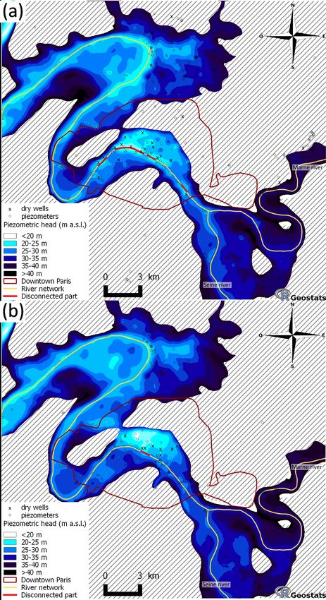
10 3.7 Final mapping integrating SW-GW connectivity
The most important GW hydraulic gradient (1 %) are located close to the Seine and Marne rivers and the areas with an important
topographic gradient (Fig. 6). The lowest values of hydraulic gradient are comprised between 0.1 ‰ and 1 ‰ with an average
0.6 ‰ value in rather flat alluvial plains in the north area and the south-east area. The global flow pattern is therefore driven by
SW-GW connection status and topography, at the exception of the central area where permanent pumping generates significant
15 water drawdown and a subsequent SW-GW disconnection. In this area, the difference between riverbed elevation and estimated
water table is 4 m. The implementation of disconnected reach during final mapping is a key element to reflect the specificity
of urban groundwater such as water drawdown caused by pumping wells. The mapped water table nearby disconnected reach
is only affected by the observed depletion of water table in wells and dry wells. All disconnected sections are located in the
central area during both campaigns. The rise in river water levels during HWC modifies the water table map significantly,
20 especially in the vicinity of the river. The main effect of such hydrological events though the increase of the hydraulic head
is to favor river infiltration towards the aquifer. As a consequence, almost the whole river network is reconnected to the GW,
leading to a rise of the mapped water table. As pumping is increased during a flood to avoid damages against the buildings and
underground infrastructures, a small portion of the Seine River remains disconnected in central Paris (0.75 km, see Fig. 6.b.)
4 Conclusions
25 This study demonstrates an application for an innovative and generic mapping methodology of the water table in an urbanized
alluvial environment. Besides accounting for information brought by the knowledge of dry well locations and depth, the
methodology introduces a SW-GW disconnection criteria for the first time in water table mapping.
The methodology is demonstrated for the case of the Paris urban area, for which it confirms GW managers suspicion for a
disconnection between SW and GW Downtown Paris. Indeed, the water table appears to be locally depleted causing SW-GW
30 disconnection with the alluvial aquifer. Water table maps lead to the identification of spatialized SW-GW disconnected portions
in the central area of the city. In the case of connected SW-GW, an important hydraulic gradient is observed in the vicinity of
the river. In the case of a disconnected state, the water table remains unaffected by the hydrographic network and follows the
11natural slope of the DEM. Such methodology offers the opportunity of an automated water table mapping connected with GW
monitoring network in urbanized areas exposed to flood risk.
Acknowledgements. This study has been carried with the support of the Programme d’Actions de Prévention des Inondations de la Seine et de
la Marne franciliennes (PAPI SMF) steered by the Etablissement Public Territorial de Bassin Seine Grands Lacs (EPTB SGL, the Seine basin
5 institution for river water flow regulation). The used synchronous datasets were produced and kindly provided by the Inspection Générale
des Carrières (IGC, Mairie de Paris) and the other stakeholders involved in that program (Société du Grand Paris, Conseil départementaux de
Seine Saint-Denis et du Val de Marne, RATP, CEREMA). We want to address special thanks to A.M. Prunier-Leparmentier and S. Ventura-
Mostacchi (IGC, Mairie de Paris) for their constant commitment and advices on water table monitoring in Paris city. This monitoring is a key
point for the analysis of piezometric head time-series. Their technical expertise about Paris city groundwater was also a major contribution
10 to this publication. This work is also a contribution to the PIREN Seine research program on the Seine basin, part of the Long Term Socio
Ecological Research (LTSER), french infrastructure Zone Atelier Seine.
12Figures
13Figure 1. Flow chart for the mapping of water table. Steps 1 to 4 for first guess map. Step 5 for the final map. UZD: unsaturated zone depth.
Diamonds display raw data, ellipses display input data after pre-processing and squares display intermediary products.
14Figure 2. Experimental variogram and fitted variogram model of unaffected UZD data and Gaussian score, for LWC dataset in the left
column (a., b.) and HWC dataset in the right column (c., d.)
15Figure 3. Alluvial plain and regional substratum of the Paris urban area. piezometers location for the two campaigns: low water campaign
(LWC) and high water campaign (HWC).
16Figure 4. Temporal analysis charts for SW-GW connection status determination: (a) recorded time-series for river, disconnected piezometer
and connected piezometer; (b) relationship between standardized river level and UZD for disconnected piezometer and connected piezometer.
17Figure 5. Graphical representation for disconnection criteria adjustment: (a) map of observed SW-GW status related to estimated SW-
GW connection status using the optimal 0.75 m value for disconnection criteria; (b) Number of valid SW-GW connection status out of 9
disconnected cross-sections and 9 connected cross-sections.
18Figure 6. Final water table maps obtained using ordinary kriging of UZD deduced from the reference DEM for a) LWC and b) HWC. The
disconnected reaches of the river network are indicated in red for a disconnection criteria of 0.75 m
19References
Ahmadi, S. H. and Sedghamiz, A.: Geostatistical Analysis of Spatial and Temporal Variations of Groundwater Level, Environmental Moni-
toring and Assessment, 129, 277–294, https://doi.org/10.1007/s10661-006-9361-z, 2007.
Attard, G., Winiarski, T., Rossier, Y., and Eisenlohr, L.: Review: Impact of underground structures on the flow of urban groundwater,
5 Hydrogeology Journal, 24, 5–19, https://doi.org/10.1007/s10040-015-1317-3, 2016.
Bhat, S., Motz, L. H., Pathak, C., and Kuebler, L.: Geostatistics-based groundwater-level monitoring network design and its application to the
Upper Floridan aquifer, USA, Environmental Monitoring and Assessment, 187, 4183, https://doi.org/10.1007/s10661-014-4183-x, 2014.
Bresciani, E., Goderniaux, P., and Batelaan, O.: Hydrogeological controls of water table-land surface interactions, Geophysical Research
Letters, 43, 9653–9661, 2016.
10 Bresciani, E., Cranswick, R. H., Banks, E. W., Batlle-Aguilar, J., Cook, P. G., and Batelaan, O.: Using hydraulic head, chloride and electrical
conductivity data to distinguish between mountain-front and mountain-block recharge to basin aquifers, Hydrology and Earth System
Sciences, 22, 1629–1648, https://doi.org/10.5194/hess-22-1629-2018, https://www.hydrol-earth-syst-sci.net/22/1629/2018/, 2018.
Brunner, P., Cook, P. G., and Simmons, C. T.: Hydrogeologic controls on disconnection between surface water and groundwater, Water
Resources Research, 45, n/a–n/a, https://doi.org/10.1029/2008WR006953, w01422, 2009.
15 Buchanan, S. and Triantafilis, J.: Mapping Water Table Depth Using Geophysical and Environmental Variables, Ground Water, 47, 80–96,
https://doi.org/10.1111/j.1745-6584.2008.00490.x, 2009.
Chen, S., Garambois, P.-A., Finaud-Guyot, P., Dellinger, G., Mosé, R., Terfous, A., and Ghenaim, A.: Variance based sensitivity anal-
ysis of 1D and 2D hydraulic models: An experimental urban flood case, Environmental Modelling & Software, 109, 167 – 181,
https://doi.org/https://doi.org/10.1016/j.envsoft.2018.08.008, 2018.
20 Chilès, J.-P. and Delfiner, P.: GEOSTATISTICS Modeling Spatial Uncertainty, Wiley series in probability and statistics, John Wiley & Sons,
Inc., 1999.
Chung, J.-w. and Rogers, J. D.: Interpolations of Groundwater Table Elevation in Dissected Uplands, Groundwater, 50, 598–607,
https://doi.org/10.1111/j.1745-6584.2011.00889.x, 2012.
Conrad, O., Bechtel, B., Bock, M., Dietrich, H., Fischer, E., Gerlitz, L., Wehberg, J., Wichmann, V., and Böhner, J.: System for Automated
25 Geoscientific Analyses (SAGA) v. 2.1.4, Geoscientific Model Development, 8, 1991–2007, https://doi.org/10.5194/gmd-8-1991-2015,
2015.
Cressie, N.: The origins of kriging, Mathematical Geology, 22, 239–252, https://doi.org/10.1007/BF00889887, 1990.
Dafflon, B., Irving, J., and Holliger, K.: Use of high-resolution geophysical data to characterize heterogeneous aquifers: Influence of data
integration method on hydrological predictions, Water Resources Research, 45, https://doi.org/10.1029/2008WR007646, https://agupubs.
30 onlinelibrary.wiley.com/doi/abs/10.1029/2008WR007646, 2008.
Dagan, G.: Stochastic modeling of groundwater flow by unconditional and conditional probabilities: 1. Conditional simulation and the direct
problem, Water Resources Research, 18, 813–833, https://doi.org/10.1029/WR018i004p00813, 1982.
Desassis, N. and Renard, D.: Automatic Variogram Modeling by Iterative Least Squares: Univariate and Multivariate Cases, Mathematical
Geosciences, 45, 453–470, https://doi.org/10.1007/s11004-012-9434-1, 2013.
35 Desbarats, A., Logan, C., Hinton, M., and Sharpe, D.: On the kriging of water table elevations using collateral information from a digital
elevation model, Journal of Hydrology, 255, 25 – 38, https://doi.org/https://doi.org/10.1016/S0022-1694(01)00504-2, 2002.
20Dillon, P. J. and Liggett, J. A.: An ephemeral stream-aquifer interaction model, Water Resources Research, 19, 621–626,
https://doi.org/10.1029/WR019i003p00621, https://agupubs.onlinelibrary.wiley.com/doi/abs/10.1029/WR019i003p00621, 1983.
Flipo, N. and Kurtulus, B.: GEO - ANFIS : Application to piezometric head interpolation in unconfined aquifer unit, in: Proceedings of
FUZZYSS’11, p. 6p., 2011.
5 Flipo, N., Jeannée, N., Poulin, M., Even, S., and Ledoux, E.: Assessment of nitrate pollution in the Grand Morin aquifers (France): combined
use of geostatistics and physically-based modeling, 146, 241–256, https://doi.org/10.1016/j.envpol.2006.03.056, 2007.
Flipo, N., Mouhri, A., Labarthe, B., Biancamaria, S., Rivière, A., and Weill, P.: Continental hydrosystem modelling : the concept of nested
stream-aquifer interfaces, Hydrology and Earth System Sciences, 18, 3121–3149, https://doi.org/10.5194/hess-18-3121-2014, 2014.
Fox, G. A. and Durnford, D. S.: Unsaturated hyporheic zone flow in stream/aquifer conjunctive systems, Advances in Water Re-
10 sources, 26, 989 – 1000, https://doi.org/https://doi.org/10.1016/S0309-1708(03)00087-3, http://www.sciencedirect.com/science/article/
pii/S0309170803000873, modeling Hyporheic Zone Processes, 2003.
Freulon, X. and de Fouquet, C.: Conditioning a Gaussian model with inequalities, pp. 201–212, Springer Netherlands, Dordrecht,
https://doi.org/10.1007/978-94-011-1739-5_17, https://doi.org/10.1007/978-94-011-1739-5_17, 1993.
Gambolati, G. and Volpi, G.: A conceptual deterministic analysis of the kriging technique in hydrology, Water Resources Research, 15, 625–
15 629, https://doi.org/10.1029/WR015i003p00625, https://agupubs.onlinelibrary.wiley.com/doi/abs/10.1029/WR015i003p00625, 1979.
Geman, S. and Geman, D.: Stochastic Relaxation, Gibbs Distributions, and the Bayesian Restoration of Images., IEEE Transactions on
Pattern Analysis and Machine Intelligence, 6, 721–741, 1984.
Gillham, R.: The capillary fringe and its effect on water-table response, Journal of Hydrology, 67, 307 – 324,
https://doi.org/https://doi.org/10.1016/0022-1694(84)90248-8, 1984.
20 Haitjema, H. M. and Mitchell-Bruker, S.: Are Water Tables a Subdued Replica of the Topography?, Ground Water, 43, 781–786,
https://doi.org/10.1111/j.1745-6584.2005.00090.x, 2005.
Hentati, I., Triki, I., Trablesi, N., and Zairi, M.: Piezometry mapping accuracy based on elevation extracted from various spatial data sources,
Environmental Earth Sciences, 75, 802, https://doi.org/10.1007/s12665-016-5589-2, 2016.
Hoeksema, R. J., Clapp, R. B., Thomas, A. L., Hunley, A. E., Farrow, N. D., and Dearstone, K. C.: Cokriging model for estimation of water
25 table elevation, Water Resources Research, 25, 429–438, https://doi.org/10.1029/WR025i003p00429, 1989.
IGN: BD ALTI Version 2.0. Tech. Rep. Institut Géographique National., 2015.
Jordan, D. W. and Pryor, W. A.: Hierarchical levels of heterogeneity in a Mississippi River meander belt and application to reservoir systems:
geologic Note (1), AAPG Bulletin, 76, 1601–1624, 1992.
Journel, A. G.: Constrained interpolation and qualitative information—The soft kriging approach, Mathematical Geology, 18, 269–286,
30 https://doi.org/10.1007/BF00898032, 1986.
King, F. H.: Principles and conditions of the movements of ground water, US Geological Survey 19th Annual Report, Part 2, 59–294, 1899.
Kurtulus, B. and Flipo, N.: Hydraulic head interpolation using anfis - model selection and sensitivity analysis, Computers & Geosciences,
38, 43 – 51, https://doi.org/https://doi.org/10.1016/j.cageo.2011.04.019, 2012.
Lamontagne, S., Taylor, A., Cook, P., Crosbie, R., Brownbill, R., Williams, R., and Brunner, P.: Field assessment of surface
35 water–groundwater connectivity in a semi-arid river basin (Murray–Darling, Australia), Hydrological Processes, 28, 1561–1572,
https://doi.org/10.1002/hyp.9691, https://onlinelibrary.wiley.com/doi/abs/10.1002/hyp.9691, 2014.
21Machiwal, D., Jha, M. K., Singh, V. P., and Mohan, C.: Assessment and mapping of groundwater vulnerability to pollution: Cur-
rent status and challenges, Earth-Science Reviews, 185, 901 – 927, https://doi.org/https://doi.org/10.1016/j.earscirev.2018.08.009, http:
//www.sciencedirect.com/science/article/pii/S0012825217304713, 2018.
Matheron, G.: Application des méthodes statistiques à l’évaluation des gisements, in: Annales des mines, vol. 144, pp. 50–75, 1955.
5 Matheron, G.: The intrinsic random functions and their applications., Advances in Applied Probability, 5, 439–468,
https://doi.org/10.2307/1425829, 1973.
Michalak, A. M.: A Gibbs sampler for inequality-constrained geostatistical interpolation and inverse modeling, Water Resources Research,
44, https://doi.org/10.1029/2007WR006645, 2008.
Morris, B., Lawrence, A., Chilton, P., Adams, B., Calow, R., and Klinck, B.: Groundwater and its susceptibility to degradation : a global
10 assessment of the problem and options for management, vol. 03-3 of Eary warning and assessment report series, United Nations Envi-
ronment Programme, 2003.
Mouhri, A., Flipo, N., Rejiba, F., de Fouquet, C., Bodet, L., Kurtulus, B., Tallec, G., Durand, V., Jost, A., Ansart, P., and Goblet, P.:
Designing a multi-scale sampling system of stream-aquifer interfaces in a sedimentary basin, Journal of Hydrology, 504, 194–206,
https://doi.org/https://doi.org/10.1016/j.jhydrol.2013.09.036, 2013.
15 Newcomer, M. E., Hubbard, S. S., Fleckenstein, J. H., Maier, U., Schmidt, C., Thullner, M., Ulrich, C., Flipo, N., and Rubin,
Y.: Simulating bioclogging effects on dynamic riverbed permeability and infiltration, Water Resources Research, 52, 2883–2900,
https://doi.org/10.1002/2015WR018351, https://agupubs.onlinelibrary.wiley.com/doi/abs/10.1002/2015WR018351, 2016.
Newcomer, M. E., Hubbard, S. S., Fleckenstein, J. H., Maier, U., Schmidt, C., Thullner, M., Ulrich, C., Flipo, N., and Rubin, Y.: Influence of
Hydrological Perturbations and Riverbed Sediment Characteristics on Hyporheic Zone Respiration of CO2 and N2, Journal of Geophysical
20 Research: Biogeosciences, 123, 902–922, https://doi.org/10.1002/2017JG004090, 2018.
Osman, Y. Z. and Bruen, M. P.: Modelling stream–aquifer seepage in an alluvial aquifer: an improved loosing-stream package for MOD-
FLOW, Journal of Hydrology, 264, 69 – 86, https://doi.org/https://doi.org/10.1016/S0022-1694(02)00067-7, http://www.sciencedirect.
com/science/article/pii/S0022169402000677, 2002.
Peterson, D. M. and Wilson, J. L.: Variably saturated flow between streams and aquifers, 1988.
25 Philip, G. and Watson, D.: Automatic interpolation methods for mapping piezometric surfaces, Automatica, 22, 753 –
756, https://doi.org/https://doi.org/10.1016/0005-1098(86)90016-6, http://www.sciencedirect.com/science/article/pii/0005109886900166,
1986.
Renard, D., Bez, N., Desassis, N., Beucher, H., Ors, F., and Freulon, X.: RGeostats: The Geostatistical R package [11.0.5]., free download
from: http://cg.ensmp.fr/rgeostats, 2001 - 2019.
30 Rivest, M., Marcotte, D., and Pasquier, P.: Hydraulic head field estimation using kriging with an external drift: A way to consider conceptual
model information, Journal of Hydrology, 361, 349 – 361, https://doi.org/https://doi.org/10.1016/j.jhydrol.2008.08.006, 2008.
Rivière, A., Gonçalvès, J., Jost, A., and Font, M.: Experimental and numerical assessment of transient stream-aquifer exchange during
disconnection, Journal of Hydrology, 517, 574 – 583, https://doi.org/https://doi.org/10.1016/j.jhydrol.2014.05.040, 2014.
Rouhani, S.: Comparative Study of Ground-Water Mapping Techniques, Groundwater, 24, 207–216, https://doi.org/10.1111/j.1745-
35 6584.1986.tb00996.x, https://onlinelibrary.wiley.com/doi/abs/10.1111/j.1745-6584.1986.tb00996.x, 1986.
Rouhani, S. and Myers, D. E.: Problems in space-time kriging of geohydrological data, Mathematical Geology, 22, 611–623,
https://doi.org/10.1007/BF00890508, 1990.
22Sağir, Ç. and Kurtuluş, B.: Hydraulic head and groundwater 111Cd content interpolations using empirical Bayesian kriging (EBK) and
geo-adaptive neuro-fuzzy inference system (geo-ANFIS), Water SA, 43, 509–519, https://doi.org/http://dx.doi.org/10.4314/wsa.v43i3.16,
2017.
Samine Montazem, A., Garambois, P.-A., Calmant, S., Finaud-Guyot, P., Monnier, J., Medeiros Moreira, D., Minear, J. T., and Biancamaria,
5 S.: Wavelet-Based River Segmentation Using Hydraulic Control-Preserving Water Surface Elevation Profile Properties, Geophysical Re-
search Letters, 46, 6534–6543, https://doi.org/10.1029/2019GL082986, 2019.
Schirmer, M., Leschik, S., and Musolff, A.: Current research in urban hydrogeology – A review, Advances in Water Re-
sources, 51, 280 – 291, https://doi.org/https://doi.org/10.1016/j.advwatres.2012.06.015, http://www.sciencedirect.com/science/article/pii/
S0309170812001790, 35th Year Anniversary Issue, 2013.
10 Sun, Y., Kang, S., Li, F., and Zhang, L.: Comparison of interpolation methods for depth to groundwater and its tempo-
ral and spatial variations in the Minqin oasis of northwest China, Environmental Modelling & Software, 24, 1163 – 1170,
https://doi.org/https://doi.org/10.1016/j.envsoft.2009.03.009, 2009.
Toth, J.: A theory of groundwater motion in small drainage basins in central Alberta, Canada, Journal of Geophysical Research, 67, 4375–
4388, https://doi.org/10.1029/JZ067i011p04375, 1962.
15 Tóth, J.: József Tóth: An Autobiographical Sketch, Groundwater, 40, 320–324, https://doi.org/10.1111/j.1745-6584.2002.tb02661.x, 2002.
Tsai, F. T.-C. and Li, X.: Inverse groundwater modeling for hydraulic conductivity estimation using Bayesian model averaging and vari-
ance window, Water Resources Research, 44, https://doi.org/10.1029/2007WR006576, https://agupubs.onlinelibrary.wiley.com/doi/abs/
10.1029/2007WR006576, 2007.
Varouchakis, E. A. and Hristopulos, D. T.: Comparison of stochastic and deterministic methods for mapping groundwater level spatial
20 variability in sparsely monitored basins, Environmental Monitoring and Assessment, 185, 1–19, https://doi.org/10.1007/s10661-012-2527-
y, https://doi.org/10.1007/s10661-012-2527-y, 2013.
Vicente-Serrano, S. M., Saz-Sánchez, M. A., and Cuadrat, J. M.: Comparative analysis of interpolation methods in the middle Ebro Valley
(Spain): application to annual precipitation and temperature, Climate research, 24, 161–180, 2003.
Wang, W., Li, J., Feng, X., Chen, X., and Yao, K.: Evolution of stream-aquifer hydrologic connectedness during pumping - Experiment,
25 Journal of Hydrology, 402, 401 – 414, https://doi.org/https://doi.org/10.1016/j.jhydrol.2011.03.033, 2011.
Winter, T. C., Harvey, J. W., Franke, O. L., and Alley, W. M.: Ground water and surface water; a single resource, Tech. rep., US Geological
Survey„ 1998.
Xian, Y., Jin, M., Zhan, H., and Liu, Y.: Reactive Transport of Nutrients and Bioclogging During Dynamic Disconnection Process of Stream
and Groundwater, Water Resources Research, 55, 3882–3903, https://doi.org/10.1029/2019WR024826, https://agupubs.onlinelibrary.
30 wiley.com/doi/abs/10.1029/2019WR024826, 2019.
Zhang, X., Guan, T., Zhou, J., Cai, W., Gao, N., Du, H., Jiang, L., Lai, L., and Zheng, Y.: Groundwater Depth and Soil Properties Are Asso-
ciated with Variation in Vegetation of a Desert Riparian Ecosystem in an Arid Area of China, Forests, 9, https://doi.org/10.3390/f9010034,
2018.
23You can also read