Predicting citywide distribution of air pollution using mobile monitoring and three-dimensional urban structure
←
→
Page content transcription
If your browser does not render page correctly, please read the page content below
Preprints (www.preprints.org) | NOT PEER-REVIEWED | Posted: 5 May 2021                    doi:10.20944/preprints202104.0588.v2

                 Predicting citywide distribution of air pollution using mobile monitoring and
                 three-dimensional urban structure

                 Lucas E. Cummings*1, Justin D. Stewart*1,2, Peleg Kremer1, Kabindra.M. Shakya1

                 *These authors contributed to this work equally
                 1
                   Department of Geography and the Environment, Villanova University, Pennsylvania,
                 USA
                 2
                   Department of Ecological Science, Vrije Universiteit Amsterdam, 1081 HV Amsterdam,
                 The Netherlands

                 Abstract

                 Understanding relationships between urban structure patterns and air pollutants is key to
                 sustainable urban planning and development. This study employed mobile monitoring of
                 PM2.5 and BC across ~480 Kilometers in Philadelphia, USA during summer 2019. We
                 apply the 3D Structure of Urban Landscapes (STURLA) classification to examine
                 relationships between urban structure and atmospheric pollution. We find that, while
                 PM2.5 and BC vary by STURLA class, many of the differences in pollutant
                 concentrations between classes are not significant. However, we also find that the
                 proportions in which STURLA components are present throughout the urban landscape
                 can be used to predict urban air pollution. Among frequently sampled STURLA classes,
                 gpl hosted the highest PM2.5 concentrations on average (16.60 ± 4.29 µg/m3), while
                 tgbwp hosted the highest BC concentrations (2.31 ± 1.94 µg/m3). Furthermore, STURLA
                 combined with machine learning modeling was able to correlate PM2.5 (R2= 0.68,
                 RMSE 2.82 µg/m3) and BC (R2 = 0.64, RMSE 0.75 µg/m3) concentrations with the
                 composition of the urban landscape and predict concentrations where sampling did not
                 take place. These results demonstrate the efficacy of the STURLA methodology in
                 modeling relationships between air pollution and urban structure patterns.

                 Significance Statement

                 This study is the first to use the Structure of Urban Landscapes (STURLA) methodology
                 in the context of air pollution modeling to examine relationships between air pollution and
                 urban structure. The study also utilizes big data collected on a large spatial scale (483
                 km throughout Philadelphia) through a mobile monitoring method, which is a relatively

                                                                                                                      1

           © 2021 by the author(s). Distributed under a Creative Commons CC BY license.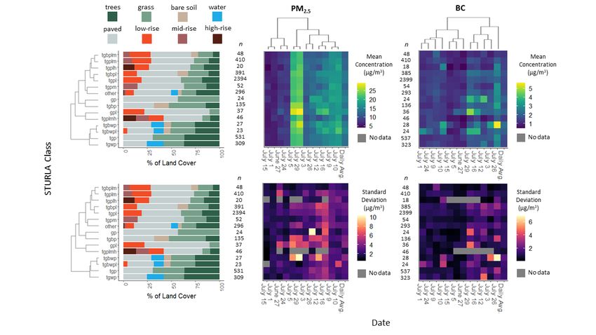
Preprints (www.preprints.org) | NOT PEER-REVIEWED | Posted: 5 May 2021         doi:10.20944/preprints202104.0588.v2

                 new and accessible way to measure pollutant concentrations while providing high levels
                 of spatial and temporal resolution.

                 Main Text

                 Introduction

                          Population growth in urban areas is increasing rapidly; the United Nations
                 projects that 68% of the world’s population will live in urban areas by 2050 (UN DESA,
                 2018). As urban areas expand, a larger proportion of the global population will be
                 exposed to increasingly high and potentially harmful levels of air pollution. At present, 9
                 out of 10 people regularly breathe air containing unsafe level of air pollutants (WHO,
                 2018), and approximately 3.7 million premature deaths worldwide can be attributed to
                 elevated air pollutant concentrations each year (Cohen et al., 2017). Elevated levels of
                 air pollutants disproportionately impact people based on race, (Perlin et al. 1999; Gray et
                 al. 2013), gender and sexual orientation (Collins et al., 2017a; Collins et al., 2017b) and
                 socioeconomic status (Perlin et al. 1999; Zhou et al. 2011; Gray et al. 2013). To ensure
                 that air quality management is equitable and protects the health of urban populations, it
                 is crucial that we understand how air pollutants interact with the urban environment.
                          Particulate matter (PM) has been linked to negative health outcomes, including
                 asthma (Halonen et al., 2008; Anenberg et al. 2018), lung cancer (Hamra et al. 2014;
                 Pope et al. 2002), DNA alteration (Sørensen et al. 2003; Shi et al., 2019; Baccarelli et
                 al., 2009), and disrupted immune function (Zelikoff et al., 2008; Honda et al. 2017).
                 Polluted airs also host potentially pathogenic bacteria (Stewart et al., 2020; Liu et al.,
                 2018) and viruses (Zhu et al., 2020) that may cause disease and aggravate pre-existing
                 conditions. Fine particulate matter (PM2.5) is of significant concern due to its abundance
                 in urban atmospheres, and subsequent potential to cause respiratory and cardiovascular
                 damage (Dockery et al., 1993; Paul et al., 2019; Rabinovitch et al., 2006; Shakya et al.,
                 2016). Black carbon (BC), a subset of PM2.5, is generated through incomplete
                 combustion of fossil fuels and is particularly prevalent in urban areas. Unlike PM2.5,
                 almost all of BC originates from anthropogenic sources, with biomass fires being the
                 only natural source of BC (Hitzenberger & Tohno, 2001); as such, BC is commonly used
                 as an indicator of anthropogenic influence on ambient air pollution (Cyrys et al., 2003;
                 Targino et al., 2016).
                          Studies of urban air pollution have established relationships between landcover,
                 urban structure, and ambient air pollution (Eeftens et al. 2012; Yuan et al. 2019). In
                 urban areas such as Philadelphia, particulate matter concentrations vary across
                 neighborhoods as a result of differences in open space and land structure (Shakya et al.,
                 2019). The organization and height of buildings, barriers and other structures in an urban
                 environment can influence air flow, which in turn impacts local pollutant dispersal
                 (Baldauf et al., 2016; Gallagher et al., 2015; Ng & Chau, 2013). Though many urban
                 areas are characterized by dense built environment, different types of urban green
                 space (e.g. urban forest, parks, gardens, and private yards) are an integral part of the
                 urban landscape. Over the last few decades, cities are increasingly adopting strategies
                 such as urban greening to counteract environmental degradation and enhance human
                 wellbeing. However, these strategies and their efficacy in mitigating urban air pollution
                 are still unclear (Nemitz et al., 2020). While vegetation such as trees and grasses have
                 been shown to reduce air pollution by facilitating pollutant deposition and uptake of
                                                                                                           2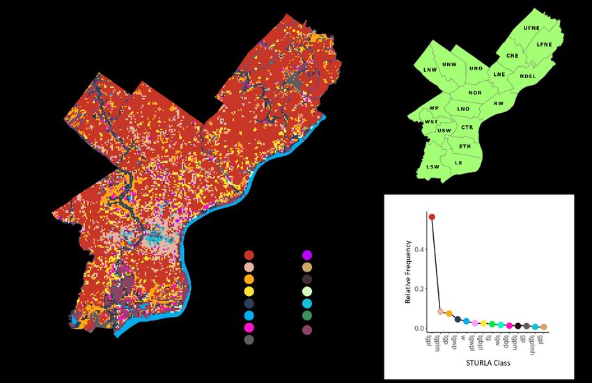
Preprints (www.preprints.org) | NOT PEER-REVIEWED | Posted: 5 May 2021          doi:10.20944/preprints202104.0588.v2

                 particulate matter, they are also capable of causing an increase in local pollutant
                 concentrations through biogenic emissions that serve to facilitate secondary aerosol
                 formation and the inhibition of air flow (Brantley et al. 2014; Chen et al. 2016; Eisenman
                 et al. 2019; Xing & Brimblecombe 2019).
                          Although it is becoming increasingly clear how individual components of urban
                 environments influence air pollution, complex urban topologies make it difficult to
                 understand how these individual components interact to influence air pollution at more
                 localized scales. In urban environments, landcover and urban structure often change
                 drastically over short distances (Cadenasso et al., 2007). While cities may contain
                 common environmental features such as water and greenspace, differences in their
                 organization have varied impacts on air quality. This further complicates efforts to
                 generalize the impact that urban environments have on air pollution. Sustainable
                 development is contingent on reproducible and scalable analyses with geographically
                 meaningful units for urban planning. To this end, there have been efforts to streamline
                 the characterization of cities at smaller scales. The Structure of Urban Landscape
                 (STURLA) composite classification system allows for modeling of three-dimensional
                 urban areas at fine spatial scales. STURLA does so by using fine-scale landcover and
                 building height data to identify common compositions of urban environments (Hamstead
                 et al., 2016). STURLA studies have linked urban landscape structure and land surface
                 temperature (Hamstead et al., 2016; Kremer et al. 2018; Larondelle et al., 2014; Mitz et
                 al., 2021), as well as the phylogenetic diversity of the atmospheric microbiome (Stewart
                 et al. 2021). STURLA allows for meaningful classifications of urban structure and
                 landcover, which have the potential to reshape our understanding of how the
                 composition and spatial organization of urban environments influence environmental
                 parameters. There have also been efforts to improve the accuracy of urban air pollution
                 measurement, as variability in three-dimensional urban landscape composition can
                 influence pollutant dispersal and affect concentrations at small scales (Abhijith &
                 Gokhale, 2015; Gallagher et al. 2015; Hagler et. al, 2012). In recent years, mobile
                 monitoring has been used study the spatiotemporal distribution of air pollutants in cities
                 (Apte et al., 2017; deSouza et al., 2020; Deville Cavellin et al., 2016; Shakya et al.,
                 2019; Sm et al., 2019; Targino et al., 2016; Van Poppel et al., 2013). An advantage of
                 mobile monitoring is that it can collect data at finer spatial scales than is feasible with
                 stationary monitoring (Shakya et al., 2019; Van den Bossche et al., 2015) and
                 subsequent spatial predictions logically should be more accurate and meaningful. In this
                 study, we use data collected through mobile monitoring to measure concentrations of
                 particulate matter smaller than 2.5 µm (PM2.5) and black carbon (BC) throughout the city
                 of Philadelphia over the course of 12 days during the summer of 2019 (Cummings &
                 Stewart et al., 2021). We use STURLA in conjunction with the collected air pollution
                 data to analyze the urban structure-air pollution relationship across the city of
                 Philadelphia.

                 Results

                 Variation in Landscape Structure with PM2.5 and BC Concentrations Among STURLA
                 Classes

                       Differences in both landscape composition and the measured pollutant
                 concentrations they host are evident among the most sampled STURLA classes (Figure

                                                                                                            3
Preprints (www.preprints.org) | NOT PEER-REVIEWED | Posted: 5 May 2021 doi:10.20944/preprints202104.0588.v2
2). Although a slightly different subset of cells was sampled for PM2.5 and BC due to
differences in temporal resolutions of sampling equipment (5 seconds for BC compared
to 6 seconds for PM2.5), differences in average STURLA class composition are minimal
and did not influence clustering between classes. Daily means for PM2.5 among STURLA
classes range from 11.47 ± 1.89 µg/m3 (tgbplm) to 16.60 ± 4.29 µg/m3 µg/m3 (gpl), while
daily means for BC range from 1.25 ± 0.71 µg/m3 (tgbplm) to 2.31 ± 1.94 µg/m3 (tgbwp)
(Figure 2). Permutational t-tests reveal that some of the differences in pollutant
concentrations between STURLA classes are statistically significant (p < 0.05) (Figure
A3). Class gpl demonstrated the most unique PM2.5 signature, with daily mean PM2.5
concentrations differing significantly from six classes: tgp, tgplm, tgwp, tgpm, tgbplm,
and tgplmh. Class tgbplm presented the most distinct BC signature with the daily
average BC concentration being significantly different from four other classes sampled:
tgplmh, gpl, tgbwp, and gp. However, other STURLA classes did not have pollutant
concentrations that were significantly different from other classes. More significant
differences between classes were found with PM2.5 concentrations (17) than with BC
concentrations (9) (Figure A3).
Spatial Modeling of PM2.5 and BC
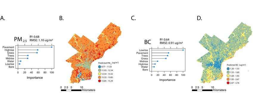
Pavement was the most important variable in modeling PM2.5, followed by high-
rise, grass, trees, mid-rise, water, and low-rise (Figure 3A). In modeling BC, low-rise was
the most important variable, followed by pavement, trees, grass, mid-rise, high-rise, and
water (Figure 3C). In both models, bare soil did not contribute to predictions of pollutant
concentrations (Figures 3A, 3C). Predictions varied by STURLA class. Philadelphia’s
most frequent class, tgpl, has a mean prediction of 13.71 µg/m3; modeling overpredicted
the average measured concentration of the class by 1.64 µg/m3. STURLA classes gbp,
tgp, and gpl are among the classes with the highest predicted concentrations, while pm,
tgwpl, gwp had the lowest (Table A4). Variation in PM2.5 concentrations across the city
were largely explained by differences in sampled STURLA classes (R2 = 0.68, RMSE
1.10 µg/m3). PM2.5 predictions (Figure 3B) ranged from 8.77 – 15.29 µg/m3; actual PM2.5
concentrations by class ranged from 5.40 – 22.21 µg/m3. Differences between STURLA
class composition were slightly less effective in explaining variation in BC concentrations
(R2 = 0.64, RMSE 0.91 µg/m3). BC predictions by class were generally higher than
measured concentrations and ranged from 1.26 µg/m3 to 3.76 µg/m3 (Figure 3D); actual
concentrations by class ranged from 0.85 – 5.45 µg/m3. BC predictions in tgpl hosted
predicted BC values of 1.65 µg/m3 and overpredicted measured BC in tgpl pixels by 0.07
µg/m3. Classes with more internal class elements generally have lower predicted air
pollution concentrations; while tpl, tp, and twpm have the highest BC predictions, tgbph,
tgplmh, and tgbplh have the lowest.
PM2.5 predictions by planning district ranged from 12.62 µg/m3 – 13.74 µg/m3; the
highest predicted PM2.5 concentrations are in the Upper Far Northeast and Lower Far
Northeast planning districts, while the lowest predicted concentrations were found in the
Central planning district (Table A5). 17 of 18 planning districts underpredicted measured
PM2.5 concentrations (Predicted PM2.5 / Measured PM2.5 ratio < 1), which ranged from
12.74 µg/m3 – 14.11 µg/m3 (Table A5). PM2.5 modeling was the most accurate in the
Lower South district (Figure A4B), with a difference of 0.02 µg/m3 between predicted and
measured concentrations, but least accurate in the South district, with a 0.38 µg/m3
difference between predicted and measured concentrations. Overpredictions were less
common than underpredictions by STURLA class PM2.5 with ~44% STURLA classes
4Preprints (www.preprints.org) | NOT PEER-REVIEWED | Posted: 5 May 2021 doi:10.20944/preprints202104.0588.v2
underestimating concentrations (Figure A4A). for Conversely, the model predicted higher
than measured BC concentrations in most STURLA classes (Table A5, Figure A4C)
found in all planning districts (Figure A4D). Predicted BC concentrations ranged from
1.54 µg/m3 – 1.78 µg/m3, while measured BC concentrations ranged from 1.49 µg/m3 –
1.66 µg/m3. BC predictions are highest in the Lower South district and lowest in the
Central district. BC modeling was most effective in the Central, Lower Far Northeast,
North, North Delaware, River Wards, and University Southwest planning districts, all of
which have 0.05 µg/m3 between predicted and measured values; in the Lower South
district, the difference between predicted and measured BC concentrations is at its
highest (0.12 µg/m3).
Discussion
Variation in PM2.5 and BC by STURLA Class
PM2.5 and BC varied by STURLA class (Figure 2); while some classes, such as
gpl and no class had PM2.5 concentrations or BC concentrations that were significantly
different from all commonly sampled classes (Figure A3). Among the 14 most sampled
STURLA classes, we find that the classes containing mid-rise and high-rise buildings
hosted lower concentrations of PM2.5 and BC relative to other commonly sampled
classes; the five classes containing the vertical built environment m or h (tgplm, tgpm,
tgplh, tgplmh, and tgbplm) show the lowest average concentrations of PM2.5 and BC
(Figure 2). Four of these five classes (tgpm, tgplh, tgplmh, and tgbplm) also have the
lowest daily variation in PM2.5 concentrations, while all five have the lowest daily
variation in BC concentrations (Figure 2). While greater proportion of highrise buildings
(Aristodemou et al., 2018) generally host higher air pollution concentrations, the
compositional nature of STURLA may be picking up broader patterns. These classes
also host greenspace, which tend to have lower concentrations of air pollutants (Leung
et al., 2011; Li et al., 2016). A holistic view of greenspace with tall buildings may
represent vegetation mediated pollution removal as well as dispersal limitation. Buildings
restrict air flow and pollutant dispersal, causing an increase in pollutant concentrations
closer to the peak of the building while decreasing concentrations at the ground-level
where sampling occurred (Aristodemou et al., 2018; Zhang et al., 2013). Likewise,
potential sources of PM and BC may simply be less abundant and/or smaller in
magnitude where these classes are found, despite PM concentrations typically being
higher in areas with denser built environment (Zhou & Lin, 2019). It is worth noting that
classes with m and h components were generally sampled less frequently, except for
tgplm, because they are less prevalent in the city’s landscape. Some classes, such as
tgplh and tgplmh, were not sampled enough to be able to quantify variability in pollutant
concentrations on some days (Figure 2). Smaller sample sizes may have been less
effective at capturing the full range of pollutant concentrations for specific classes than
larger sample sizes.
While classes such as tgbplm, tgplm, and tgplh, are compositionally similar and
have similar concentrations of PM2.5 and BC (Figure 2), others display pronounced
differences in pollutant levels despite compositional similarities with other STURLA
classes. Among the most sampled STURLA classes, gpl hosted the highest PM2.5
concentrations and the third-highest BC concentrations. Class gpl is largely dominated
by built environment, with roughly 89.9% of gpl cells characterized by pavement and
low-rise buildings (Figure 2). In class tgplmh, the class most similar to gpl by STURLA
5Preprints (www.preprints.org) | NOT PEER-REVIEWED | Posted: 5 May 2021 doi:10.20944/preprints202104.0588.v2
elements, we observe the second-lowest daily average PM2.5 and BC concentrations
throughout the sampling period. Conversely, class gp– also compositionally similar to gpl
– hosted relatively high concentrations of PM2.5 and BC just like gpl. in this class, we
observe the third-highest daily average PM2.5 concentration and second-highest daily
average BC concentration. The differences in these classes may be explained by the
differences in variety of urban landscape components present; gp and gpl classes lack
the trees, mid-rise, and high-rise buildings that are present in the tgplmh class. Even
though gp is considerably more vegetated than tgplmh (43.2% grass in gp vs. 17.8%
trees/grass in tgplmh), class gp has pollutant concentrations that are closer to gpl, a
class with 89.8% built environment. The high pollutant concentrations in gp and gpl
suggest that grass does not facilitate a meaningful decrease in PM in urban
environments, or at least in areas of the urban environment that consist mostly of built
environment. Trees may be more effective at attenuating air pollution than grass; most
classes containing trees, with the exception of tgbwpl, have lower concentrations of
PM2.5 and BC than gp and gpl. However, given the prevalence of classes with trees in
Philadelphia, it is unclear whether it is the abundance of trees or the lack of built
environment that contributes more to lower pollutant concentrations in these classes.
Spatial Prediction of Air Pollution
The STURLA classification was able to capture air pollution signatures and used
to model spatial patterns despite heterogeneity in daily concentrations of PM and BC
resulting from variation in potential sources of pollution (e.g. on highways, near parks,
stalled in traffic). Modeling was generally accurate for both PM2.5 and BC; the largest
difference between predicted and measured concentrations among planning districts
was 0.38 µg/m3 for PM2.5 and 0.12 µg/m3 for BC (Table A5). Both models relied on the
built environment to predict pollutant concentrations; pavement and high-rise were the
most important STURLA components in modeling PM2.5. Low-rise and pavement were
the most important components in modeling BC. Pavement’s importance in modeling the
relationships between STURLA and PM is likely a function of the sampling design, which
requires driving on roads throughout the sampling period, as well as the prevalence of
pavement throughout Philadelphia. This also become apparent when model error is
mapped where greenspace, such as Fairmount Park, are difficult to accurately predict.
As measuring directly in greenspace without pavement was not possible by car, we
underestimate the contribution of trees and grass to air pollution attenuation (Nowak et
al., 2006).
Vehicular emissions are a major contributor to PM emissions on roads (Cheng &
Li, 2010), and developed areas in the urban environment are often in close proximity to
facilities that generate PM pollution. The importance of low-rise buildings in BC modeling
and the importance of high-rise buildings in PM2.5 monitoring highlight the potential for
buildings to influence pollutant concentrations. These buildings are not only positively
associated with PM2.5 and BC pollution, but their structure and organization throughout
the urban environment can also influence local pollutant concentrations.
Urban structure patterns contributed less explanatory power for BC predictions
as they did for PM2.5 predictions. This may be explained in part BC being s a subset of
PM2.5. Chemically complex, PM2.5 is inherently more abundant in the environment, as it
has a greater variety of sources including vegetation, secondary aerosol formation from
vehicular emissions (e.g. NOx and SOx) (Juda-Rezler et al., 2020), and suspension of
crustal materials such as dust and soil (Querol et al., 2001). In contrast, BC is
6Preprints (www.preprints.org) | NOT PEER-REVIEWED | Posted: 5 May 2021 doi:10.20944/preprints202104.0588.v2
anthropogenic in nature, deriving from road transport (Diaz Resquin et al., 2018). These
results support the idea that differences in three-dimensional urban structure alter the
presence, abundance, and distribution of air pollution. Further understanding the role of
vegetation and urban structure in air pollution dynamics can help strengthen the use of
STURLA for urban planning.
Limitations
Though the sampling routes capture a sample of Philadelphia that is
representative of the urban structure patterns prevalent in the city, the urban landscape
can look quite different in other cities. As a result, some STURLA classes that are
present or even abundant in other urban environments are not considered in these
analyses. One such example is STURLA class w; though it is the sixth most common
STURLA class in Philadelphia, we are unable to sample this class as it is impossible to
drive through a cell containing only water. The accuracy of the prediction cannot be
compared to measured values, as there are none; similar studies in the future should
make appropriate adjustments to the experimental design to capture common classes
that are otherwise inaccessible (i.e. classes without pavement). Though we include
predictions and measurements for all classes with two or more observations, we do not
test for significant differences between classes with fewer than 20 unique sampled cells,
nor do we examine how the compositions of these classes influence pollutant
concentrations. Infrequently sampled classes constitute a small fraction of the urban
structure patterns present throughout Philadelphia. In the absence of further sampling it
is difficult to accurately predict and characterize pollutant levels in these areas.
Additionally, the use of STURLA is limited by the availability of up-to-date fine scale
landcover and building height data; as the STURLA profile is based on data from 2018, it
may not reflect changes in the Philadelphia’s urban landscape that have occurred since
then. Increased availability and accuracy of spatial data would make STURLA more
effective in real time and would enable more accurate predictions.
Materials and Methods
Site Description
Philadelphia, Pennsylvania is the sixth-most populous city in the United States of
America and the largest city in the state of Pennsylvania, with an estimated population of
1,584,138 residents in 2018. Philadelphia is a northeastern U.S. city defined by a dense
urban core surrounded by predominantly low-rise residential and commercial districts,
city parks, and industrial sectors. Two major rivers flow through the city: the Delaware
River, which flows southward into the Delaware Bay and Atlantic Ocean, and the
Schuylkill River, which flows southward through the western neighborhoods of
Philadelphia. The southern and eastern parts of the city house heavy industry along both
riverbanks, while large park areas are found in the western and northern areas of the
city. For planning purposes, Philadelphia is divided into 18 different planning districts
(Figure 1, Table A1).
Philadelphia STURLA
7Preprints (www.preprints.org) | NOT PEER-REVIEWED | Posted: 5 May 2021 doi:10.20944/preprints202104.0588.v2
We created the STURLA classification for 2018 following the methodology
outlined in Hamstead et al. (2016), Mitz et al. (2021), and Stewart et al. (2021). Fine
scale landcover data and building height data were fused to create the underlying
landcover dataset. A fishnet with cells of 120m2\pixel was overlaid on the underlying
landcover dataset. STURLA classifications for each cell were determined based on the
presence of each landscape component present (see (Figure A1). Each letter in the
STURLA code represents a different landscape component in the urban environment.
Each class in a STURLA cell indicates a specific combination of different landscape
components: trees (t), grass (g), bare soil (b), water (w), pavement (p), low-rise buildings
(1 – 3 stories) (l), mid-rise buildings (4 – 9 stories) (m), and/or high-rise buildings (9+
stories) (h). Philadelphia contains 86 STURLA classes, although most of the city can be
characterized by just a few classes; tgpl is by far the most common class, describing
about 51.7% of Philadelphia. Other common classes include tgplm, tgp, tgbpl, tgwp, and
w. The map in Figure 1 shows the spatial distribution of STURLA classes in
Philadelphia. Whiting class composition, as the percent area of each landscape
component, was calculated using the Tabulate Area tool in Arc Pro 2.4.
Sampling Description
A van, equipped with instrumentation measuring geolocation data (Trimble Juno
3B with Trimble R1 GNSS receivers), PM2.5 concentrations (Grimm Portable Laser
Aerosol Spectrometer, Model 11-C), and BC concentrations (MicroAeth MA200) was
driven along two predetermined routes in Philadelphia. Sampling equipment was set up
and calibrated as described in Cummings & Stewart et al. 2021. Data was captured at
different temporal resolutions; GPS data was recorded at every one second interval, BC
data was recorded at every five second interval, and PM data was recorded at every six
second interval (Table A2).
Driving routes were determined using a stratified random sample of STURLA
cells in order to ensure that a representative sample of Philadelphia’s STURLA class
distribution was captured during the sampling period (Figure A2). Specific points of
interest such as United States Environmental Protection Agency (U.S. EPA) Toxics
Release Inventory (TRI) sites, EPA air pollution monitoring station sites, the Philadelphia
Water Department’s green infrastructure sites, and census tracts with high rates of
asthma were also considered in route development. An optimized ~483 km (300 mile)
driving route that took STURLA class distribution and points of interest into account was
generated using Network Analyst in ArcGIS 10.7.1. This optimized route was divided into
two ~241.5 km (150 mile) segments in order to make the routes drivable within a day.
Occasional road closures in Philadelphia created slight variability in the routes traveled
from day to day.
Sampling occurred over a period of 12 days between June 27 and July 29, 2019;
each route was sampled six times. Weather conditions during the sampling days were
similar (Table A3). Sampling began between 6 – 7 AM on one of the two routes and
continued until the entirety of the route was traveled. The daily average vehicle speed
ranged from 23.3 – 29.9 km/hr.
Data Analysis
Air pollution and geolocation data were joined by time. For each day of data
collection, air pollution data was spatially joined to Philadelphia’s STURLA profile in
8Preprints (www.preprints.org) | NOT PEER-REVIEWED | Posted: 5 May 2021 doi:10.20944/preprints202104.0588.v2
ArcGIS Pro 2.4; each pixel was assigned the value of the average concentration of all
points that fell within it. All cells that contained at least one point were selected and
summarized to obtain the average concentration for each STURLA class. The mean
concentrations for each class on each day were averaged to determine an average daily
mean concentration for each STURLA class for which at least 20 unique cells were
sampled; classes that were sampled in fewer than 20 unique cells were summarized into
an “other” class for which daily averages were calculated. Permutational t-tests (n=
10,000) from the “RVAidememoire” package in R were used to determine if differences
in the daily mean air pollutant concentrations of STURLA classes were significant, as
they take varying sample sizes into account (Hervé 2020). For each STRULA class
sampled, the composition of an average cell was determined by finding the mean
percentage of all landscape components within sampled cells belonging to a specific
class. Differences in average STURLA class composition were evaluated using
hierarchical clustering based on Bray-Curtis dissimilarities between classes. The
clustering dendrogram (Figure 2) demonstrates compositional similarities between
classes; classes with fewer branches separating them are more similar to each other
than those with more branches separating them.
A supervised machine learning model, Random Forest Regression, was used to
investigate the possible distribution of PM2.5 and BC in areas not sampled based on
measured concentrations and the STURLA landscape components in sampled areas.
This method uses an ensemble of weak models that draw a random sample from the
original dataset and splits them into a forest of decision trees, which helps to account for
spatial autocorrelation and non-linear relationships more effectively than linear models
(Oliveira, 2012). Using the “caret” package (Kuhn et al. 2008) in R (3.3.6) (Ihaka &
Gentleman, 1996) data were split into 60% training and 40% validation sets that
underwent 10-fold cross-validation. The model was trained using the average within-
class percentage of landscape components for each class, and the mean pollutant
concentration measured in that class (e.g. class tgpl is the supervised label attached to
the mean landscape percentages for tgpl across Philadelphia). Root Mean Standard
Error (RMSE) was used to assess model error. We define validation error as the ratio of
predicted to measured concentrations. Variable importance is measured as the percent
increase in RMSE by removing a variable from the model where once completed for
each variable is ranked. Model predictions and results were joined by STURLA class
and visualized using ArcMap 10.7.1.
Acknowledgments
We would like to thank Meghan Conway, Radley Reist, and Alexander Saad for their
assistance in data collection. Financial support for this study was provided through
National Science Foundation (NSF) grant #1832407.
References
1. United Nations, Department of Economic and Social Affairs, Population Division
(2019). World Urbanization Prospects: The 2018 Revision. New York: United
Nations.
9Preprints (www.preprints.org) | NOT PEER-REVIEWED | Posted: 5 May 2021 doi:10.20944/preprints202104.0588.v2
2. World Health Organization (2018). 9 out of 10 people worldwide breathe polluted
air, but more countries are taking action. News release, Geneva.
https://www.who.int/news/item/02-05-2018-9-out-of-10-people-worldwide-
breathe-polluted-air-but-more-countries-are-taking-action
3. Cohen, A. J., Brauer, M., Burnett, R., Anderson, H. R., Frostad, J., Estep, K.,
Balakrishnan, K., Brunekreef, B., Dandona, L., Dandona, R., Feigin, V.,
Freedman, G., Hubbell, B., Jobling, A., Kan, H., Knibbs, L., Liu, Y., Martin, R.,
Morawska, L., … Forouzanfar, M. H. (2017). Estimates and 25-year trends of the
global burden of disease attributable to ambient air pollution: An analysis of data
from the Global Burden of Diseases Study 2015. The Lancet, 389(10082), 1907–
1918. https://doi.org/10.1016/S0140-6736(17)30505-6
4. Perlin, S. A., Sexton, K., & Wong, D. W. S. (1999). An examination of race and
poverty for populations living near industrial sources of air pollution. Journal of
Exposure Science & Environmental Epidemiology, 9(1), 29–48.
https://doi.org/10.1038/sj.jea.7500024
5. Gray, S. C., Edwards, S. E., & Miranda, M. L. (2013). Race, socioeconomic
status, and air pollution exposure in North Carolina. Environmental Research,
126, 152–158. https://doi.org/10.1016/j.envres.2013.06.005
6. Collins, T. W., Grineski, S. E., & Morales, D. X. (2017a). Sexual Orientation,
Gender, and Environmental Injustice: Unequal Carcinogenic Air Pollution Risks in
Greater Houston. Annals of the American Association of Geographers, 107(1),
72–92. https://doi.org/10.1080/24694452.2016.1218270
7. Collins, T. W., Grineski, S. E., & Morales, D. X. (2017b). Environmental injustice
and sexual minority health disparities: A national study of inequitable health risks
from air pollution among same-sex partners. Social Science & Medicine, 191,
38–47. https://doi.org/10.1016/j.socscimed.2017.08.040
8. Zhou, Z., Dionisio, K. L., Arku, R. E., Quaye, A., Hughes, A. F., Vallarino, J.,
Spengler, J. D., Hill, A., Agyei-Mensah, S., & Ezzati, M. (2011). Household and
community poverty, biomass use, and air pollution in Accra, Ghana. Proceedings
of the National Academy of Sciences, 108(27), 11028–11033.
https://doi.org/10.1073/pnas.1019183108
9. Halonen, J. I., Lanki, T., Yli-Tuomi, T., Kulmala, M., Tiittanen, P., & Pekkanen, J.
(2008). Urban air pollution, and asthma and COPD hospital emergency room
visits. Thorax, 63(7), 635–641. https://doi.org/10.1136/thx.2007.091371
10. Anenberg, S. C., Henze, D. K., Tinney, V., Kinney, P. L., Raich W., Fann N.,
Malley, Chris S., Roman, H., Lamsal, L., Duncan B., Martin R. V., van Donkelaar,
A., Brauer, M., Doherty, R., Jonson J. E., Davila, Y., Sudo Kengo, &
Kuylenstierna, J. C. I. (2018). Estimates of the Global Burden of Ambient PM2.5,
Ozone, and NO2 on Asthma Incidence and Emergency Room Visits.
Environmental Health Perspectives, 126(10), 107004.
https://doi.org/10.1289/EHP3766
11. Hamra, G. B., Guha, N., Cohen, A., Laden, F., Raaschou-Nielsen, O., Samet, J.
M., Vineis, P., Forastiere, F., Saldiva, P., Yorifuji, T., & Loomis, D. (2014).
Outdoor particulate matter exposure and lung cancer: A systematic review and
meta-analysis. Environmental Health Perspectives, 122(9), 906–911.
https://doi.org/10.1289/ehp/1408092
12. Pope III, C. A., Burnett, R. T., Thun, M. J., Calle, E. E., Krewski, D., Ito, K., &
Thurston, G. D. (2002). Lung Cancer, Cardiopulmonary Mortality, and Long-term
10Preprints (www.preprints.org) | NOT PEER-REVIEWED | Posted: 5 May 2021 doi:10.20944/preprints202104.0588.v2
Exposure to Fine Particulate Air Pollution. JAMA, 287(9), 1132–1141.
https://doi.org/10.1001/jama.287.9.1132
13. Sørensen, M., Autrup, H., Hertel, O., Wallin, H., Knudsen, L. E., & Loft, S. (2003).
Personal exposure to PM2.5 and biomarkers of DNA damage. Cancer
Epidemiology, Biomarkers & Prevention: A Publication of the American
Association for Cancer Research, Cosponsored by the American Society of
Preventive Oncology, 12(3), 191–196.
14. Shi, Y., Zhao, T., Yang, X., Sun, B., Li, Y., Duan, J., & Sun, Z. (2019). PM2.5-
induced alteration of DNA methylation and RNA-transcription are associated with
inflammatory response and lung injury. Science of The Total Environment, 650,
908–921. https://doi.org/10.1016/j.scitotenv.2018.09.085
15. Baccarelli, A., Wright, R. O., Bollati, V., Tarantini, L., Litonjua, A. A., Suh, H. H.,
Zanobetti, A., Sparrow, D., Vokonas, P. S., & Schwartz, J. (2009). Rapid DNA
Methylation Changes after Exposure to Traffic Particles. American Journal of
Respiratory and Critical Care Medicine, 179(7), 572–578.
https://doi.org/10.1164/rccm.200807-1097OC
16. Zelikoff, J. T., Chen, L. C., Cohen, M. D., Fang, K., Gordon, T., Li, Y., Nadziejko,
C., & Schlesinger, R. B. (2003). Effects of Inhaled Ambient Particulate Matter on
Pulmonary Antimicrobial Immune Defense. Inhalation Toxicology, 15(2), 131–
150. https://doi.org/10.1080/08958370304478
17. Honda, A., Fukushima, W., Oishi, M., Tsuji, K., Sawahara, T., Hayashi, T., Kudo,
H., Kashima, Y., Takahashi, K., Sasaki, H., Ueda, K., & Takano, H. (2017).
Effects of Components of PM2.5 Collected in Japan on the Respiratory and
Immune Systems. International Journal of Toxicology, 36(2), 153–164.
https://doi.org/10.1177/1091581816682224
18. Stewart, J. D., Shakya, K. M., Bilinski, T., Wilson, J. W., Ravi, S., & Choi, C. S.
(2020). Variation of near surface atmosphere microbial communities at an urban
and a suburban site in Philadelphia, PA, USA. Science of The Total Environment,
724, 138353. https://doi.org/10.1016/j.scitotenv.2020.138353
19. Liu, H., Zhang, X., Zhang, H., Yao, X., Zhou, M., Wang, J., He, Z., Zhang, H.,
Lou, L., Mao, W., Zheng, P., & Hu, B. (2018). Effect of air pollution on the total
bacteria and pathogenic bacteria in different sizes of particulate matter.
Environmental Pollution, 233, 483–493.
https://doi.org/10.1016/j.envpol.2017.10.070
20. Zhu, Y., Xie, J., Huang, F., & Cao, L. (2020). Association between short-term
exposure to air pollution and COVID-19 infection: Evidence from China. Science
of The Total Environment, 727, 138704.
https://doi.org/10.1016/j.scitotenv.2020.138704
21. Dockery, D. W., Pope, C. A., Xu, X., Spengler, J. D., Ware, J. H., Fay, M. E.,
Ferris, B. G., & Speizer, F. E. (1993). An Association between Air Pollution and
Mortality in Six U.S. Cities. New England Journal of Medicine, 329(24), 1753–
1759. https://doi.org/10.1056/NEJM199312093292401
22. Paul, G., Nolen, J. E., Alexander, L., Bender, L. K., Vleet, V., Barrett, W., Jump,
Z., Rappaport, S., Samet, J. M., Ballentine, N., Nimirowski, T., Innocenzi, L.,
Wojs, V., Lavelle, L., Clark, C., Fitzgerald, J., Eyer, A., Lacina, K., Macmunn, A.,
… Designs, O. (2019). State of the Air 2019. www.stateoftheair.org
23. Rabinovitch, N., Strand, M., & Gelfand, E. W. (2006). Particulate levels are
associated with early asthma worsening in children with persistent disease.
11Preprints (www.preprints.org) | NOT PEER-REVIEWED | Posted: 5 May 2021 doi:10.20944/preprints202104.0588.v2
American Journal of Respiratory and Critical Care Medicine, 173(10), 1098–
1105. https://doi.org/10.1164/rccm.200509-1393OC
24. Shakya, K. M., Rupakheti, M., Aryal, K., & Peltier, R. E. (2016). Respiratory
Effects of High Levels of Particulate Exposure in a Cohort of Traffic Police in
Kathmandu, Nepal. Journal of Occupational and Environmental Medicine, 58(6),
e218. https://doi.org/10.1097/JOM.0000000000000753
25. Hitzenberger, R., & Tohno, S. (2001). Comparison of black carbon (BC) aerosols
in two urban areas – concentrations and size distributions. Atmospheric
Environment, 35(12), 2153–2167. https://doi.org/10.1016/S1352-2310(00)00480-
5
26. Cyrys, J., Heinrich, J., Hoek, G., Meliefste, K., Lewné, M., Gehring, U., Bellander,
T., Fischer, P., Vliet, P. van, Brauer, M., Wichmann, H.-E., & Brunekreef, B.
(2003). Comparison between different traffic-related particle indicators: Elemental
carbon (EC), PM 2.5 mass, and absorbance. Journal of Exposure Science &
Environmental Epidemiology, 13(2), 134–143.
https://doi.org/10.1038/sj.jea.7500262
27. Targino, A. C., Gibson, M., Krecl, P., Rodrigues, M. V., Santos, M. M. D., &
Corrêa, M. de P. (2016). Hotspots of black carbon and PM2.5 in an urban area
and relationships to traffic characteristics. Environmental Pollution, 218, 475–
486. https://doi.org/10.1016/j.envpol.2016.07.027
28. Eeftens, M., Beelen, R., de Hoogh, K., Bellander, T., Cesaroni, G., Cirach, M.,
Declercq, C., Dėdelė, A., Dons, E., de Nazelle, A., Dimakopoulou, K., Eriksen,
K., Falq, G., Fischer, P., Galassi, C., Gražulevičienė, R., Heinrich, J., Hoffmann,
B., Jerrett, M., … Hoek, G. (2012). Development of Land Use Regression Models
for PM2.5, PM2.5 Absorbance, PM10 and PMcoarse in 20 European Study
Areas; Results of the ESCAPE Project. Environmental Science & Technology,
46(20), 11195–11205. https://doi.org/10.1021/es301948k
29. Yuan, M., Song, Y., Huang, Y., Shen, H., & Li, T. (2019). Exploring the
association between the built environment and remotely sensed PM2.5
concentrations in urban areas. Journal of Cleaner Production, 220, 1014–1023.
https://doi.org/10.1016/j.jclepro.2019.02.236
30. Shakya, K. M., Kremer, P., Henderson, K., McMahon, M., Peltier, R. E.,
Bromberg, S., & Stewart, J. (2019). Mobile monitoring of air and noise pollution in
Philadelphia neighborhoods during summer 2017. Environ. Pollut., 255(Pt 1),
113195–113195. https://doi.org/10.1016/j.envpol.2019.113195
31. Baldauf, R. W., Isakov, V., Deshmukh, P., Venkatram, A., Yang, B., & Zhang, K.
M. (2016). Influence of solid noise barriers on near-road and on-road air quality.
Atmospheric Environment, 129, 265–276.
https://doi.org/10.1016/j.atmosenv.2016.01.025
32. Gallagher, J., Baldauf, R., Fuller, C. H., Kumar, P., Gill, L. W., & McNabola, A.
(2015). Passive methods for improving air quality in the built environment: A
review of porous and solid barriers. Atmospheric Environment, 120, 61–70.
https://doi.org/10.1016/j.atmosenv.2015.08.075
33. Ng, W. Y., & Chau, C. K. (2012). Evaluating the role of vegetation on the
ventilation performance in isolated deep street canyons. International Journal of
Environment and Pollution, 50(1–4), 98–110.
https://doi.org/10.1504/IJEP.2012.051184
34. Nemitz, E., Vieno, M., Carnell, E., Fitch, A., Steadman, C., Cryle, P., Holland, M.,
Morton, R. D., Hall, J., Mills, G., Hayes, F., Dickie, I., Carruthers, D., Fowler, D.,
12Preprints (www.preprints.org) | NOT PEER-REVIEWED | Posted: 5 May 2021 doi:10.20944/preprints202104.0588.v2
Reis, S., & Jones, L. (2020). Potential and limitation of air pollution mitigation by
vegetation and uncertainties of deposition-based evaluations. Philosophical
Transactions of the Royal Society A: Mathematical, Physical and Engineering
Sciences, 378(2183), 20190320. https://doi.org/10.1098/rsta.2019.0320
35. Brantley, H. L., Hagler, G. S. W., Kimbrough, E. S., Williams, R. W., Mukerjee,
S., & Neas, L. M. (2014). Mobile air monitoring data-processing strategies and
effects on spatial air pollution trends. Atmospheric Measurement Techniques,
7(7), 2169–2183. https://doi.org/10.5194/amt-7-2169-2014
36. Chen, L., Liu, C., Zou, R., Yang, M., & Zhang, Z. (2016). Experimental
examination of effectiveness of vegetation as bio-filter of particulate matters in
the urban environment. Environmental Pollution, 208, 198–208.
37. Eisenman, T. S., Churkina, G., Jariwala, S. P., Kumar, P., Lovasi, G. S., Pataki,
D. E., Weinberger, K. R., & Whitlow, T. H. (2019). Urban trees, air quality, and
asthma: An interdisciplinary review. Landscape and Urban Planning,
187(February), 47–59. https://doi.org/10.1016/j.landurbplan.2019.02.010
38. Xing, Y., & Brimblecombe, P. (2019). Role of vegetation in deposition and
dispersion of air pollution in urban parks. Atmospheric Environment,
201(December 2018), 73–83. https://doi.org/10.1016/j.atmosenv.2018.12.027
39. Cadenasso, M. L., Pickett, S. T. A., & Schwarz, K. (2007). Spatial heterogeneity
in urban ecosystems: Reconceptualizing landcover and a framework for
classification. Frontiers in Ecology and the Environment, 5(2), 80–88.
https://doi.org/10.1890/1540-9295(2007)5[80:SHIUER]2.0.CO;2
40. Hamstead, Z. A., Kremer, P., Larondelle, N., McPhearson, T., & Haase, D.
(2016). Classification of the heterogeneous structure of urban landscapes
(STURLA) as an indicator of landscape function applied to surface temperature
in New York City. Ecological Indicators, 70, 574–585.
https://doi.org/10.1016/j.ecolind.2015.10.014
41. Kremer, P., Larondelle, N., Zhang, Y., Pasles, E., & Haase, D. (2018). Within-
class and neighborhood effects on the relationship between composite urban
classes and surface temperature. Sustainability (Switzerland), 10(3).
https://doi.org/10.3390/su10030645
42. Larondelle, N., Hamstead, Z. A., Kremer, P., Haase, D., & McPhearson, T.
(2014). Applying a novel urban structure classification to compare the
relationships of urban structure and surface temperature in Berlin and New York
City. Applied Geography, 53, 427–437.
https://doi.org/10.1016/j.apgeog.2014.07.004
43. Mitz, E., Kremer, P., Larondelle, N., & Stewart, J. (2020). Structure of Urban
Landscape and Surface Temperature: A Case Study in Philadelphia, PA
[Preprint]. Earth and Space Science Open Archive; Earth and Space Science
Open Archive. https://doi.org/10.1002/essoar.10503832.1
44. Stewart, J. D., Kremer, P., Shakya, K. M., Conway, M., & Saad, A. (2021).
Outdoor Atmospheric Microbial Diversity Is Associated With Urban Landscape
Structure and Differs From Indoor-Transit Systems as Revealed by Mobile
Monitoring and Three-Dimensional Spatial Analysis. Frontiers in Ecology and
Evolution, 9. https://doi.org/10.3389/fevo.2021.620461
45. Abhijith, K. V., & Gokhale, S. (2015). Passive control potentials of trees and on-
street parked cars in reduction of air pollution exposure in urban street canyons.
Environmental Pollution, 204, 99–108.
https://doi.org/10.1016/j.envpol.2015.04.013
13Preprints (www.preprints.org) | NOT PEER-REVIEWED | Posted: 5 May 2021 doi:10.20944/preprints202104.0588.v2
46. Hagler, G. S. W., Lin, M. Y., Khlystov, A., Baldauf, R. W., Isakov, V., Faircloth, J.,
& Jackson, L. E. (2012). Field investigation of roadside vegetative and structural
barrier impact on near-road ultrafine particle concentrations under a variety of
wind conditions. Science of the Total Environment, 419, 7–15.
https://doi.org/10.1016/j.scitotenv.2011.12.002
47. Apte, J. S., Messier, K. P., Gani, S., Brauer, M., Kirchstetter, T. W., Lunden, M.
M., Marshall, J. D., Portier, C. J., Vermeulen, R. C. H., & Hamburg, S. P. (2017).
High-Resolution Air Pollution Mapping with Google Street View Cars: Exploiting
Big Data. Environmental Science & Technology, 51(12), 6999–7008.
https://doi.org/10.1021/acs.est.7b00891
48. deSouza, P., Anjomshoaa, A., Duarte, F., Kahn, R., Kumar, P., & Ratti, C.
(2020). Air quality monitoring using mobile low-cost sensors mounted on trash-
trucks: Methods development and lessons learned. Sustainable Cities and
Society, 60, 102239. https://doi.org/10.1016/j.scs.2020.102239
49. Deville Cavellin, L., Weichenthal, S., Tack, R., Ragettli, M. S., Smargiassi, A., &
Hatzopoulou, M. (2016). Investigating the Use Of Portable Air Pollution Sensors
to Capture the Spatial Variability Of Traffic-Related Air Pollution. Environmental
Science & Technology, 50(1), 313–320. https://doi.org/10.1021/acs.est.5b04235
50. Sm, S. N., Reddy Yasa, P., Mv, N., Khadirnaikar, S., & Pooja Rani. (2019).
Mobile monitoring of air pollution using low cost sensors to visualize spatio-
temporal variation of pollutants at urban hotspots. Sustainable Cities and Society,
44, 520–535. https://doi.org/10.1016/j.scs.2018.10.006
51. Van Poppel, M., Peters, J., & Bleux, N. (2013). Methodology for setup and data
processing of mobile air quality measurements to assess the spatial variability of
concentrations in urban environments. Environmental Pollution, 183, 224–233.
https://doi.org/10.1016/j.envpol.2013.02.020
52. Van den Bossche, J., Peters, J., Verwaeren, J., Botteldooren, D., Theunis, J., &
De Baets, B. (2015). Mobile monitoring for mapping spatial variation in urban air
quality: Development and validation of a methodology based on an extensive
dataset. Atmospheric Environment, 105, 148–161.
https://doi.org/10.1016/j.atmosenv.2015.01.017
53. Cummings, L. E., Stewart, J. D., Reist, R., Shakya, K. M., & Kremer, P. (2021).
Mobile Monitoring of Air Pollution Reveals Spatial and Temporal Variation in an
Urban Landscape. Frontiers in Built Environment, 7.
https://doi.org/10.3389/fbuil.2021.648620
54. Hervé, M. (2021). RVAideMemoire: Testing and Plotting Procedures for
Biostatistics (0.9-79) [Computer software]. https://CRAN.R-
project.org/package=RVAideMemoire
55. Oliveira, S., Oehler, F., San-Miguel-Ayanz, J., Camia, A., & Pereira, J. M. C.
(2012). Modeling spatial patterns of fire occurrence in Mediterranean Europe
using Multiple Regression and Random Forest. Forest Ecology and
Management, 275, 117–129. https://doi.org/10.1016/j.foreco.2012.03.003
56. Kuhn, M. (2008). Building Predictive Models in R Using the caret Package.
Journal of Statistical Software, 28(1), 1–26. https://doi.org/10.18637/jss.v028.i05
57. Ihaka, R., & Gentleman, R. (1996). R: A Language for Data Analysis and
Graphics. Journal of Computational and Graphical Statistics, 5(3), 299–314.
https://doi.org/10.1080/10618600.1996.10474713
58. Aristodemou, E., Boganegra, L. M., Mottet, L., Pavlidis, D., Constantinou, A.,
Pain, C., Robins, A., & ApSimon, H. (2018). How tall buildings affect turbulent air
14Preprints (www.preprints.org) | NOT PEER-REVIEWED | Posted: 5 May 2021 doi:10.20944/preprints202104.0588.v2
flows and dispersion of pollution within a neighbourhood. Environmental
Pollution, 233, 782–796. https://doi.org/10.1016/j.envpol.2017.10.041
59. Zhang, A., Qi, Q., Jiang, L., Zhou, F., & Wang, J. (2013). Population Exposure to
PM2.5 in the Urban Area of Beijing. PLOS ONE, 8(5), e63486.
https://doi.org/10.1371/journal.pone.0063486
60. Zhou, S., & Lin, R. (2019). Spatial-temporal heterogeneity of air pollution: The
relationship between built environment and on-road PM2.5 at micro scale.
Transportation Research Part D: Transport and Environment, 76, 305–322.
https://doi.org/10.1016/j.trd.2019.09.004
61. Nowak, D. J., Crane, D. E., & Stevens, J. C. (2006). Air pollution removal by
urban trees and shrubs in the United States. Urban Forestry & Urban Greening,
4(3), 115–123. https://doi.org/10.1016/j.ufug.2006.01.007
62. Juda-Rezler, K., Reizer, M., Maciejewska, K., Błaszczak, B., & Klejnowski, K.
(2020). Characterization of atmospheric PM2.5 sources at a Central European
urban background site. Science of The Total Environment, 713, 136729.
https://doi.org/10.1016/j.scitotenv.2020.136729
63. Querol, X., Alastuey, A., Rodriguez, S., Plana, F., Ruiz, C. R., Cots, N.,
Massagué, G., & Puig, O. (2001). PM10 and PM2.5 source apportionment in the
Barcelona Metropolitan area, Catalonia, Spain. Atmospheric Environment,
35(36), 6407–6419. https://doi.org/10.1016/S1352-2310(01)00361-2
64. Diaz Resquin, M., Santágata, D., Gallardo, L., Gómez, D., Rössler, C., &
Dawidowski, L. (2018). Local and remote black carbon sources in the
Metropolitan Area of Buenos Aires. Atmospheric Environment, 182, 105–114.
https://doi.org/10.1016/j.atmosenv.2018.03.018
15Preprints (www.preprints.org) | NOT PEER-REVIEWED | Posted: 5 May 2021 doi:10.20944/preprints202104.0588.v2
Figures and Tables
Figure 1. Map of STURLA classes in Philadelphia, Pennsylvania (left). Classes
symbolized include the 14 most sampled classes, which make up 85.5% of Philadelphia;
w is also included for representation of major waterways. The “other” class consists of
the other 72 classes found throughout Philadelphia which, with water, characterize the
remaining 14.5% of the city. Also included are Philadelphia’s planning zones (top-right)
and a ranked abundance plot (bottom-right) showing relative frequencies (%) of the 14
most abundant STURLA classes throughout Philadelphia.
16Preprints (www.preprints.org) | NOT PEER-REVIEWED | Posted: 5 May 2021 doi:10.20944/preprints202104.0588.v2
Figure 2. Composition of the average cell sampled for each class (left), sample sizes,
and daily/overall means and standard deviations of measured PM2.5 (middle) and BC
(right) concentrations. Overall means are represented in the top heatmaps, while
standard deviations are represented in the bottom heatmaps; darker colors (blue, purple)
represent lower concentrations and lighter colors (yellow) represent higher
concentrations. Dendrograms reflect similarities in pollutant concentrations between
days (top) and STURLA class composition (left).
17Preprints (www.preprints.org) | NOT PEER-REVIEWED | Posted: 5 May 2021 doi:10.20944/preprints202104.0588.v2
Figure 3. A. PM2.5 Random Forest Regression variable importance, correlation
coefficient (R2) and error (RMSE). B. Predicted PM2.5 concentrations by quantile. C. BC
Random Forest Regression variable importance, correlation coefficient (R2) and error
(RMSE). D. Predicted BC concentrations by quantile
18You can also read