Saturation of Thermal Complexity of Purification
←
→
Page content transcription
If your browser does not render page correctly, please read the page content below
Prepared for submission to JHEP

                                          Saturation of Thermal Complexity of Purification
arXiv:2107.08969v1 [hep-th] 19 Jul 2021

                                          S. Shajidul Haquea , Chandan Janab , Bret Underwoodc
                                          a
                                            High Energy Physics, Cosmology & Astrophysics Theory Group and The Laboratory for Quantum
                                            Gravity & Strings, Department of Mathematics and Applied Mathematics,
                                            University of Cape Town, South Africa
                                          b
                                            Mandelstam Institute for Theoretical Physics, Witwatersrand University, Johannesburg, South Africa
                                          c
                                            Department of Physics, Pacific Lutheran University, Tacoma, WA 98447
                                              E-mail: shajid.haque@uct.ac.za , channdann.jana@gmail.com ,
                                              bret.underwood@plu.edu

                                          Abstract: We purify the thermal density matrix of a free harmonic oscillator as a two-
                                          mode squeezed state, characterized by a squeezing parameter and squeezing angle. While
                                          the squeezing parameter is fixed by the temperature and frequency of the oscillator, the
                                          squeezing angle is otherwise undetermined, so that the complexity of purification is obtained
                                          by minimizing the complexity of the squeezed state over the squeezing angle. The resulting
                                          complexity of the thermal state is minimized at non-zero values of the squeezing angle and
                                          saturates to an order one number at high temperatures, indicating that there is no additional
                                          operator cost required to build thermal states beyond a certain temperature. We also review
                                          applications in which thermal density matrices arise for quantum fields on curved spacetimes,
                                          including Hawking radiation and a simple model of decoherence of cosmological density per-
                                          turbations in the early Universe. The complexity of purification for these mixed states also
                                          saturates as a function of the effective temperature, which may have interesting consequences
                                          for the quantum information stored in these systems.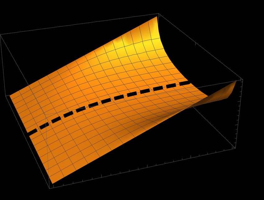
Contents

1 Introduction                                                                               1

2 Complexity of a Thermal Density Matrix                                                     3
  2.1 Two Mode Squeezing as Purification                                                     4
  2.2 Purification with Additional Ancillary Squeezing                                      10
  2.3 Complexity from Operator-State Mapping                                                13

3 Thermal Complexity in Curved Spacetimes                                                   16
  3.1 Complexity and Hawking Radiation                                                      17
  3.2 Complexity and Cosmological Perturbations                                             22

4 Discussion                                                                                28

A Complexity of Two-Mode Squeezing                                                          30

B Bogoliubov Transformations and Squeezed States                                            32

1   Introduction

The complexity of a quantum circuit, defined as the minimum number of unitary operations
that are needed to transform a given reference state into a particular target state [1–4], has
many interesting applications. There appear to be interesting connections to gravitational
holography, where the complexity of a field theory living on a boundary may characterize
features of its gravitational dual [5–7]. Quantum circuit complexity (hereafter simply referred
to as complexity) may also serve as a diagnostic for quantum chaos [8–10], and the complexity
of quantum cosmological perturbations shows interesting behaviors [11–13].
     While pure states are simple to work with, many interesting systems and phenomena are
described by mixed states, including decoherence and thermal states. A mixed state can be
transformed into a pure state through purification, in which the Hilbert space is enlarged to
include ancillary degrees of freedom such that the mixed state density matrix is recovered
as the trace of the pure state density matrix over the ancillary states. We will follow [14–
17] in defining the thermal complexity of purification as the minimum complexity of a set
of purifications of a thermal density matrix relative to the ground state. Alternatively, a
pure state can be associated to the density matrix through the technique of operator-state
mapping [18, 19], in such a way that the expectation values of observables are preserved. We
will consider both techniques in Section 2, finding that the extra freedom in scanning over

                                            –1–
ancillary states for the thermal complexity of purification leads to a smaller complexity (and
thus a more optimal unitary operator) than the unique pure state defined by the operator-
state mapping procedure.
We will focus on the thermal density matrix of a free harmonic oscillator, both for its
simplicity and because it can be directly related to several interesting applications. While
the thermal complexity of purification for this system has been studied before [15–17] (see
also [20, 21] for the entanglement of purification of similar systems), our analysis, based on
the approach of [4, 22], will include a somewhat more general purification as a two-mode
squeezed state with non-zero squeezing angle φ. Squeezed states can play an important role
in continuous variable quantum computing [23–27], and show up naturally in descriptions
of Hawking radiation and cosmological perturbations [28–31], among other applications. We
will find in Section 2.1 that the minimum thermal complexity of purification relative to the
ground state occurs at a non-zero squeezing angle, and saturates at high temperature T (or
√
low frequencies ω) to a constant Cth ≈ π/(2 2), as opposed to the complexity for a vanishing
squeezing angle that grows logarithmically with temperature Cφ=0 ∼ ln(T /ω). In Section 2.2,
we show that generalizing the purification further to also include single-mode squeezing of the
ancillary degrees of freedom introduces additional degeneracy in the purification parameters
for the minimized complexity, but does not change the value of the minimized complexity.
In Section 2.3, we show how the pure state obtained from operator-state mapping is a two-
mode squeezed state with a vanishing squeezing angle, and thus does not have a minimal
complexity. Altogether, we find that the two-mode squeezed complexity of purification with
a non-zero squeezing angle produces the simplest minimal complexity among these different
purification techniques.
We apply our results on the thermal complexity of purification to two interesting ap-
plications in quantum fields on curved spacetime where thermal density matrices can arise:
Hawking radiation and cosmological perturbation theory. In Section 3.1, we review how
Hawking radiation for a scalar field on a curved spacetime with horizons, such as Rindler
space or a black hole spacetime, can be described as a thermal state by tracing over a two-
mode squeezed state in which modes on either side of the horizon are entangled with each
other. We then illustrate how the optimal purification of complexity of this thermal state
takes the form of a squeezed state with a different squeezing angle and saturates at when
the effective temperature of the horizon is high, in contrast to the complexity of the original
squeezed state which grows with the effective temperature. While these are calculations of
complexity “in the bulk” (and are thus not directly related to holography), they may have
interesting implications for information-theoretic perspectives of black holes. In Section 3.2,
we review the application of the techniques of complexity to quantum cosmological pertur-
bations, such as those produced in the very early universe during inflation. Considering a
few simple models of decoherence, we show how the Fourier modes of these perturbations can
also be described by a thermal density matrix, and illustrate how the resulting saturation
of the thermal complexity of purification of the Universe compares before and after decoher-
ence. We conclude in Section 4 with a summary of our results and some speculation on their
–2–implications. Several appendices are included for reference and review.
2 Complexity of a Thermal Density Matrix
As discussed in the Introduction, we are interested in the complexity of a thermal state of a
quantum harmonic oscillator,
∞
1 X −βEn
ρ̂th = e |nihn| , (2.1)
Z
n=0
where En = ωn. In order to use established techniques [4, 22] to compute the complexity,
we need to represent the thermal state (2.1) as a pure state |Ψi. For any mixed state ρ̂mix
on the Hilbert space H, we can construct a purification of ρ̂mix which consists of a pure
state |Ψi in an enlarged Hilbert space Hpure = H ⊗ Hanc , where Hanc corresponds to an
“ancillary” set of degrees of freedom. If the trace of the density matrix of |Ψi over the
ancillary degrees of freedom gives the original mixed state Tranc (|ΨihΨ|) = ρ̂mix , we say that
|Ψi is a “purification” of ρ̂mix . Note that expectation
values of operators
acting in H are
preserved under purification, hÔi = Tranc hΨ|Ô|Ψi = Tr ρ̂mix Ô , so that observables are
preserved by purification.
Clearly, the purification |Ψi is not unique, since the choice of the ancillary Hilbert space
Hanc is arbitrary as long as it meets the purification requirement. For example, there may be
a set of pure states {|Ψiα,β,... }, parameterized by α, β, ..., all of which satisfy the purification
requirement. In order to distinguish among the set of purifications, it is often helpful to
minimize a quantity of interest, such as the entanglement entropy or complexity, with respect
to the parameters. In this work, we are interested in analyzing the complexity of the mixed
thermal state (2.1), so we will minimize the complexity of the set of purifications {|Ψiα,β,... }
of ρ̂th , obtaining the thermal complexity of purification
Cth (β) = min C (|Ψiα,β,... , |ψR i) , (2.2)
α,β,...
where we made explicit the dependence of the complexity of the pure state on the reference
state |ψR i.
We will choose three explicit purifications of ρ̂th (2.1). First, in Section 2.1 we will
purify ρth as a two-mode squeezed state, parameterized by a squeezing parameter r and
squeezing angle φ, in which the Hilbert spaces H, Hanc are entangled in such a way that a
trace over the ancillary degree of freedom gives rise to a thermal state. The corresponding
complexity of purification saturates as a function of inverse temperature. Next, in Section
2.2 we generalize the two-mode squeezed state purification to include additional squeezing
of the ancillary degree of freedom. We find that minimizing over the additional parameters
introduced by the extra squeezing provides more freedom in finding a minimum of (2.2), but
leaves the minimum value of the complexity of purification unchanged. Finally, in Section 2.3
we construct a purification of the thermal state through operator-state mapping.
–3–2.1 Two Mode Squeezing as Purification
A straightforward purification of the generic thermal state (2.1) is the thermofield double
state,
∞
1 X −βEn /2
|TFDi = √ e |ni ⊗ |nianc , (2.3)
Z n=0
where the ancillary Hilbert space Hanc is taken to be a copy of the original oscillator H.
However, the thermofield double state (2.3) is by no means unique as a purification of (2.1);
indeed, it is possible to include an additional phase, so that the purification |Ψiα,β... becomes
∞
1 X
|Ψiφ = |TFDiφ = √ (−1)n e−2inφ e−nβω/2 |ni ⊗ |nianc , (2.4)
Z n=0
where we took En = ωn for bosonic oscillators, and we introduced a factor of (−1)n (which
can be reabsorbed back into φ) for convenience. We recognize this as a two-mode squeezed
vacuum state,
∞
1 X
|Ψiφ = (−1)n e−2inφ tanhn r|ni ⊗ |nianc ≡ Ŝsq (r, φ)|0i ⊗ |0ianc , (2.5)
cosh r
n=0
where the squeezing parameter r is related to the oscillator frequency and temperature
through βω = − ln tanh2 r, and the squeezing angle φ is a free parameter; as part of the
purification of complexity process (2.2), we will minimize the complexity with respect to φ.
The operator Ŝsq (r, φ) is the two-mode squeezing operator, and is given in terms of raising
and lowering operators {â, ↠}, {âanc , â†anc } on the physical and ancillary oscillator Hilbert
spaces H, Hanc , respectively,
hr i
Ŝsq (r, φ) = exp e−2iφ ââanc − e2iφ ↠â†anc . (2.6)
2
The purification of the thermal state (2.1) into (2.5) is thus obtained by acting the squeeze
operator Ŝsq (r, φ) on the two-mode vacuum |0i ⊗ |0ianc . The two-mode squeezing operator
can be interpreted as a type of entanglement operator, as it mixes creation and annihilation
operators of the two Hilbert spaces H, Hanc
†
Ŝsq â Ŝsq = â cosh r − â†anc e2iφ sinh r ; (2.7)
† † 2iφ
Ŝsq âanc Ŝsq = âanc cosh r − â e sinh r . (2.8)
For the calculation of complexity1 , we are interested in the transformation of a reference
state |ψR i into a target state |ψT i
|ψT i = Û |ψR i (2.9)
1
See Appendix A for details.
–4–by a unitary operator Û representing the quantum circuit connecting these two states. Follow-
ing the geometric approach of [1–4], we decompose the unitary Û as a path-ordered sequence
of a set of fundamental operators {ÔI }
" ˆ #
sX
←
−
Û (s) = P exp −i Y I (s0 )ÔI ds0 . (2.10)
0 I
We define complexity in a geometric way as the circuit depth along a minimal path in the
geometry generated by the algebra of the operators
ˆ 1 sX
C= GIJ Y I Y J ds , (2.11)
0 I
where the Y I (s) are vectors that specify the path parameterized by s. To calculate the
complexity we follow [4, 11] in transforming our reference and target states into position-space
wavefunctions by defining the position variable q̂ = √12ω (↠+ â) (with a similar definition for
the ancillary variable q̂anc in terms of the âanc , â†anc ). Our reference state will be the (purified)
ground state |ψR i = |0i ⊗ |0ianc
1 2 2
hq, qanc |ψR i = NR exp − ω(q + qanc ) . (2.12)
2
Our target state is the purification (2.5), |ψT i = |Ψiφ , which also takes the form of a Gaussian
wavefunction
n ω o
Ψsq (q, qanc ) = hq, qanc |Ψiφ = N exp − A(q 2 + qanc 2
) − ωB q qanc (2.13)
2
where N is a normalization factor that will not be important here, and the squeezed Gaussian
parameters are
1 + e−4iφ tanh2 r 2 tanh r e−2iφ
A= , B= . (2.14)
1 − e−4iφ tanh2 r 1 − e−4iφ tanh2 r
Interestingly, the corresponding variances of the physical position q̂ and momentum p̂ =
i ω/2(↠− â) are independent of the squeezing angle
p
1
hq 2 i = cosh(2r) , hp2 i = ω cosh(2r) . (2.15)
ω
A curious feature of the two-mode squeezed state is that the uncertainty of the single oscillator
grows as the squeezing is increased hq 2 ihp2 i = cosh2 (2r), in contrast to a one-mode squeezed
state in which the uncertainty in one direction of phase space is reduced while the other
grows, preserving the total uncertainty2 . The growth in uncertainty of the single oscillator of
2
Two mode squeezed states do not preserve the total noise, but instead preserve the difference in the total
noises of the two modes. See [32] for other useful properties of two-mode squeezed states.
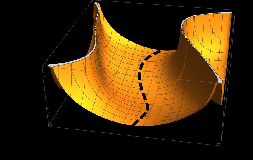
–5–Figure 1: Complexity (2.16) of the purified thermal state as a squeezed state, as a function of the squeezing
parameter r and the squeezing angle φ. The dashed line indicates the minimum of the complexity at φ = π/4. The
complexity saturates at large r (corresponding to high temperature) for generic φ as in (2.19), but grows linearly
with the squeezing r for the angles φ = 0, π/2.
the two-mode squeezed state mirrors the expected growth in uncertainty of a thermal state
with temperature, and is a desired property of our purification of the thermal mixed state.
The complexity (2.11) of the purified thermal state (2.13) thus becomes (see Appendix
A)
s
1 1 + e−2iφ tanh r
Cφ = √ ln2 + arctan2 (sin 2φ sinh 2r) (2.16)
2 1 − e−2iφ tanh r
s
−2iφ e−βω/2 e−βω/2
1 2 1+e 2
= √ ln + arctan 2 sin 2φ , (2.17)
2 1 − e−2iφ e−βω/2 1 − e−βω
where we substituted tanh r = e−βω/2 to make the temperature-dependence explicit. The
arctan contribution to the complexity is necessary when the parameters A, B of the Gaussian
wavefunction (2.13) take on complex values [22], and will play an important role in the
minimized complexity, as we will see.
Before we minimize the complexity (2.17) with respect to the squeezing angle φ as part
of the complexity of purification process (2.2), let us examine some of its useful limits. The
low-temperature limit βω → ∞ corresponds to vanishing squeezing r → 0; the system and
ancillary degrees of freedom are no longer entangled, as can be seen by the diagonalization
of the wavefunction (2.13) for A ≈ 1, B ≈ 0 in this limit. Correspondingly, the complexity
(2.17) vanishes as Cφ ∼ e−βω/2 at low temperatures βω
1, for all squeezing angles φ.
Alternatively, the high-temperature limit βω
1 corresponds to large squeezing r
1
in the squeezed-state language. For generic squeezing angles (specifically, for φ 6= nπ/2) the
–6–Gaussian wavefunction parameters (2.14) saturate to pure imaginary values at leading order
sin 4φ sin 2φ
A ≈ −i , B ≈ −2i . (2.18)
1 − cos 4φ 1 − cos 4φ
Thus, at high temperature (large squeezing), the two-mode squeezed state wavefunction (2.13)
is an approximately pure phase entanglement between the physical and ancillary degrees
of freedom. Correspondingly, the position variance diverges in the high-temperature limit
ωhq 2 i ∼ (βω)−1
1, consistent with the delocalization that is expected of a thermal state.
The saturation of the purified wavefunction to a pure phase at high temperatures leads to a
similar saturation of the complexity (2.17)
s
1 1 + cos 2φ π 2
Cφ ≈ √ ln2 + , (2.19)
2 1 − cos 2φ 2
which is independent of the temperature at leading order. The angle φ = π/4 is partic-
ularly interesting, since we see that the entangled Gaussian wavefunction becomes purely
off-diagonal in the high-temperature limit A ≈ 0, B ≈ i, and the complexity is minimal
√
Cφ/4 ≈ π/2 2.
The angles φ = nπ/2 are special cases, and lead to behaviors for the wavefunction and
complexity that are qualitatively different than the general case. For example, for a vanish-
ing squeezing angle φ = 0, the high-temperature limit corresponds to a strongly entangled
wavefunction with real Gaussian parameters A ∼ B ∼ (βω)−1
1. The corresponding com-
1 T
plexity (2.17) is then dominated by the first term Cφ=0 ≈ r ≈ ln βω = ln ω and grows
logarithmically with the temperature. The generic behavior of the complexity, as well as the
behavior for the special cases φ = nπ/2, can be seen in Figure 1.
We have purified the thermal state ρ̂th (2.1) into the two-mode squeezed state (2.5),
with corresponding complexity (2.17). The thermal complexity of purification (2.2)
is obtained by minimizing (2.17) over the squeezing angle φ, which we introduced as a free
parameter. The squeezed state complexity (2.17) is symmetric about π/4, and the complexity
is minimized at φ = π/4 for all values of the squeezing parameter r (or correspondingly, for
all values of the temperature βω) leading to
!
1 1 e−βω/2
Cth (β) = Cφ φ=π/4 = √ | arctan(sinh 2r)| = √ arctan 2 (2.20)
2 2 1 − e−βω
√
2 e−βω/2 low temperature limit βω
1
≈ π
(2.21)
√
2 2
high temperature limit, βω → 0
with the corresponding purification as a two-mode squeezed state with squeezing angle φ =
π/4
∞
1 X
|Ψith,p = |Ψiφ=π/4 = √ (−i)n e−nβω/2 |ni ⊗ |nianc . (2.22)
Z n=0
–7–C
3.0
Cϕ=0
2.5
2.0
1.5
π
1.0 Cϕ=π/4 2 2
0.5
T/ω
5 10 15 20
(a) Complexity of purification (2.17) as a function of (b) Thermal complexity of purification as a function of
temperature T = β −1 for φ = 0 and φ = π/4. the frequency ω for different fixed temperatures T .
Figure 2: The complexity of purification is minimized by the squeezing angle φ = π/4 and has the unique feature
√
that it saturates for high temperatures to Cφ=π/4 ≈ π/(2 2) ≈ 1.1, as seen in Figure 2a. For a fixed temperature
T , the minimal thermal complexity of purification Cth = Cφ=π/4 drops off sharply for high frequencies ω > T , as
seen in Figure 2b.
Interestingly, we find that the complexity of purification of the thermal density matrix ρ̂th
saturates at high temperature, as can also be seen in Figure 2. This saturation of the com-
plexity of the purified thermal density matrix with temperature is in contrast to previous
results [15], which did not include the squeezing angle in the process of purification, and
thus considered only real Gaussian wavefunctions. We see that purifying the thermal density
matrix to include a squeezing angle qualitatively changes the behavior of the complexity of
purification. As discussed above, the physical origin of this saturation is that at high temper-
ature the Gaussian wavefunction parameters (2.18) become imaginary and independent of the
temperature at leading order. The corresponding circuit depth saturates, even for arbitrarily
large temperature.
It is interesting to compare the thermal complexity of purification to the corresponding
entanglement entropy of the thermal state [33, 34]
e−βω
Ŝen = Tr [ρ̂th ln ρ̂th ] = − ln 1 − e−βω − ln e−βω
. (2.23)
1 − e−βω
The entanglement entropy of the thermal state is independent of the purification squeezing
angle φ, so that from the perspective of entanglement entropy, all two-mode squeezed states
that comprise the purification state (2.5) are equivalent, for any squeezing angle. However,
we have seen that complexity for building such states is not equivalent – it is in fact easier, by
a factor ∼ | ln(βω)|, to build the optimal purification state (2.22) ((2.5) with φ = π/4) than
it is to build the TFD state (2.3) ((2.5) with φ = 0), even though both of these states give
identical reduced thermal density matrices and have identical entanglement entropies (2.23).
This is in line with other observations that complexity is a more sensitive probe of a state
than entanglement alone [15, 35].
–8–Another interesting perspective of the thermal complexity of purification (2.20) is to
consider its dependence on the oscillator frequency ω for fixed temperature β = 1/T , as in
Figure 2b. For fixed temperature, the complexity drops off quickly as a function of frequency
Cth ∼ e−βω/2 , so that high frequency modes with ω > T contribute less to the complexity
than low frequency modes. The suppression of the complexity for purified high frequencies of
a thermal state characterizes the extent to which these modes are washed out by the thermal
background.
The thermal state of a single harmonic oscillator is easily generalizable
to a set of N
PN †
decoupled harmonic oscillators with Hamiltonian Ĥ = i=1 ωi âi âi + 1/2 , each of which
is in a thermal mixed state with individual thermal density matrix given by ρth (2.1). The
two-mode purification described above simply becomes a direct product of the individual
purifications, so that the total thermal complexity of purification for all the modes is the sum
v v
uN
−βωi /2 e−βωi /2
1 1
uX
N
uX
2 e 2
Cth = √ ≈√ t
u
t arctan 2 arctan 2 , (2.24)
2 1 − e−βωi 2 1 − e−βωi
i=1 ωiis a numerical constant. For example, for m = 0 and d = 1, I1 ≈ 3.7, the thermal complexity
of purification grows linearly with the temperature, while for m = 0 and d = 3, I3 ≈ 398,
the thermal complexity grows as the cube of the temperature. The temperature dependence
arises due to the density of states, since the complexity saturates for each mode with frequency
k < T in a sphere with radius set by the temperature.
We have considered the complexity of the purified target state (2.22) relative to the
ground state, but another natural candidate for a reference state is the factorized Gaussian
state [4, 15]
1 2 2
hq, qanc |ψf i = Nf exp − µ(q + qanc ) , (2.29)
2
where the reference frequency µ is the same for all oscillators and is not equal to the ground
state frequency ω. For a set of oscillators, this reference state is disentangled in the position
basis, so the complexity of the target state (2.22) relative to it is therefore a useful measure
of the difficulty in creating spatial entanglement. Minimizing the purified complexity with
respect to the squeezing angle, we now have an additional term in the thermal complexity of
purification
s
ω 2 e−βω/2
1 2
Cth,µ (β) = √ ln + arctan 2 . (2.30)
2 µ 1 − e−βω
For fixed temperature, the additional term ln |ω/µ| modifies the behavior of the complexity
at both high ω
µ and low frequencies ω
µ, reflecting the additional complexity needed
to establish spatial correlations in the target state (2.22).
2.2 Purification with Additional Ancillary Squeezing
A number of different purifications can be used to construct the complexity of purification
(2.2) since the minimization procedure scans over the ancillary parameters, while preserving
the reduced density matrix. Ideally, we wish to find the simplest purification that leads
the smallest complexity of purification of the thermal mixed state. We have already shown
that extending the purification of the thermal density matrix beyond that of a thermofield
double (2.3) to include a squeezing angle (2.4) qualitatively changes the value and functional
dependence of the complexity of purification on the temperature. However, it is possible to
generalize the purification further, and it is worth investigating whether including additional
ancillary parameters further changes the result in a qualitative way.
The purification of the thermal density matrix as a pure state consisting of a two-mode
squeezed state (2.5) can be generalized by the action of a two-mode rotation operator
|Ψiφ,θ = R̂(θ) Ŝsq (r, φ)|0i ⊗ |0ianc , (2.31)
where
h i
R̂(θ) = exp −iθ ↠â + â†anc âanc . (2.32)
– 10 –The rotation operator acts on the two-mode squeezed state as a shift φ → φ + θ and thus is
a redundant purification, so we can set θ = 0.
Because the ancillary degrees of freedom are traced out in the process of obtaining the
density matrix, we can perform additional transformations operating purely in Hanc . In
particular, we consider an additional single-mode squeezing of the ancillary oscillator by the
squeezing parameter and angle ranc , φanc
|Ψiφ,ranc ,φanc = Ŝanc (ranc , φanc ) Ŝsq (r, φ)|0i ⊗ |0ianc , (2.33)
where
h r i
anc
Ŝanc (ranc , φanc ) = exp − e−2iφanc â2anc − e2iφanc â†2
anc . (2.34)
2
We have now introduced two additional free parameters ranc , φanc , which will need to include
together with the two-mode squeezing angle φ in the minimization of the complexity (2.2).
This generalization is similar to the purification considered in [15], which also considered
an additional squeezing of the ancillary degrees of freedom (again, with vanishing squeezing
angle). However, because our two-mode purification mixes the physical and ancillary degrees
of freedom through the two-mode squeezing angle, in addition to having an additional pa-
rameter φanc , the calculation of the wavefunction and the minimization of the complexity
corresponding to (2.33) is somewhat more involved.
We can construct the position-space wavefunction corresponding to (2.33) as
Ψ(q, qanc )φ,ranc ,φanc = hq, qanc |Ψi = Sanc (ranc , φanc )Ψsq (q, qanc ) , (2.35)
where the single-mode ancillary squeeze operator in position-space takes the form
iranc
(qanc panc + panc qanc ) cos(2φanc ) + (ω −1 p2anc − ωqanc
2
Sanc = exp ) sin(2φanc ) (,2.36)
2
with panc = −i∂qanc . Using the auxiliary squeezing variables
iranc
v ≡ ranc cos 2φanc , u≡− sin 2φanc , (2.37)
2ω
and rewriting (2.36) using a BCH formula [36] as
ev −1 1−e−2v
u∂q2anc uω 2 qanc
2
Sanc = evqanc ∂qanc e v e 2v , (2.38)
the position-space wavefunction (2.35) takes the form
n ω ω o
Ψ(q, qanc )φ,ranc ,φanc = Ñ exp − Ãq 2 − Ãanc qanc2
− ω B̃qqanc . (2.39)
2 2
The Gaussian coefficients are
B2
à ≡ A − −1 , (2.40a)
A − (1 − e−2v ) uv + 2(ev − 1) uv
e2v
Ãanc ≡ −1 , (2.40b)
A − (1 − e−2v ) uv + 2(ev − 1) uv
Bev
B̃ ≡ . (2.40c)
1 + A − (1 − e−2v ) uv 2(ev − 1) uv
– 11 –Figure 3: The purification complexity (2.42) as a function of the squeezing angles (φ, φanc ) for βω = −2 ln tanh 50
and ancillary squeezing ranc = 1. The thick dashed line corresponds to the minimum as a function of (φ, φanc ),
tracing out a one-parameter curve in the valley of the complexity. In general, the minimized complexity of (2.42)
π
over the free purification parameters (φ, ranc , φanc ) is also a one-parameter curve, and approaches Cth ≈ 2√ 2
in the
high-temperature limit.
where A, B are as defined in (2.14). Notice that the wavefunction (2.39) has a similar Gaussian
form as (2.13), except now the coefficients of the physical position q 2 and ancillary position
2
qanc terms are no longer equal, as expected since we have performed an additional squeezing
of the ancillary oscillator. Notice that in the limit of vanishing ancillary squeezing ranc → 0,
the parameters reduce to their two-mode squeezing values Ã, Ãanc → A, B̃ → B, while in the
low-temperature limit βω
1, A → 1, B → 0 as before, so that the physical and ancillary
degrees of freedom decouple.
The wavefunction (2.39) is again Gaussian in form, and can be written in terms of the
normal mode frequencies
1
q
Ω± = 2
à + Ãanc ± (à − Ãanc ) + 4B̃ 2 . (2.41)
2
The corresponding complexity, including the ancillary squeezing, is then [4, 11]
s
1 Im Ω+ Im Ω−
Cφ,ranc ,φanc = ln2 |Ω+ | + ln2 |Ω− | + arctan2 + arctan2 . (2.42)
2 Re Ω+ Re Ω−
The thermal complexity of purification (2.2) is now the minimization of (2.42) over all
three parameters φ, ranc , φanc . Unfortunately, the expression is sufficiently complex that it is
difficult to do a purely analytic minimization. Instead, we note that in the high-temperature
– 12 –limit βω
1 the Gaussian parameters Ã, Ãanc , B̃ (2.40) and normal mode frequencies Ω±
(2.41) become purely imaginary. Further, we note that, as with the minimization of the
complexity arising from two-mode squeezing (2.17), the minimum of (2.42) occurs when the
ln |Ω± | terms vanish, which together requires Ω± = ±i. This becomes a condition on the
Gaussian parameters
1
à + Ãanc = 0 , (à − Ãanc )2 + B̃ 2 = −1 . (2.43)
4
For example, the first condition implies that the minima are found as solutions to the relation
ranc cot 2φanc
1 − e−2v tan 2φanc +
tan 2φanc + = 0. (2.44)
2 ranc (ev − 1)
Together, the conditions (2.43) impose two constraints on our three free parameters φ, ranc ,
and φanc , implying that generically there is a one-parameter set of minima. An example is
shown in Figure 3, where a valley of minimum complexity for ranc = 1 is found as a curve in
the (φ, φanc ) parameter space. The corresponding complexity, in the high-temperature limit,
is the same as for the two-mode squeezing
π
Cth = min Cφ,ranc ,φanc = √ . (2.45)
φ,ranc ,φanc 2 2
As discussed above, in the low-temperature limit βω
1 the physical and ancillary degrees
of freedom decouple, so the extra squeezing of the ancillary degrees of freedom becomes
irrelevant.
Altogether, we have found that generalizing the purification of the thermal density matrix
to include an additional squeezing of the ancillary degrees of freedom as in (2.33) leads to
the same minimized complexity of purification. In particular, the minimized complexity of
purification saturates to a constant value (2.45) at high temperature, and decays to zero at
low temperature. The additional degrees of freedom added lead to a one-parameter set of
such minima, as opposed to the single φ = π/4 minimized complexity of purification as with
the pure two-mode squeezing. Because the additional purification parameters ranc , φanc do
not change the value of the minimized complexity of purification, it seems that the additional
freedom (and difficult) arising from their addition is undesirable. However, there may be
situations where boundary conditions do not permit a squeezing angle φ = π/4, so that the
additional freedom of (2.44) is useful. Nevertheless, the conceptual picture that arises from
both the two-mode purification (2.13) and the additional ancillary squeezing (2.33) for the
thermal complexity of purification is the same: at low temperatures, the complexity vanishes
exponentially as a function of the inverse temperature, while it saturates at high temperature
to a constant value, becoming independent of the temperature.
2.3 Complexity from Operator-State Mapping
An alternative approach to assigning a pure state to the thermal density matrix ρ̂th (2.1)
is the technique of operator-state mapping (also known as channel-state mapping) [18, 19].
– 13 –Consider an operator on our physical oscillator Hilbert space H with representation Ô =
P
m,n Omn |nihm|. In its simplest form, the mapping associates a state |Oi to Ô by flipping
the bra to a ket,
X 1 X
Ô = Omn |nihm| ←→ |Oi = p Omn |mi ⊗ |nianc . (2.46)
m,n Tr[O† O] m,n
The state |Oi exists on the doubled Hilbert space H ⊗Hanc , where again we denoted the extra
copy of H as Hanc to distinguish it from the original. The process of operator-state mapping is
superficially similar to purification studied in the previous subsection, in that both associate
to the operator a state on a doubled Hilbert space. One of the most important differences,
however, is that the state |Oi in (2.46) associated to the operator Ô is unique – there are
no free parameters introduced in the mapping (indeed, this is essential for the mapping to
be an isomorphism) – as compared to the purification (2.4), which introduces a squeezing
angle φ that plays an important role in the minimization of the complexity. The complexity
associated with the operator-state mapping, in contrast, does not require a minimization over
parameters.
For the thermal density matrix (2.1) we can then directly associate to it the two-mode
squeezed state
∞
X 1 X
ρ̂th = 1 − e−βω e−nβω |nihn| ←→ |ρth i = 2 (tanh r)2n |ni ⊗ |nianc ,(2.47)
n
cosh r n=0
where tanh r = e−βω is the two-mode squeezing parameter written in terms of the temperature
as before. It is now straightforward to write |ρ̂th i in position space
(ω/π)1/2 ω
exp − A(r) q 2 + qanc
2
ρ(q, qanc ) = hq, qanc |ρth i = √ + ωB(r) q qanc , (2.48)
cosh 2r 2
where
1 + tanh4 r 2 tanh2 r
A(r) = , B(r) = . (2.49)
1 − tanh4 r 1 − tanh4 r
The corresponding operator-state thermal complexity of (2.47) relative to the ground
state now follows directly from Appendix A with a vanishing squeezing angle φ = 0
1 + tanh2 r 1 + e−βω
1 1
Cos [ρ̂th ] = √ ln = √ ln . (2.50)
2 1 − tanh2 r 2 1 − e−βω
For low-temperature βω
1,(2.50) vanishes as Cos [ρ̂th ] ∼ e−βω , while for high temperatures
βω → 0 the complexity grows as Cos [ρ̂th ] ∼ 2 ln(T /ω). The operator-state thermal complexity
(2.50) thus does not saturate at high temperatures, as compared to the thermal complexity of
purification (2.20). The reason is clear: the operator-state mapping (2.47) does not allow for
the inclusion of a squeezing angle, so the state |ρth i inherits a squeezing angle φ = 0 from the
thermal density matrix. The operator-state thermal complexity is not identical to the φ = 0
– 14 –complexity of purification (2.17), however, since a factor of tanh2 r appears in (2.47) instead
of a factor of tanh r, as in (2.5). This leads to a faster decay of the complexity Cos ∼ e−βω at
low-temperature as compared to the thermal complexity of purification.
An alternative method of computing the complexity of a mixed state density matrix such
as ρth is to work with the square root of the thermal density matrix ρ̂th as in [37], assigning
to it the state
1/2
X 1/2
|ρth i = ρth |ni ⊗ |nianc , (2.51)
nn
n
1/2 1/2 1/2
where ρth = hn|ρth |ni are the matrix elements of ρ̂th . The original operator is then
nn
obtained as a trace over the ancillary degrees of freedom; for example,
" #
h i X 1/2 1/2
1/2 1/2
ρ̂th = Tranc |ρth ihρth | = Tranc ρth ρth |nihm| ⊗ |nianc hm|anc (2.52)
nn mm
m,n
X
= (ρth )nn |nihn| . (2.53)
n
In order to calculate the complexity of the state (2.51), we again write it as a Gaussian
wavefunction in position-basis
ωα
1/2 1/2
q 2 + qanc
2
hq, qanc |ρth i = ρth (q, qanc ) = Ñ exp − + ωγ q qanc . (2.54)
2
where now
p
α = A(r) + B(r) , γ= 2B(r)(A(r) + B(r)) , (2.55)
and A(r), B(r) are the same functions of the squeezing parameter given in (2.48). It is
straightforward to see that α, γ reduce to the purification quantities A(r), B(r) with φ = 0
1/2
from (2.14), so that the operator-state complexity corresponding to the state ρ̂th relative to
the ground state reduces to
h i √
1/2
Cos ρ̂th = 2 arctanh e−βω/2 . (2.56)
h i
1/2
Thus, while the low-temperature behavior of Cos ρ̂th ∼ e−βω/2 matches that of the minimal
h i
1/2
complexity of purification, the high-temperature behavior Cos ρ̂th ∼ ln(T /ω) grows with
temperature, rather than saturating.
Figure 4 compares the results for the complexity of the thermal density matrix ρ̂th for
the different techniques we have used in this section: the minimal complexity of purification
Cth (2.20), the operator-state complexity associated with the density matrix Cos [ρ̂th ] (2.50),
and the operator-state complexity associated with the square root of the thermal density
1/2
matrix Cos [ρ̂th ] (2.56). Each technique gives a complexity that vanishes exponentially with
the temperature at low temperatures, while at high temperatures their behaviours differ: the
– 15 –Figure 4: A complexity can be associated with a mixed thermal density matrix ρ̂th through the complexity of purifi-
cation Cth (2.2), operator-state complexity of the density matrix Cos [ρ̂th ] (2.50), and the operator-state complexity
1/2
of the square root of the density density matrix Cos [ρ̂th ] (2.56). As also discussed in the previous section, the
complexity of purification saturates at high temperatures, while the operator-state complexities grow logarithmically
with temperature ∼ ln(T /ω).
minimal complexity of purification saturates at high temperatures, while the operator-state
complexities grow as ln(T /ω). Because of the latter behavior, the operator-state complexity
diverges in the infrared logarithmically with the IR cutoff.
1/2
Qualitatively, each of the states |Ψiφ (2.4), |ρth i (2.47) and |ρth i reproduce the thermal
expectation values in the physical Hilbert space when traced over the additional degrees
of freedom, so which complexity should we associate with the thermal density matrix ρ̂th ?
Viewing complexity as the minimization of the number of gates (“circuit depth”) needed
to construct the target state from a given reference state, the complexity of purification
allows us to construct a state, namely |Ψiφ=π/4 , that reproduces all of our physical observables
with a smaller number of gate resources than the other techniques. In contrast, because it
1/2
maps to a unique target state, the operator-state complexity for either ρ̂th or ρ̂th picks out a
unique path in state space, which has no particular reason to be minimal (and in fact we find
it is not minimal). Thus, from the perspective of resource management, the complexity of
purification allows us to simulate the mixed state as a pure state with a smaller number of
resources.
3 Thermal Complexity in Curved Spacetimes
In the previous section we have shown how the complexity for a thermal density matrix of
a harmonic oscillator can be obtained by calculating the complexity of a corresponding two-
mode squeezed state parameterized by a squeezing parameter (fixed by the temperature) and
a squeezing angle. Since the thermal density matrix is independent of the squeezing angle, we
minimized the complexity with respect to the squeezing angle and found that the minimum
complexity corresponds to a non-zero squeezing angle.
– 16 –The thermal density matrix of a harmonic oscillator arises as a simple model in many
different contexts; here, we would like to explore the complexity of thermal density matrices
that arise naturally when considering quantum fields on curved spacetimes.
3.1 Complexity and Hawking Radiation
Thermal density matrices naturally arise when considering quantum fields on spacetimes with
horizons through the Unruh effect and the generation of Hawking radiation, so these are ideal
backgrounds to consider applications of the thermal complexity of purification. See [38–43]
for some useful reviews.
As an illustrative example that contains most of the relevant details, let us begin by
considering (1+1)-dimensional Minkowski space as seen by a uniformly accelerating observer.
The metric can be written
ds2 = −dt2 + dx2 = −du dv = e2aξ (dτ 2 − dξ 2 ) , (3.1)
where u = t − x, v = t + x are Minkowski light-cone coordinates and (τ, ξ) defined by
1 aξ 1 aξ
t= e sinh(aτ ) , x= e cosh(aτ ) (3.2)
a a
are coordinates adapted to a uniformly accelerating observer with acceleration a along ξ = 0.
The coordinates (τ, ξ) in (3.2) only cover part of the original Minkowski space, the so-called
right R Rindler wedge |x| > t; a similar definition is needed, with additional minus signs,
for the L wedge. An interesting and important feature of Rindler coordinates is that u = 0
is a future horizon for an observer traveling along a constant ξ line in the R wedge (v = 0
is correspondingly a past horizon), so that the R and L patches are causally disconnected
from each other. See Figure 5a for a spacetime diagram of Minkowski space and R, L Rindler
wedges.
A massless scalar field φ on this spacetime can be expanded in Minkowski (t, x) plane
wave modes
X
M∗ †
φ̂ = uMk âk + uk âk (3.3)
k
where the Minkowski vacuum is defined by the annihilation operator âk |0iM = 0. We can
also expand the scalar field in modes adapted to Rindler (τ, ξ) coordinates
X
R∗ R† L∗ L†
φ̂ = vkR b̂R
k + v L L
b̂
k k + v k b̂k + v k b̂k (3.4)
k
where v̂kR,L are only non-zero in the R, L wedges, respectively, and the Rindler vacuum can be
written as the direct product of vacuum states on the left and right wedges |0iR ⊗ |0iL , which
are annihilated by the left- and right-Rindler annihilation operators, b̂R L
k |0iR = 0 = b̂k |0iL .
The Minkowski and Rindler vacuum states are not equivalent; instead, the Minkowski
vacuum of a single mode k of the scalar field φ as seen in the basis of Rindler modes (3.4)
– 17 –t
0
v τ = const
V
0
=
=
=
r = 0
=
u
0
U
0
ξ = const III
L R x
II I
IV
(a) Rindler spacetime split into R and L wedges. (b) Kruskal spacetime for a black hole.
Figure 5: Spacetime diagrams for Rindler and Kruskal spaces.
takes the form of an two-mode squeezed state entangling the L and R modes [41, 42], which
we will call the “Unruh” state
∞
1/2 X nπk
|0iM = 1 − e−2πk/a e− a |nk iR ⊗ |nk iL . (3.5)
nk =0
Comparing (3.5) with (2.5), the squeezing parameter is tanh r = e−πk/a with squeezing angle
φ = π/2. The corresponding complexity of this Unruh state relative to a Rindler ground
state |0iR ⊗ |0iL is
πk
!
1 1 + e− a
CUnruh (k) = √ ln πk , (3.6)
2 1 − e− a
and grows logarithmically CUnruh ∼ r ∼ ln(a/k) for large accelerations a/k
1. Interestingly,
the complexity (3.6) of the Unruh two-mode squeezed state is maximal with respect to the
squeezing angle – that is, for fixed acceleration, the squeezing angle of the squeezed state
(3.5) chooses the largest possible complexity. We will return to this observation at the end of
this section.
A Rindler observer in the R-wedge sees a density matrix with the unobservable L modes
traced out
X
ρ̂R = TrL [|0iM h0|M ] = 1 − e−2πk/a e−2πnk k/a |nk iR hnk |R , (3.7)
nk
which is identified as a thermal density matrix of Hawking radiation with temperature T =
a/2π. The thermal complexity of purification from Section 2.1 assigns a minimal purification
– 18 –to (3.7)
∞
1/2 X
πnk k
|ΨiHawk,p = 1 − e−2πk/a (−1)nk e−2ink φ e− a |nk iR ⊗ |nk iL0 , (3.8)
nk =0
with the same squeezing parameter r as with the Unruh state, but now with squeezing angle
φ = π/4 as determined by the minimization of the complexity of purification. Note that
the purification includes an ancillary Hilbert space, which we will denote as L0 due to its
similarity with the L wedge of Rindler space. Comparing the Unruh squeezed state (3.5)
and the purification of the Hawking radiation (3.8), these two purifications differ only by
the value of the squeezing angle φ: The Unruh squeezed state (3.5) has φ = π/2, which as
discussed in Section 2.1 maximizes the corresponding complexity for fixed acceleration, while
the minimization arising from the thermal complexity of purification selects φ = π/4. The
minimized complexity of purification for the Hawking thermal density matrix (3.7) is instead
!
1 e−πk/a
CHawk,p (k) = √ arctan 2 , (3.9)
2 1 − e−2πk/a
√
which saturates to CHawk,p ∼ π/(2 2) for large accelerations a/k
1. The minimization
imposed by the thermal complexity of purification leads to a different qualitative behavior of
the complexity of the Hawking radiation as a function of the acceleration, compared to the
complexity of the full Unruh squeezed state. Nevertheless, because the purification process
preserves expectation values, both purifications (3.5), (3.8) of the thermal density matrix
(3.7) are equivalent to an observer in the R wedge. Thus, a R wedge observer can reconstruct
thermal expectation values by using the purification (3.8), which is easier to build (in that it
has a smaller complexity) compared to the Unruh squeezed state (3.5).
The role of the squeezing angle arises in the analytic continuation of positive frequency
mode functions from the R wedge to the L wedge. To see this, we expand the global scalar
field in a set of different positive frequency mode functions in Minkowski space
X
I∗ I† II∗ II†
φ̂ = ŪkI ĉIk + ŪkII ĉII
k + Ūk ĉk + Ūk ĉk (3.10)
k
where the modes ŪkI , ŪkII are defined as combinations of the Rindler mode functions that have
positive frequency in Minkowski coordinates. This corresponds to a Bogoliubov transforma-
tion between the Minkowski modes ĉIk , ĉII R L
k and the Rindler modes b̂k , b̂k
v v
u πk u πk
I
u e a
R − πk L†
II
u ea
L − πk R†
ĉk = t b̂k + e a b̂k ; ĉk = t b̂k + e a b̂k . (3.11)
2 sinh πk 2 sinh πk
a a
πω
The factors of e− a arise from the analytic continuation of the positive frequency mode
functions from the R wedge to the L wedge, and give rise to the temperature as seen by an
R wedge Rindler observer.
– 19 –As reviewed in Appendix B, the Bogoliubov transformations (3.11) can be seen as a
special case of a two-mode squeezing transformation
v v
u πk u πk
I
u e a
R πk
2iφ − a L † 0
II
u ea 0
L 2iφ − πk R†
ĉk = t b̂k − e e b̂k ; ĉk = t b̂k − e e a b̂
k (3.12)
,
2 sinh πk 2 sinh πk
a a
with a squeezing angle φ = π/2 that ensures continuity of the ŪkI , ŪkII mode functions in
Minkowski space across the u = 0 = v boundary between the R and L wedges. Interpreting
the L0 wedge in a similar geometric way, an arbitrary squeezing angle φ for the purification
(3.8) would instead imply a phase discontinuity when crossing the Rindler horizon, which can
0 0
be absorbed in the Rindler mode function behind the horizon, vkL → vkL e2iφ . The minimized
squeezing angle φ = π/4 arising from the complexity of purification thus results in a purely
imaginary phase. It is interesting that this phase in the Bogoliubov transformations (3.12)
has qualitatively different effects on the complexity of the resulting squeezed state, and it
would be interesting to see whether this phase has any other physical effects.
Other spacetimes with horizons also exhibit the Unruh effect, for similar conceptual and
technical reasons. For example, consider a black hole spacetime, as shown in the Kruskal
diagram of Figure 5b. Ignoring the angular directions and treating spacetime as (1 + 1)-
dimensional, the metric is
2GM −1 2
2 2GM 2 2GM
ds = − 1 − dt + 1 − dr = − 1 − du dv
r r r
16G2 M 2 −r/2GM
=− e dU dV (3.13)
r
where we introduced the lightcone coordinates
u = t − r∗ = −4GM ln(−U/2GM ), v = t + r∗ = 4GM ln(V /2GM ) (3.14)
where r∗ = r + 2GM ln(r − 2GM ). A massless scalar field can be expanded in modes
X
φ̂ = uk âk + u∗k â†k (3.15)
k
X
I∗ I† II∗ II†
= vkI b̂Ik + vkII b̂II
k + vk b̂k + vk b̂k (3.16)
k
where the uk modes are defined with respect to the global (U, V ) coordinates and define the
vacuum in the asymptotic past âk |0ipast = 0, and the vkI,II modes are defined with respect to
the (u, v) coordinates in the I, II patches and define the vacuum seen by an observer outside
the black hole in the asymptotic future b̂Ik |0iI = 0 and the internal vacuum with respect to
the modes inside the black hole b̂IIk |0iII = 0. As in Rindler space, these modes are mixed by
a Bogoliubov transformation (again, see [38–43] for reviews), so that the past vacuum can be
– 20 –written as a squeezed state with φ = π/2, entangling the external and internal modes with
each other as an Unruh state
|0ipast = Nk exp e−4πGM k b̂I†
k kb̂II†
|0iI ⊗ |0iII
X
= Nk e−4πGM k nk |nk iI ⊗ |nk iII , (3.17)
nk
with corresponding complexity
1 + e−4πGM k
1
CUnruh (k) = √ ln . (3.18)
2 1 − e−4πGM k
As with Rindler space, the density matrix as seen by an external observer in the asymp-
totic future is obtained from (3.17) by tracing out the modes inside the horizon, leading to
a thermal density matrix with temperature TBH = (8πGM )−1 corresponding to Hawking
radiation of the scalar field φ. The corresponding thermal purification of complexity asso-
ciates a squeezed state to this density matrix, entangling the external modes associated with
I with ancillary degrees of freedom on a space II0 with squeezing angle φ = π/4, leading to
the purification complexity
e−4πGM k
1
CHawk,p (k) = √ arctan 2 , (3.19)
2 1 − e−8πGM k
As before, the complexity (3.19) associated with the purification of the thermal density matrix
is qualitatively different from that of the global Unruh state complexity (3.18), particularly
at low-frequencies or small masses, saturating instead of growing as GM k → 0.
We have reviewed how quantum field theory on curved spacetimes with a horizon natu-
rally leads to a Unruh two-mode squeezed state entangling degrees of freedom on either side
of the horizon through the Unruh effect, with an associated complexity. Interestingly, the
complexity of this Unruh squeezed state is maximal with respect to the squeezing angle.
In particular, the squeezing angle that naturally arises in the Bogoliubov transformation of
the Unruh state gives the largest complexity for a given squeezing, such that the complexity
grows with the squeezing CUnruh ∼ r, which itself is an increasing function of the acceleration
(for Rindler spacetimes) or the black hole mass. For a black hole, this agrees with expec-
tations from other work that black holes are maximally chaotic quantum systems [44–46],
and perhaps similar statements apply to Rindler space as well. It is therefore interesting to
speculate that the complexity for the Unruh black hole state is maximal because of some
deeper principle that applies more generally, which may take the form of a tendency for the
field configuration to maximize the complexity in a kind of second law of complexity, similar
to entropy. At least in our simple model of a scalar field on curved backgrounds, this seems
to be the case.
However, an observer outside the horizon sees a thermal density matrix of Hawking
radiation, obtained by tracing out over the internal modes. The thermal complexity of pu-
rification from Section 2 then associates an ancillary two-mode squeezed state description
– 21 –to the Hawking radiation. The purified Hawking radiation state takes a similar form as the
Unruh squeezed state, but with a squeezing angle that instead minimizes the complexity at
√
a constant value CHawk,p ∼ π/(2 2). This implies that for an observer outside of the hori-
zon, it is easier to build the Hawking radiation as a two-mode squeezed state entangling the
Hawking radiation with ancillary degrees of freedom at a particular squeezing angle φ = π/4
that differs from the Unruh state. For a black hole of mass M , the difference between the
maximal Unruh complexity and the minimal purification complexity for fixed frequency k
is only weakly dependent on the mass of the black hole, CUnruh /Cp ∼ ln(GM k). However,
including many frequencies k this effect can potentially become an important effect.
Finally, as discussed in Section 2.1, note that the Unruh state (3.5) and the purification
of the Hawking radiation (3.8) have identical entanglement entropies that only depend on the
temperature and frequency through βk
e−βk
Sen = ln 1 − e−βk − ln e −βk
. (3.20)
1 − e−βk
Thus, while there are several ways that an observer outside the horizon can construct a pure
state representing the Hawking radiation with identical entanglement entropies (parameter-
ized by different values of the squeezing angle φ), the purification (3.8) is minimal with respect
to the complexity of building the state, by a factor ∼ ln(GM k) compared to the usual Unruh
state (3.5) for black holes. It would be interesting to consider whether this difference has an
impact on the information contained in the Hawking radiation in a more robust treatment.
We leave these interesting questions for future work.
3.2 Complexity and Cosmological Perturbations
Squeezed states and thermal density matrices also arise in the quantum description of cosmo-
logical perturbations, in which the time-dependence of the metric induces the pair creation
of particles from the vacuum.
We will briefly review the description of cosmological perturbations as squeezed states;
see [11, 12, 28–31, 47] for more details. Our metric is the spatially flat Friedmann-Lemaitre-
Robertson-Walker (FLRW) metric
ds2 = −dt2 + a(t)2 d~x2 = a(η)2 −dη 2 + d~x2 .
(3.21)
The Hubble expansion rate of this background is denoted by H = ȧ/a, where a dot denotes
a derivative with respect to cosmic time t. On this background we will consider fluctuations
of a scalar field, which combine with fluctuations of the metric to form the gauge-invariant
curvature perturbation R. Written in terms of the Mukhanov-Sasaki variable v ≡ zR where
√
z ≡ a 2, with = −Ḣ/H 2 = 1 − H0 /H2 , the action takes the simple form
ˆ " 0 2 #
1 3 02 2 z 2 z0 0
S= dη d x v − (∂i v) + v −2 v v . (3.22)
2 z z
– 22 –You can also read


