Bio-Electromagnetics without Fields: The Effect of the Vector Potential - Scientific Research ...

Page created by Samuel Payne
 
CONTINUE READING
Bio-Electromagnetics without Fields: The Effect of the Vector Potential - Scientific Research ...
Open Journal of Biophysics, 2021, 11, 205-224
                                                                                              https://www.scirp.org/journal/ojbiphy
                                                                                                            ISSN Online: 2164-5396
                                                                                                              ISSN Print: 2164-5388

Bio-Electromagnetics without Fields:
The Effect of the Vector Potential

Andras Szasz

Biotechnics Department, St. Istvan University, Budaors, Hungary

How to cite this paper: Szasz, A. (2021)         Abstract
Bio-Electromagnetics without Fields: The
Effect of the Vector Potential. Open Journal     Numerous considerations deal with specialties of bioelectromagnetic effects,
of Biophysics, 11, 205-224.                      including the force-free and field-free interactions. The fact that bioelectro-
https://doi.org/10.4236/ojbiphy.2021.112007
                                                 magnetic phenomena consist of effects without mechanical forces and even
Received: March 18, 2021
                                                 without measurable fields looks impossible in the simple considerations.
Accepted: April 27, 2021                         However, the stochastic fluctuations cause surprising results, with scientifi-
Published: April 30, 2021                        cally proven bioelectromagnetism in field-free conditions. In the first steps,
                                                 we show the scalar and vector potentials’ specialties instead of electric and
Copyright © 2021 by author(s) and
Scientific Research Publishing Inc.
                                                 magnetic fields defined by the well-known Maxwellian equations. The va-
This work is licensed under the Creative         nishing of the fields is connected to the potentials’ stochastic fluctuations, the
Commons Attribution International                noises control the “zero-ground”. The result shows a possibility of a wave that
License (CC BY 4.0).
                                                 has no attenuation during its transmission through the material. In this
http://creativecommons.org/licenses/by/4.0/
                                                 meaning, the result is similar to the consequences of the scalar-wave (SW)
                Open Access
                                                 considerations. The structural changes follow a particular noise spectrum
                                                 (called pink-noise or 1/f noise), which keeps the entropy constant in a broad
                                                 range of scaling magnification.

                                                 Keywords
                                                 Vector-Potential, Scalar-Potential, Stochastic-Processes, Field-Free Effects,
                                                 Curl-Free Fields, Axial-Vector, Life, Homeostasis, Entropy, 1/f Noise

                                               1. Introduction
                                               The scientific research on electromagnetic effects on biological systems involves
                                               numerous theoretical and practical aspects in the last couple of centuries. Elec-
                                               tric and magnetic fields, depending on their intensity, frequency, and gradients,
                                               affect the biological processes, including the immune cells [1]. The magnetic
                                               field could support chemotherapy in oncology [2], despite missing observable
                                               clinical changes, the improvement of the patients’ quality of life is expected. On

DOI: 10.4236/ojbiphy.2021.112007          Apr. 30, 2021            205                                   Open Journal of Biophysics
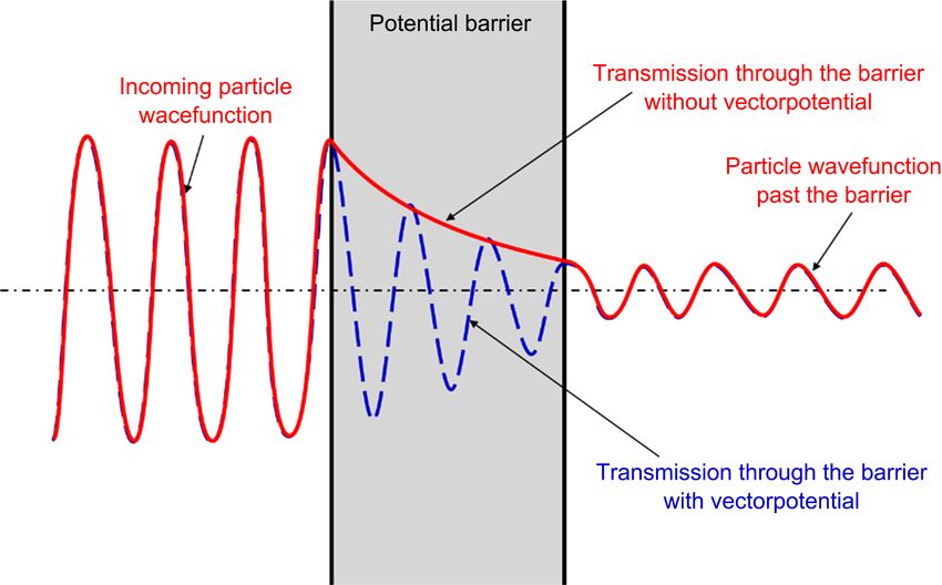
Bio-Electromagnetics without Fields: The Effect of the Vector Potential - Scientific Research ...
A. Szasz

                                   the other hand, the current research shows the active role of the magnetic vector
                                   potential in biological processes [3]. The effect of weak magnetic fields is fre-
                                   quently described with a vector potential in several biological studies of [4] [5].
                                   The vector potential can modify the quantum-states of the water [6], which
                                   could modify the complete chain-processes in living objects, governed by the
                                   phosphorylation catalyzing metal ions with magnetic nuclei [7].
                                      Alternative medicine frequently uses the idea of water-state modification con-
                                   siderations [8], sometimes applying unproven effects. Controversial discussions
                                   about the “silent” bioelectromagnetics as “energy-medicine”, [9] with force-free
                                   action on the viability of bacteria E. coli [10], the “electrosmog” [11] [12], the
                                   “new biophysical field”, “force-free actions” [13], “scalar-wave effects” [14],
                                   “subtle energies” [15] generate heated debates. Intense debates with opposing
                                   opinion on physical [16] and mathematical basis [17] [18] for evidence-less ap-
                                   plications were published. Direct investigation of quackery [19] and the variants
                                   of electromagnetic methods are questioned [20] [21]. Despite some spectacular
                                   results of the magnetic therapies, solid scientific proof and clinical evidence are
                                   missing, but the public’s hopes keep alive even the poorly documented cases.
                                   The weak proofs well support the medical skepticism [22] [23].
                                      The famous Maxwell equations [24] base the classical electrodynamics. Max-
                                   well revolutionary introduced new physical quantities: the electric (  ) and the
                                   magnetic (  ) fields. The standing (free charge density ρ ) and moving (cur-
                                   rent density j ) charges in vacuum form the sources of the fields:
                                                                        1
                                                          div (  ) =        ρ and div (  ) = 0                          (1)
                                                                        ε0
                                   and the sources of the field’s whirls in vacuum:
                                                                     ∂                         ∂
                                                     rot (  ) = −       and rot (  )= j + ε 0                           (2)
                                                                      ∂t                        ∂t
                                   where ε 0 ≅ 8.854 × 10⁻¹² F m is a universal constant.
                                     The conservation law of the charge:
                                                                        ∂ρ
                                                                           + div ( j ) =
                                                                                       0                                  (3)
                                                                        ∂t
                                      Sources and whirls define a vector-field which mathematical scheme makes
                                   the Maxwell Equations (1)-(2) complete to determine the two field-vectors 
                                   and  . In presence of materials (like living objects, too), we have to take into
                                   account the atomic and molecular structures, which have bounded charges. In
                                   the case of the presence of materials, new sources appear. Introducing the elec-
                                   tric-(P) and magnetic-(M) polarization vectors, we get the electric displacement
                                   field (D) and the magnetic induction (B):
                                                          =             B µ0  + M
                                                          D ε 0 + P and=                                                 (4)

                                   and µ0 ≅ 1.256 × 10⁻⁶ N A 2 , is a universal constant.
                                     Generally, we assume P and M depend on the  and B fields respectively, so
                                   their Taylor’s series:

DOI: 10.4236/ojbiphy.2021.112007                        206                                        Open Journal of Biophysics
A. Szasz

                                                                                  1  ∂2 P   1  ∂3 P 
                                   P ( )
                                   =            ( P ( ) ) =0 +  ∂∂P      +  2   2 +  3   3 + ⋅⋅⋅
                                                                                  2  ∂  0=6  ∂  0
                                                                         ==
                                                                             0

                                         and
                                                                          ∂M            1  ∂2 M                                (5)
                                     M(
                                                 ( M ( ) )=0 + 
                                               ) =                                   +       
                                                                                                             2

                                                                         ∂ =0        2  ∂2 =0
                                                   1  ∂3 M 
                                                  +           3 + ⋅⋅⋅
                                                   6  ∂3 =0

                                     The practical engineering simplifies (5) by considering only the linear term:
                                                              ∂P                                    ∂M
                                                                                                       
                                                    P ( ) =         and M (                   ) =
                                                                                                                                (6)
                                                              ∂  = 0                             ∂  = 0
                                   consequently
                                                                     1  ∂P  
                                                             ε 0 1 +     =
                                                            D=                        ε 0ε r  and
                                                                    ε 0  ∂  =0 
                                                                                                                                  (7)
                                                                   1  ∂M  
                                                             µ0 1 + 
                                                            B=                                  µ0 µ r
                                                                                                   =
                                                                                                   
                                                                 µ0  ∂ =0 
                                   where ε r and µr (relative permittivity and relative permeability, respectively)
                                   denote the material parameters, which are constant in the linear approach. The
                                   linearity requests very special conditions: homogeneous materials, adequately
                                   small fields, and no permanent/remnant polarization/magnetization, and addi-
                                   tionally the P (  ) and M (  ) functions must be smoothly continuous (ex-
                                   isting derivatives are necessary).

                                   2. Bio-Electromagnetism
                                   First, confirm that you have the correct template for your paper size. The living
                                   material is inherently highly polarized and extremely heterogeneous and has
                                   various non-linear processes (physiological feedback). The linear approach does
                                   not describe the real, heterogeneous, non-linear living phenomena. The correct
                                   formulation of the complete Maxwell equations for living matter uses (4):
                                                                                     ρ
                                                                                )
                                                                         div ( =       − div ( P )                               (8)
                                                                                     ε0
                                                                               div ( B ) = 0                                      (9)

                                                                                              ∂B
                                                                              rot (  ) = −                                     (10)
                                                                                              ∂t
                                                                                     ∂      ∂P
                                                         rot ( B ) =µ0 j + µ0ε 0        + µ0    + µ0 rot ( M )                  (11)
                                                                                     ∂t      ∂t
                                     Define the effective sources by comparison (1)-(2) with (8)-(11):
                                                                          ρeff= ρ − ε 0 div ( P )                               (12)
                                   and
                                                                                    ∂P
                                                                        jeff =j +      + rot ( M )                              (13)
                                                                                    ∂t

DOI: 10.4236/ojbiphy.2021.112007                            207                                            Open Journal of Biophysics
A. Szasz

                                     Instead of the free-charge conservation (3) effective charge considering the
                                   presence of the material makes connection between the effective values:
                                                                 ∂ρeff
                                                                         + div ( jeff ) =
                                                                                        Ceff                        (14)
                                                                   ∂t

                                   where Ceff depends on the derivatives of the P and M vectors. When the de-
                                   rivatives vanish, the free-charge conservation (see (3)) remains in force, Ceff = 0 .
                                   The zero divergence in (9) (source-less condition because of magnetic monopole
                                   does not exist) defines a new quantity by introducing a vector-field ( A , called
                                   magnetic vector potential)
                                                                         B = rot ( A )                              (15)

                                   which automatically satisfies (9), because of div ( rot ( A ) ) ≡ 0 . The induction
                                   flux Ф of an open surface S, defines the physical meaning of the vector potential
                                   A having special role in bio-systems [25]. The Stokes’ theorem gives the induc-
                                   tion flux (Ф) encircled by the curve
                                                        =Φ        BdS ∫ rot ( A
                                                                ∫S=           = ) dS ∫L Adr                         (16)
                                                                       S

                                   where, the L circumflex of open surface S. Therefore, in the closed contour-line
                                   integral of vector potential gives Ф. On the one hand, the magnetic flux density
                                   in accordance with Faraday’s induction law (10) generates Eddy-current loops of
                                     . Let us enter the relationship using (15) and (10):
                                                                             ∂A 
                                                                    rot   +    =0                                (17)
                                                                             ∂t 
                                   which obviously introduces the ϕ scalar potential:

                                                                     ∂A 
                                                                  +    =− grad (ϕ )                              (18)
                                                                     ∂t 

                                     To define the scale of the potentials, we usually fix the divA by the Lorentz
                                   condition:
                                                                                   ∂ϕ
                                                                   divA + ε 0 µ0      =
                                                                                      0                             (19)
                                                                                   ∂t
                                     The wave equations of the potentials:
                                                                            ∂2 A
                                                                 ∆A − ε 0 µ0     =µ0 jeff
                                                                            ∂t 2
                                                                                                                    (20)
                                                                            ∂ 2ϕ   ρeff
                                                                 ∆ϕ − ε 0 µ0 2 =−
                                                                            ∂t      ε0
                                      The simple realization of “pure” A vector is the space outside of an infinite
                                   cylindrical solenoid with r0 radius supplied by I current in n loops creates
                                   the situation of A ≠ 0 when  = 0 and B = 0 , when the distance (d) from
                                   the solenoid d ′′r0 . In this case A has only azimuthal component ( Aθ ) in the
                                   entire space from d distance. Inside the coil, we have, of course, the well-known
                                    rot ( B=
                                           ) B=z 4πε 0 µ0 nI .

DOI: 10.4236/ojbiphy.2021.112007                        208                                    Open Journal of Biophysics
A. Szasz

                                         The basic effects of the vector potential A in the quantum-mechanical processes
                                      indeed had been shown experimentally by the Aharonov-Bohm (AB) effect [26].
                                      The A potential was directly verified pursuant to Equation (16). According to
                                      another experiment [27], the interference image shifts as compared to the free of
                                      the current case if the coil current is not equal to zero. The vector-potential A is
                                      a phase-shifter of the de Broglie-waves [28], measured experimentally too [29]
                                      Figure 1.
                                         The minimal value of A2 has physical meaning [30], measures the existence
                                      (change) of the topologic structures. It could be connected to a phase transition
                                      in quantum-chromodynamics too [31]. Despite the AB effect has a quantum
                                      (microscopic) nature, some AB observations are macroscopic presenting their
                                      theoretical and practical proofs.
                                         The two potentials (A and ϕ ) determine the full field picture by simple
                                      mathematical transformations, so instead of the six variables (two vectors 
                                      and  ), only four parameters (A is a vector and ϕ , is scalar) describes the
                                      complete electromagnetic phenomenon [32]. The potentials are not only aux-
                                      iliary quantities, presented as the basis of the description of electromagnetism
                                      [32]. The conservation of electric charge in (3) and (14) was considered as a
                                      fundamental condition instead of the induction law (10). The potential Equa-
                                      tion (18) was used [32]. In this approach, a variation principle derives from
                                      the above equations and the Maxwell theory. Interestingly the opposite
                                      process, from [32] from Maxwell equations, does not work. In the relativistic
                                      four-dimensional curved space-time the basis of the electrodynamic discussions
                                      is the four-dimensional potential vector, composed from the components of A
                                      and ϕ [33] [34].

                    Figure 1. Effect of vectorpotential on the electron’s eigenfunction, and the interference pattern. The shift is
                    created by the presence of vectorpotential (Aharonov-Bohm effect).

DOI: 10.4236/ojbiphy.2021.112007                             209                                       Open Journal of Biophysics
A. Szasz

                                   3. Electromagnetic Forces
                                   The fields are senseless for humans. A transformation to mechanical or high
                                   frequencies optical form must be involved to sense the electromagnetic activity.
                                   The optical frequencies present the fields in radiative waveforms, so presently,
                                   we deal with the force-transformation in invisible lower frequencies. Lorentz
                                   force density ( f ) [35] connects the fields with the classical “force-based”, hu-
                                   man mechanical sensing:
                                                                      f = ρ  + j × µ0                                    (21)

                                     In the existence of materials, when P and/or M are presented (this is the real
                                   case) ρeff and jeff have to be applied in the Lorentz force:
                                                                     f = ρeff  + jeff × B                                 (22)

                                     The trivial force-free solution is when fields vanish. (See below the “field-free”
                                   solution.) The other, non-trivial vanish of the force is [36] when
                                                                 ρ  ′′ j × µ0 
                                                                               and j ||                                   (23)

                                     Formulate it with the polarization terms [37]:
                                                                                      ∂P          ∂M         
                                           f = ρ  + j × B + ( P ∇ )  + ( M ∇ ) B +  µ0    × B  −  µ0    ×           (24)
                                                                                         ∂t            ∂t    
                                      The complex force of (24) contains the direct forces, the dipole interactions
                                   ( f dipole ), and the radiation pressure ( f rad ) by two-two terms, respectively:
                                                                =
                                                                f dipole   ( P∇ )  + ( M ∇ ) B                            (25)

                                                                   ∂P        ∂M         
                                                              =  µ0
                                                            f rad       × B  −  µ0    ×                                (26)
                                                                    ∂t            ∂t    
                                     These terms do not annihilate by (23) conditions. In consequence, the non-trivial
                                   solution of the force-field condition does not exist in bio-matter.
                                     The potential formulation of the Lorentz force density by potentials (15) and
                                   (18) in the formulae (24):
                                                ∂A                                           ∂A             
                                        f =− ρ      + grad (ϕ )  + j × rot ( A ) − ( P ∇ )      + grad (ϕ ) 
                                                ∂t                                           ∂t             
                                                                                                                           (27)
                                                                  ∂P                  ∂M  ∂A                     
                                           + ( M ∇ ) rot ( A ) +  µ0    × rot ( A )  +  µ0      ×    + grad (ϕ )  
                                                                     ∂t                      ∂t  ∂t              
                                      The dynamics of charged particles could also be introduced in parallel of the
                                   classical dynamics an equation [38].
                                                      d       q 
                                                          pe +=A  q ( v∇ ) A + q ⋅ v × rotA − q∇ϕ                        (28)
                                                      dt      c 
                                   where q is the electric charge. In more symmetric form:
                                                          d       q           1          
                                                                        −q∇  ϕ − ( v ⋅ A ) 
                                                              pe + A  =                                                  (29)
                                                          dt      c           c          
                                    The Equation (29) shows important behaviors of the potentials: eA is a
                                   momentum-like term, while ( v ⋅ A ) together with ϕ has potential character.

DOI: 10.4236/ojbiphy.2021.112007                          210                                        Open Journal of Biophysics
A. Szasz

                                   4. Tunneling through a Potential Barrier
                                   There is no Lorentz force acting in the direction of the charge velocity, so no
                                   energy exchange could happen. The probability pi of an energy-state Ei is
                                   proportional with the Boltzmann expression:
                                                                                       E
                                                                                      − i
                                                                           pi ~ e      kT
                                                                                                                            (30)

                                   does not change by (curl-free) magnetic action in particle-description. In prin-
                                   ciple, we expect an effect of the curl-free field [39], on the basis of quantum me-
                                   chanics.
                                      The quantum-mechanics derives the surface and bulk chemical reactions go-
                                   verning the living processes. The Schrödinger picture of quantum mechanics in
                                   a case when a particle of charge q moves in the electromagnetic field can be de-
                                   scribed by the time-dependent single-particle equation with Ψ wave-function
                                   and      Hamilton operator ignoring the reaction of a particle to the field:
                                                                              ∂Ψ
                                                                         i       =     Ψ                                   (31)
                                                                               ∂t

                                      The information obtainable about the system is given by the wave function Ψ
                                   normalized to one. Consequently, the phase of wave function includes all infor-
                                   mation relating to the system. It was shown by Aharonov and Bohm in their
                                   famous effect [40] that the potentials have a fundamental role in quan-
                                   tum-mechanics without using the electromagnetic fields. Schrödinger equation
                                   where Ψ ( r ,t ) is the complex wave function      is a Hamilton operator, de-
                                   scribing the total energy of the system, which, in the case of Aharonov-Bohm
                                   conditions [40], can be expressed as follows:
                                                                                            2
                                                                       1        
                                                                 =        ∇ − qA  + qϕ .                                  (32)
                                                                      2m  i      
                                   where q is the charge in the V volume
                                                                         q = ∫ ρ dr 3                                       (33)
                                                                                 V

                                     Consequently, the Schrödinger equation of (31):
                                                           ∂Ψ
                                                                                        2
                                                                  1        
                                                      i       =     ∇ − qA  Ψ + qϕΨ=                    Ψ                (34)
                                                            ∂t   2m  i      
                                     In Equation (34) only the potentials have a role; the classical fields are com-
                                   pletely missing. The scalar potential affects the potential energy, while the vector
                                   potential is connected to the charge’s momentum in the Schrodinger equation.
                                   In the plane-wave solution
                                                                               E ⋅ t − ( pm + qA ) r 
                                                           Ψ ( r , t ) ∝ exp  i                                         (35)
                                                                                          h           
                                    Note classical fields do not appear in Equation (34) too. Where pm is the
                                   mechanical momentum of the particle with m mass and v speed:
                                                                          pm= m ⋅ v                                         (36)

DOI: 10.4236/ojbiphy.2021.112007                        211                                            Open Journal of Biophysics
A. Szasz

                                     In consequence of (35), the magnetic vector-potential changes the wave-number
                                   only. Using the normality of Ψ

                                                              ∫V , r →∞ Ψ ( r , t ) Ψ ( r , t ) dV =                     (37)
                                                                                     *
                                                                                                   1

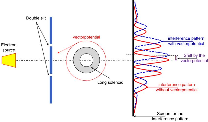
                                   and using (35) the coordination dependence of Ψ is:
                                                               1      p r       qA r 
                                                                 exp  − r  exp  −i r                                 (38)
                                                               r      h            h 

                                   which changes the amplitude of the wave-function at the transmission of a
                                   potential-barrier (Figure 2). The amplitude of the probability could be higher
                                   and also less under the action of the vector potential than without it.
                                     Consequently, when two charged particles create a chemical bond, the exter-
                                   nal vector-potential interacts and changes the structure.
                                     The average of effective sources jeff and ρeff could be expressed by:
                                                 =jeff  =
                                                       Tr [ j ] , ρeff Tr [ ρ                   ]                        (39)

                                   where      is the Neumann’s density operator:
                                                              ∂
                                                                 = − [        ], [   =Ψ  Ψ ]
                                                                    j     ,                                              (40)
                                                              ∂t    

                                     This approach (in principle) makes the complex system completely calculable.

                                   5. The “Curl-Free” Potential Situation
                                   A challenge arises when we have a curl-free magnetic vector potential:
                                                                       rot ( A ) = 0 ,                                   (41)

                                     In this case, (according to (15)) the B field vanishes, pure A field exists only
                                   [41]. A kind of the curl-free solution is free from the magnetic field, but accord-
                                   ing to (11) at high frequencies:

                                   Figure 2. Particle transmission through a potential barrier with and without magnetic
                                   vector potential.

DOI: 10.4236/ojbiphy.2021.112007                        212                                         Open Journal of Biophysics
A. Szasz

                                                                         rot ( B ) ≈ 0                                    (42)

                                   because from (11) a part could be zero, and the other part near to zero:
                                                                                            ∂      ∂P
                                                  µ0 j + µ0 rot ( M ) =
                                                                      0 and µ0ε 0              + µ0    ≈0                 (43)
                                                                                            ∂t      ∂t
                                     The electric field does not vanish if A changes by time ( A = A ( t ) ):
                                                                                       ∂A
                                                                   − grad (ϕ ) −
                                                                  =                      ≠0                              (44)
                                                                                       ∂t
                                      Of course, the curl-free solution could have bio-interactions having electric
                                   field and through this direct forces and energy absorption in the material. Using
                                   the potentials and the material parameters effective values of the sources ( ρeff
                                   and jeff ) can be introduced by potentials alone in case of (41) conditions, too:

                                                                 ∂P               1              ∂2 A 
                                                    jeff = j +      + rot ( M ) =     ∆A − ε 0 µ0 2                     (45)
                                                                 ∂t               µ0             ∂t 

                                   and
                                                                                                  ∂ 2ϕ 
                                                     ρeff =ρ − ε 0 div ( P ) =−ε 0  ∆ϕ − ε 0 µ0                         (46)
                                                                                                  ∂t 2 

                                     The time-dependent curl-free solution is a solution in the “pure”  -field,
                                   which is the most common in the literature, and mistakenly used as field free.
                                   The entire free field solution requests the following conditions:
                                                           ∂A
                                                              = 0 and grad (ϕ ) = const.                                  (47)
                                                           ∂t
                                     Note due to (41) a χ scalar-potential could be introduced:
                                                                      A = − grad ( χ )                                    (48)

                                   and so
                                                         ∂A                     ∂χ
                                                                     ) grad  − + ϕ= 0
                                                            + grad (ϕ=                                                    (49)
                                                         ∂t                   ∂t     
                                     Consequently, due to (18) the new scalar potential is time-dependent, as:
                                                                                       ∂χ
                                                                      ϕ ′ (t ) ⇒ ϕ −                                      (50)
                                                                                       ∂t

                                   6. “Field-Free” Solution
                                   The important question is the real field-free solution, when nor  nor B exist.
                                                                                                   ∂A
                                               =   =
                                                B rot               − grad (φ ) −
                                                      ( A ) 0 and  =                                 =
                                                                                                      0                   (51)
                                                                                                   ∂t
                                      The field-free solution does not mean that the space is also potential free.
                                   Could it interact with the biomatter?
                                      The field-free condition involves a full annihilation of the existing but identic-
                                   al and opposite fields. Due to the opposite ponderomotoric forces, the fields will

DOI: 10.4236/ojbiphy.2021.112007                         213                                         Open Journal of Biophysics
A. Szasz

                                   vanish from the system. The zero B could be described by the two oppositely ef-
                                   fective (destructive interference) vector potentials A and A :
                                                                               (
                                                                   B= rot A − A = 0           )                                    (52)

                                     In consequence, we could have a U scalar potential due to rot ( A ) = 0 for
                                   the difference A0
                                                                       (
                                                          A0 = A − A =grad (U )       )                    (53)

                                     Let us choose at the same time the scalar potential on the way that  has
                                   zero value as well:
                                                                            ∂ A − A           (          )
                                                       =  − grad ϕ − ϕ * −(   ∂t
                                                                                      =)0                  (54)

                                     In this case, using (52) we define:
                                                                                                   ∂U
                                                                    ϕ0 =(ϕ − ϕ * ) =                                                (55)
                                                                                                    ∂t
                                      Similarly to (20), the wave equations of these potentials belong to the
                                   field-free (source-free) conditions. In consequence of (45) and (46), the waves of
                                   null-potentials have zero effective charge- and current-densities
                                                                           (
                                                     jeff ( A, ϕ ) + jeff − A=
                                                                              , −ϕ * )
                                                                                     jeff ( A
                                                                                            =0 , ϕ0 ) 0
                                                                                                                                    (56)
                                                    ρeff ( A, ϕ ) + ρeff        , −ϕ )
                                                                           ( − A=         *
                                                                                                          A0 , ϕ0 ) 0
                                                                                                    ρeff (=

                                     The sum is zero in the macroscopic view. However, it does not automatically
                                   make terms vanish, the terms could be non-zero in a microscopic view! In this
                                   way, the potentials associated with null-fields appear as waves:
                                                                           ∂ 2 A0
                                                               ∆A0 − ε 0 µ0     = µ0 jeff
                                                                                      = 0
                                                                            ∂t 2
                                                                                                                                    (57)
                                                                           ∂ 2ϕ     ρeff
                                                               ∆ϕ0 − ε 0 µ0 20 =  −       =0
                                                                            ∂t      ε0

                                     There is a huge challenge: the waves of potentials in field-free solutions have
                                   no dumping. In consequence of the zero-field conditions, a U scalar potential in
                                   (53) and (55) is the potentials’ generator-function. Using (19), (52) and (54), a
                                   wave-equation is obtained for U:
                                                                                           ∂ 2U
                                                                      ∆U − ε 0 µ0               =0                                  (58)
                                                                                           ∂t 2
                                     The result in (58) supports the propagation of the scalar-wave (SW), which
                                   has no energy-dissipation in its transmission in the material [42]. The conse-
                                   quence of the SW concept, the Lorentz condition in (19) has been modified:
                                                                                           ∂ϕ
                                                                     divA + ε 0 µ0            =
                                                                                              C                                     (59)
                                                                                           ∂t
                                   where C ≠ 0 constant, and followingly [43]:
                                                                       ∂ 2C     ∂ρ          
                                                            ∆C − ε 0 µ0 =    µ  + div ( j )                                       (60)
                                                                        ∂t 2    ∂t          

DOI: 10.4236/ojbiphy.2021.112007                        214                                                    Open Journal of Biophysics
A. Szasz

                                     Due to the charge conservation rule (3):
                                                                     ∂ρ             
                                                                        + div ( j )  =
                                                                                       0                                    (61)
                                                                     ∂t             
                                     Consequently:
                                                                                   ∂ 2C
                                                                   ∆C − ε 0 µ0          =0                                  (62)
                                                                                   ∂t 2
                                   Which is equal with (58).
                                    Due to
                                                                                   1
                                                                        ε 0 µ0 =                                            (63)
                                                                                   c2
                                     These null-potential waves (together with the wave of the U potential (58)),
                                   are traveling by the speed of light in the vacuum (c), and so there are not dump-
                                   ing. [Note the limited velocity (c) of null-field potential obtained only with Lo-
                                   rencz condition (19).] Also, as we see from (16), the Ф flux obtained zero of
                                   course for field-free potentials for classical approach because

                                                                         ∫ L − grad (U ) d r =
                                                               ∫ L Ad r =                    0                             (64)

                                     The field-free potential in the Schrodinger equation is:
                                                                  1
                                                                     ( pq − q ⋅ grad (U ) ) − q ∂∂Ut
                                                                                           2
                                                        =0                                                                  (65)
                                                                 2mq

                                     The application of the Lorentz condition (19) is equal with the wave-equation
                                   condition (58) of the scale-transformation because the
                                                                    A ↔ A + grad (U )
                                                                               ∂U                                           (66)
                                                                    φ ↔φ −
                                                                                ∂t
                                   transformations make identical results. Without damping the traveling waves,
                                   their interaction with the matter is questionable due to the missing energy loss.
                                   Is this challenge dissolvable?

                                   7. The Stochastic Solution of the Field-Free Challenge
                                   The mean’s zero value does not mean that all terms vanish in the sum. The sum
                                   of the terms is zero (time-averaged), but because of the non-linear P and M, the
                                   terms in sums in (56) could have non-zero values, keeping their sum zero. The
                                   effective current and charge densities as the fields’ sources could have fluctua-
                                   tion around zero in the field-free solutions, which is, in fact, a fluctuating field
                                   with zero outcomes. Consequently, the zero-field potential could affect the elec-
                                   trical and magnetic polarization pattern, or ohmic terms, in creep. Ponderomo-
                                   toric forces do not connect to zero potential waves. The forces reorganize only
                                   the pattern of charges and currents, rearrange the structure without energy ab-
                                   sorption. The fluctuations drive the structural changes of the patterns. This is a
                                   direct potential effect without any change of the actual energy state only rear-

DOI: 10.4236/ojbiphy.2021.112007                        215                                            Open Journal of Biophysics
A. Szasz

                                   ranges its fluctuation distribution, which was shown on water-structure and in
                                   the water content of seeds too [44]. The vector potential affects the coupling
                                   matrixes of the transport equations and modifies the quantum-states of the wa-
                                   ter [45]. The water state changes show the clustering, and the experiments well
                                   agreed with the direction of the effect.
                                      The spatio-temporal distribution of the fluctuations could vary without any
                                   change in the average (mean) values. Denote a living process without stochastic
                                   memory as X ( t ) . Its fluctuation by time dt:
                                                              X ( t + dt ) − X ( t ) =
                                                                                     Θ  X ( t ) , t , dt                           (67)

                                      The t + dt time develops by its previous value at t time in (67). It is a Marko-
                                   vian process [46], determines the development in subsequent series of values.
                                   The Θ  X ( t ) , t , dt  function depends on the X, t, dt variables, and
                                                                           lim X ( t + dt ) =
                                                                                            X (t ) .                                   (68)
                                                                           dt →0

                                     A self-similar process characterized [47] [48] by:
                                               X ( t + dt ) − X ( t ) =
                                                                      Θ  X ( t ) , t , dt 
                                                                              n
                                                                                           dt                      dt 
                                                                 =          ∑ X  t + i n  − X  t + ( i − 1) n                  (69)
                                                                             i =1
                                                                              n
                                                                                                   dt              dt dt 
                                                                       =    ∑ Θ  X  t + ( i − 1) n  , ( i − 1) n , n 
                                                                             i =1                                           
                                   and in dt → 0 limit:
                                                           ti −1 → t
                                                           X ( ti −1 ) = X ( t ) ,                                                     (70)
                                                                                                             dt 
                                                           Θ  X ( t ) , t , dt  =
                                                                                    ∑ i =1 Θi  X ( t ) , t , n  .
                                                                                      n

                                                                                                                
                                                         dt 
                                     The Θ  X ( t ) , t ,  terms are statistically independent representations in
                                                         n
                                                                                                        dt 
                                   cases without memory. The sum of the n-pieces of the Θ  X ( t ) , t ,  is nor-
                                                                                                        n
                                   mally distributed, [49] at large n according to the functional central limit theo-
                                   rem. Consequently, from (70):
                                                                                                        dt  
                                                       {                          }
                                                                               n ⋅ mean Θ  X ( t ) , t ,  
                                                    m Θ  X ( t ) , t , dt  =
                                                                                                        n 
                                                                                                                                       (71)
                                                                                                         dt  
                                                       {                          }
                                                    σ Θ  X ( t ) , t , dt  =n ⋅ var Θ   X ( t ) , t ,  
                                                                                                         n 

                                   where “mean” signifies the mean-value, m is the first, and σ is the second mo-
                                   mentum of the distribution; and “var” denotes the standard deviation. The solu-
                                   tions of the function-Equation (71) are:

                                                              {                        }
                                                            m Θ  X ( t ) , t , dt  =
                                                                                       A  X ( t ) , t  dt
                                                                                                                                       (72)
                                                            σ {Θ  X ( t ) , t , dt } =
                                                                                         D  X ( t ) , t  dt

DOI: 10.4236/ojbiphy.2021.112007                           216                                                    Open Journal of Biophysics
A. Szasz

                                   where A and D are smooth functions of X and t, as well as D is positive. With the
                                   normality conditions of (67) we get:
                                                   X ( t + dt ) − X ( t ) =
                                                                          Θ  X ( t ) , t , dt 
                                                                            = N 0  A ( X , t ) dt , D ( X , t ) dt                (73)
                                                                                                      1              1
                                                              = A ( X , t ) dt + D 2 N 0 ( 0,1) dt 2

                                              (          )
                                   where N 0 m′, σ ′2 is a normally distributed stochastic process with a mean
                                   and standard deviation m′ and σ ′ , respectively. (73) leads to a Langevin equa-
                                   tion with an infinite standard deviation pumped by a normally distributed white
                                   noise (Γ(t)):
                                                                                                 1
                                                                   dX
                                                                      =A ( X , t ) + D 2 ( X , t ) Γ ( t )                            (74)
                                                                   dt
                                   where:
                                                                       Γ (t ) =
                                                                              lim N 0, dt −1
                                                                                 dt →0
                                                                                            (          )                              (75)

                                     A set of N self-similar stochastic processes could model the living system. Us-
                                   ing the above considerations, we get a generalized Langevin equation:
                                                                        1
                                                   = Ai ( X j , t ) + Di2 ( X j , t ) Γ ( t ) ,
                                              dX i
                                                                                                     ( i, j = 0,1, 2, , N − 1)       (76)
                                               dt
                                     Assuming the Ai ( X j , t ) as a homogeneous linear function:
                                                                                          N −1
                                                                       Ai ( X j , t ) =   ∑ cik X k                                   (77)
                                                                                          k =0

                                   we get the comprehensive vectorial form of the generalized Langevin equation.
                                                                       dX
                                                                          = CX + D1 2 Γ ( t )                                         (78)
                                                                       dt
                                   where X, D and C are derived from xi , Di and Cik , respectively. Accord-
                                   ing to the Onsager’s conditions [50] the C matrix is symmetrical, and the
                                   cross-effects are equal. The living matter forms a highly self-organized hierar-
                                   chical structure, with a non-linear, dynamic equilibrium with no stationary
                                   processes [51]. Various physical, chemical, and physiological activities connect its
                                   subsystems, and interacting signals regulate and control a complex network. Even
                                   the simplest living biological systems show several interconnected processes on
                                   different time scales, determined by bioscaling connections [52]. Two identical
                                   living objects do not exist. The living matter is variable, changeable, mutable,
                                   and adaptable [53]. The living matter essentially differs from the lifeless ones
                                   [54]. While the thermal and quantum fluctuations in the lifeless states are neg-
                                   ligible due to the system’s size. These lifeless materials do not change between
                                   identical environmental conditions. The living object has many randomly trans-
                                   formed and altered homologous phases and states interacting with each other,
                                   mutating over time, involving a permanent and immanent change that allows
                                   adaptation, mutation, and natural selection. This dynamism appears in the
                                   change of the confirmation state of proteins, optimizing life’s enzymatic reac-

DOI: 10.4236/ojbiphy.2021.112007                             217                                                 Open Journal of Biophysics
A. Szasz

                                   tions. Due to the inherent fluctuations, the living matter is “noisy”. The
                                   self-similar [55] and self-organized [56] behaviors drive the power-spectrum of
                                   their noise to a highly specialized frequency distribution, called pink-noise (1/f
                                   noise), [57] [58]. As we had shown earlier [59], the symmetrical, cyclical C
                                   matrix mandatory for pink noise in a system. Consequently, if a stochastic
                                   process is self-similar, then generates pink-noise with a power density spectrum
                                   by f frequency:
                                                                                  1
                                                                        S( f )∝                                       (79)
                                                                                  f

                                      This spectrum is independent of the kind and number of variables. The only
                                   assumption is its coupling matrix cyclically symmetric [59]. The living matter
                                   has such a matrix form, and its noises satisfy the (79) equation.
                                      The vector-potential A is an axial vector (pseudovector), which at the reflec-
                                   tion is opposite to its mirror image, without changing its magnitude, while the
                                   reflection of a true (polar) vector is exactly the same as its mirror image. The
                                   symmetry drastically changes by the effect of an axial vector, and Casimir’s an-
                                   ti-symmetric relation [60] replaces the Onsager’s symmetry:
                                                                C ( A; ω )= C T ( − A; −ω )                           (80)
                                   in the indexed form:
                                                                Cij ( A; ω )= C ji ( − A; −ω )                        (81)

                                      This effect is the rearranging of the fluctuation-noise distribution by the
                                   changing of the coupling of interconnected processes. This effect is independent
                                   of the presence of fields, only the action of the vector-potential (A) is necessary.
                                   In a zero-field (“field-free”) case, the microscopic (quantum-level) A could vary
                                   freely, keeping the condition (56) valid in the macroscopic scale.
                                      Resulting from our above calculation, the presence of any axial-vectors (e.g.,
                                   magnetic field B or vector potential A) could destroy the symmetry of the C
                                   -matrix [30]. Consequently, any axial-vector changes the coupling between the
                                   transport processes and effectively affects the noise-spectra and the interconnec-
                                   tion of the various homologous phases of the actual living state. This special in-
                                   teraction behavior could give a clue to explain the certain respiration change by
                                   a magnetic field [61] or a proposed tumor-genesis theory by magnetic field inte-
                                   ractions [62] [63]. The action of axial vectors on the bio-system could affect its
                                   self-organizing ability, directly affecting individual cellular organizing autonomy,
                                   which characterizes the cancer cells. The pink-noise fluctuation (and the con-
                                   nected large-scale maximal entropy) is broken by the axial vectors’ effect, mod-
                                   ifying the transport properties and the interactions’ symmetry. This effect could
                                   modify the critical state and the correlation length of the interactions [64] and
                                   could create a stress-like effect on the organism.

                                   8. The Bio-Entropy
                                   We are able to formulate our results on the basis of thermodynamics as well. The

DOI: 10.4236/ojbiphy.2021.112007                          218                                    Open Journal of Biophysics
A. Szasz

                                   highest deficiency of information (highest entropy) is achieved by the noise,
                                   which has Gaussian distribution [60] (Gaussian noise). Because the effective
                                   power-density of pink-noise is constant in all the characteristic scales, the Gaus-
                                   sian pink-noise then has maximal entropy in all the scales. The living system has
                                   special fractal dynamism, [65], in consequence of its self-similar stochastic beha-
                                   vior, it fluctuates by pink-noise, [59] [66]. The maximal entropy of Gaussian
                                   pink-noise allows an important conclusion: the living state’s noise has maximal
                                   entropy (stable dynamic equilibrium) in all of the characteristic scales. Applied
                                   the Focker-Plank equation [67] we had shown [30] that the entropy fluctuation
                                   is connected to the coefficients of the Langevin-equation too:

                                                                     k  X T Q −1CX  .
                                                                      1
                                                                 ∆S =                                                 (82)
                                                                      2              
                                      In this case the elements of the cyclic C -matrix will determine the change of
                                   the entropy. The applied field-free potential could change the configurational
                                   entropy and the noise-spectra of the living matter. This agrees well with the
                                   meaning of the minimum value of the volume integral of vector-potential
                                   squared ( Amin2
                                                    ), which is connected to the topological structures of the matter
                                   [30].
                                      Numerous negative feedback loops control the homeostasis [68] [69], creating
                                   both the micro and macro-structures in equilibrium. The control forms oppo-
                                   sitely effective physiologic feedback signal-pairs (promoter-suppressor actions)
                                   in various time-scales. The system is well controlled at all times. The homeosta-
                                   sis fixes the system in regulated dynamic equilibrium.
                                      To characterize the homeostatic equilibrium, we may introduce a special
                                   entropy-definition. There are various proposals to calculate the entropy of finite
                                   data-series, which are coherent with the Shannon-type entropy [70]. Measuring
                                   the complexity of time-series was introduced by the Richman-Moorman-entropy
                                   (SE) [71], which is the negative logarithm of that conditional probability that the
                                   vectors remain r-neighbors when we add a new sample-point to the time-series
                                   so the length of the vectors is elongated to m + 1 . Consequently:

                                                         =         (
                                                         S E InP xi − x j ≤ r , xi −1 − x j −1 ≤ r   )                (83)

                                      The signals are kept in a definite interval, controlled on all scales of the ho-
                                   meostatic system. The entropy S E of every signal in this state is identical and
                                   constant; S E = 1.8 , independent of the scale of measurements, [72]. The con-
                                   trolling physiological signals fluctuate around their average values. The fluctua-
                                   tion is time-fractal (pink-noise), which characterizes homeostasis.
                                      A special method, called multiscale entropy analysis (MSE) [73], has proved
                                   the scale-independency of pink-noise in a definite interval of the signals, proven
                                   by evaluation of various physiological signals [74]. Applying the MSE for pink-
                                   and white-noises and the entropy vs. the applied scale factors (number of the
                                   members of the actual averaging) had different functions. The smoothing (fil-
                                   tering, cutting the high-frequencies) is irrelevant in the case of the pink-noise.

DOI: 10.4236/ojbiphy.2021.112007                        219                                      Open Journal of Biophysics
A. Szasz

                                   When the original was pink, the entropy remains constant on all scales in a very
                                   wide range of limits. The growing scale-factors decrease the white-noise entropy
                                   due to the very short correlation, but its entropy is high at the small scales due to
                                   the short-range correlations. While in the case of pink-noise, the short correla-
                                   tion is weak, but the long is strong.

                                   9. Conclusions
                                   Our present work shows the possible bio-effects of the electromagnetic poten-
                                   tials without the presence of electromagnetic fields. The effect is expected on the
                                   quantum level. It is based on the change of interactions of stochastic processes in
                                   living objects.
                                      The practical benefit of the results is evident. It is not only a great possibility
                                   to work out new bio-effects, but it has industrial application possibilities also.
                                   The amplitude of field-free potential does not decrease because it does not in-
                                   duce Eddy current by the induction law to dissipate its energy. Consequently,
                                   effective communication methods can be achieved by applying low energies. Ex-
                                   tensive research had been carried out in this field. An example, several patents
                                   were filed on behalf of Honeywell Inc., and granted on the communication sys-
                                   tem of this type [75].

                                   Acknowledgements
                                   This work was supported by the Hungarian National Research Development and
                                   Innovation Office PIACI KFI grant: 2019-1.1.1-PIACI-KFI-2019-00011.

                                   Conflicts of Interest
                                   The author declares no conflicts of interest regarding the publication of this
                                   paper.

                                   References
                                   [1]   Lei, H., Pan, Y., Wu, R. and Lv, Y. (2020) Innate Immune Regulation under Mag-
                                         netic Fields with Possible Mechanisms and Therapeutic Applications. Frontiers in
                                         Immunology, 11, Article ID: 582772. https://doi.org/10.3389/fimmu.2020.582772
                                   [2]   Zhu, M., Yang, Z., Yu, H., et al. (2020) The Efficacy and Safety of Low-Frequency
                                         Rotating Static Magnetic Field Therapy Combined with Chemotherapy on Ad-
                                         vanced Lung Cancer Patients: A Randomized, Double Blinded, Controlled Clinical
                                         Trial. International Journal of Radiation Biology, 96, 943-950.
                                         https://doi.org/10.1080/09553002.2020.1748737
                                   [3]   Diao, Y.L., Sun, W.N., He, Y.Q., et al. (2017) Equivalent Magnetic Vector Potential
                                         Model for Low-Frequency Magnetic Exposure Assessment. Physics in Medicine and
                                         Biology, 62, 7905-7922. https://doi.org/10.1088/1361-6560/aa8490
                                   [4]   Lednev, V.V. (1991) Possible Mechanism for the Influence of Weak Magnetic Fields
                                         on Biological Systems. Bioelectromagnetics, 12, 71-75.
                                         https://doi.org/10.1002/bem.2250120202
                                   [5]   Belyavskaya, N.A. (2004) Biological Effects Due to Weak Magnetic Field on Plants.
                                         Advances in Space Research, 34, 1566-1574.

DOI: 10.4236/ojbiphy.2021.112007                         220                                     Open Journal of Biophysics
A. Szasz

                                          https://doi.org/10.1016/j.asr.2004.01.021
                                    [6]   Tao, F.-M. (2003) Solvent Effects of Individual Water Molecules. In: Buch, V. and
                                          Devilin, J.P., Eds., Water in Confining Geometries, Cluster Physics, Springer Verlag,
                                          Berlin, 79-99. https://doi.org/10.1007/978-3-662-05231-0_5
                                    [7]   Buchachenko, A. (2016) Why Magnetic and Electromagnetic Effects in Biology Are
                                          Irreproducible and Contradictory? Bioelectromagnetics, 37, 1-13.
                                          https://doi.org/10.1002/bem.21947
                                    [8]   Smith, W. (2004) Quanta and Coherence Effects in Water and Living Systems. The
                                          Journal of Alternative and Complementary Medicine, 10, 69-78.
                                          https://doi.org/10.1089/107555304322848977
                                    [9]   Eden, D. (2008) Energy Medicine. Little, Brown Book Group.
                                   [10]   Rampl, I., Palko, L., Hyrsl, P. and Vojtek, L. (2012) Pulsed Vector Magnetic Poten-
                                          tial Field Existence. World Journal of Condensed Matter Physics, 2, 202-207.
                                          https://doi.org/10.4236/wjcmp.2012.24034
                                   [11]   Randerson, J. (2007) Electrosmog in the Clear with Scientists. The Guardian, Janu-
                                          ary 18.
                                          https://www.theguardian.com/technology/2007/jan/18/guardianweeklytechnologyse
                                          ction4
                                   [12]   Oschman, J. (2000) Energy Medicine. The Scientific Basis, Churchill Livingstone.
                                   [13]   Jain, S. and Mills, P.J. (2010) Biofield Therapies: Helpful or Full of Hype? A Best
                                          Evidence Synthesis. International Journal of Behavioral Medicine, 17, 1-16.
                                   [14]   Meyl, K. (2001) Scalar Waves: Theory and Experiments. Journal of Scientific Ex-
                                          ploration, 15, 199-205. https://doi.org/10.1054/cuor.2001.0179
                                   [15]   Tiller, W.A. (1999) Subtle Energies. Science & Medicine, 6, May/June.
                                   [16]   Hall, H. (2005) A Review of Energy Medicine: The Scientific Basis. Skeptic Maga-
                                          zine, 11.
                                          http://quackfiles.blogspot.com/2006/01/review-of-energy-medicine-scientific.html
                                   [17]   Bruhn, G.W. (2000) Commentary on the Chapter “Scalar Waves” in “Energy Medi-
                                          cine—The Scientific Basis”.
                                          http://www.mathematik.tu-darmstadt.de/~bruhn/Commentary-Oschman.htm
                                   [18]   Bruhn, G.W. (2001) On the Existence of K. Meyl’s Scalar Waves. Journal of Scien-
                                          tific Exploration, 15, 206-210.
                                   [19]   Hornberger, J. (2019) Who Is the Fake One Now? Questions of Quackery, Worldli-
                                          ness and Legitimacy. Critical Public Health, 29, 484-493.
                                          https://doi.org/10.1080/09581596.2019.1602719
                                   [20]   Maclis, R.M. (1993) Magnetic Healing, Quackery, and the Debate about the Health
                                          Effects of Electromagnetic Fields. Annals of Internal Medicine, 118, 376-383.
                                          https://doi.org/10.7326/0003-4819-118-5-199303010-00009
                                   [21]   Mckenzie, B. (2020) Do Pulsed Electromagnetic Field Devices Offer Any Benefit?
                                          Veterinary Practice News, Jan. 2 2020.
                                   [22]   Basford, J.R. (2001) A Historical Perspective of the Popular Use of Electric and Mag-
                                          netic Therapy. Archives of Physical Medicine and Rehabilitation, 82, 1261-1269.
                                          https://doi.org/10.1053/apmr.2001.25905
                                   [23]   Barrett, S. (2008/2019) Magnet Therapy: A Skeptical View. Quackwatch.
                                          https://quackwatch.org/consumer-education/qa/magnet
                                   [24]   Maxwell, J.C. (1998) A Treatise on Electricity and Magnetism. Clarendon Press,
                                          Oxford.

DOI: 10.4236/ojbiphy.2021.112007                           221                                     Open Journal of Biophysics
A. Szasz

                                   [25]   Lee, J.-H. and Chen, K.-M. (1982) Eddy Currents Induced by RF Magnetic Fields in
                                          Biological Bodies. Radio Science, 17, 61S-76S.
                                   [26]   Pauli, W. (1958) Prinzipien Der Quantentheorie. Handbuch Der Physik bd. V.
                                          Springer Verlag, Berlin.
                                   [27]   Marton, L. (1952) Electron Interferometer. Physical Review, 85, 1057-1058.
                                          https://doi.org/10.1103/PhysRev.85.1057
                                   [28]   Konopinsky, E.J. (1978) What the Electromagnetic Vector Potential Describes. Amer-
                                          ican Journal of Physics, 46, 499-502. https://doi.org/10.1119/1.11298
                                   [29]   Chambers, R.G. (1960) Shift of an Electron Interference Pattern by Enclosed Mag-
                                          netic Flux. Physical Review Letters, 5, 3-5. https://doi.org/10.1103/PhysRevLett.5.3
                                   [30]   Gubarev, F.V., Sodolsky, L. and Zakharov, V.I. (2001) On the Significance of the
                                          Vector Potential Squared. Physical Review Letters, 86, 2220-2222.
                                          https://doi.org/10.1103/PhysRevLett.86.2220
                                   [31]   Gubarrev, F.V. and Zakharov, V.I. (2000) On the Emerging Phenomenology of

                                                    . Physics Letters B, 501, 28-36.
                                          https://doi.org/10.1016/S0370-2693(01)00085-5
                                   [32]   Mie, G. (1912) Grundlagen einer theorie der materie. Annalen der Physik, 37, 39,
                                          40. https://doi.org/10.1002/andp.19123441102
                                   [33]   Griffiths, D.J. (2007) Introduction to Electrodynamics. 3rd Edition, Pearson Educa-
                                          tion, Dorling Kindersley, London.
                                   [34]   Cleani, F., Di Tommaso, A.O. and Vassallo, G. (2017) Maxwell’s Equations and
                                          Occam’s Razor. Journal of Condensed Matter Nuclear Science, 25, 100-128.
                                   [35]   Simonyi, K. (1979) Theoretische Elektrotechnik. Vol. 20, 7th Edition, VEB Verlag,
                                          Berlin.
                                   [36]   Vandas, M. and Romashets, E.P. (2003) A Force-Free Field with Constant Alpha in
                                          an Oblate Cylinder: A Generalization of the Lundquist Solution. Astronomy & Aas-
                                          trophysics, 398, 801-807. https://doi.org/10.1051/0004-6361:20021691
                                   [37]   Einstein, A. and Laub, J. (1908) Über die im elektromagnetischen Felde auf ruhende
                                          Körper ausgeübten ponderomotorischen Kräfte [On the Ponderomotive Forces Ex-
                                          erted on Bodies at Rest in the Electromagnetic Field]. Annalen der Physik, 26,
                                          541-550. (In German) https://doi.org/10.1002/andp.19083310807
                                   [38]   Landau, L.D. and Lifsic, E.M. (1973) Theoretical Physics, II. Field Theory. Nauka
                                          Press, Moscow. (In Russian)
                                   [39]   Rein, G. and Tiller, W.A. (1996) Anomalous Information Storage in Water: Spec-
                                          troscopic Evidence for Non-Quantum Informational Transfer. Proceedings 3rd In-
                                          ternational Symposium on New Energy, Denver, 24-28 April 1996, 365.
                                   [40]   Aharonov, Y. and Bohm, D. (1959) Significance of Electromagnetic Potentials in
                                          Quantum Theory. Physical Review, 115, 485-491.
                                          https://doi.org/10.1103/PhysRev.115.485
                                   [41]   Szasz, A., Vincze, Gy., Andocs, G. and Szasz, O. (2009) Do Field-Free Electromag-
                                          netic Potentials Play a Role in Biology? Electromagnetic Biology and Medicine, 28,
                                          135-147. https://doi.org/10.1080/15368370802711938
                                   [42]   Reed, D. and Hively, L.M. (2020) Implications of Gauge-Free Extended Electrody-
                                          namics. Symmetry, 12, 2110. https://doi.org/10.3390/sym12122110
                                   [43]   Reed, D. (2019) Unravelling the Potentials Puzzle and Corresponding Case for the
                                          Scalar Longitudinal Electrodynamic Wave. IOP Journal of Physics Conference Se-
                                          ries, 1251, Article ID: 012043. https://doi.org/10.1088/1742-6596/1251/1/012043

DOI: 10.4236/ojbiphy.2021.112007                           222                                     Open Journal of Biophysics
A. Szasz

                                   [44]   Andocs, G., Vincze, Gy., Szasz, O., Szendro, P. and Szasz, A. (2009) Effect of Curl-Free
                                          Potentials on Water. I. Electromagnetic Biology and Medicine, 28, 166-181.
                                          https://doi.org/10.1080/15368370902724724
                                   [45]   Tao, F.-M. (2003) Solvent Effects of Individual Water Molecules, In: Buch, V. and
                                          Devilin, J.P., Eds., Water in Confining Geometries, Cluster Physics, Springer Verlag,
                                          Berlin, 79-99. https://doi.org/10.1007/978-3-662-05231-0_5
                                   [46]   Gagniuc, P.A. (2017) Markov Chains: From Theory to Implementation and Expe-
                                          rimentation. John Wiley & Sons, Amsterdam, 1-235.
                                          https://doi.org/10.1002/9781119387596
                                   [47]   Gillespie, D.T. (1992) Markov Processes. Academic Press, San Diego.
                                   [48]   Gillespie, D.T. (1996) The Mathematics of Brown Motion and Johnson Noise. Ameri-
                                          can Journal of Physics, 64, 225. https://doi.org/10.1119/1.18210
                                   [49]   Vincze, I. (1971) Matematische Statistik mit Industriellen Anwendungen. Akadémiai
                                          Kiadó, Budapest.
                                   [50]   Onsager, L. (1931) Reciprocal Relations in Irreversible Processes. Physical Review,
                                          37, 405-426. https://doi.org/10.1103/PhysRev.37.405
                                   [51]   Walleczek, J. (2000) Self-Organized Biological Dynamics & Nonlinear Control. Cam-
                                          bridge University Press, Cambridge. https://doi.org/10.1017/CBO9780511535338
                                   [52]   Brown, J.H. and West, G.B. (2000) Scaling in Biology. Santa Fe Institute in the
                                          Sciences of Complexity, Oxford University Press, Oxford.
                                   [53]   Musha, T. and Sawada, Y. (1994) Physics of the Living State. IOS Press, Amsterdam.
                                   [54]   Marjan, M.I. and Szasz, A. (2000) Self-Organizing Processes in Non-Crystalline
                                          Materials: From Lifeless to Living Objects. OncoTherm Kft., Budapest.
                                   [55]   West, G.B., Brown, J.H. and Enquist, B.J. (1999) The Four Dimension of Life: Frac-
                                          tal Geometry and Allometric Scaling of Organisms. Science, 284, 1677-1679.
                                          https://doi.org/10.1126/science.284.5420.1677
                                   [56]   Camazine, S., Deneubourg, J.-L., Franks, N.R., Sneyd, J., Theraulaz, G. and Bona-
                                          beau, E. (2003) Self-Organization in Biological Systems, Princeton Studies in Com-
                                          plexity. Princeton University Press, Oxford.
                                   [57]   West, B.J. (1990) Fractal Physiology and Chaos in Medicine. World Scientific, Sin-
                                          gapore.
                                   [58]   Bassingthwaighte, J.B., Leibovitch, L.S. and West, B.J. (1994) Fractal Physiology.
                                          Oxford University Press, New York. https://doi.org/10.1007/978-1-4614-7572-9
                                   [59]   Szendro, P., Vincze, G. and Szasz, A. (2001) Pink Noise Behaviour of the Bio-Systems.
                                          European Biophysics Journal, 30, 227-231. https://doi.org/10.1007/s002490100143
                                   [60]   Sharipov, F. (2006) Onsager-Casimir Reciprocal Relations Based on the Boltzmann
                                          Equation and Gas-Surface Interaction: Single Gas. Physical Review E, 73, Article ID:
                                          026110. https://doi.org/10.1103/PhysRevE.73.026110
                                   [61]   Reno, V.R. and Nutini, L.G. (1963) Effect of Magnetic Fields on Tissue Respiration.
                                          Nature, 198, 204-205. https://doi.org/10.1038/198204b0
                                   [62]   Wolf, A.A. (1981) On a Unified Theory of Cancer Etiology and Treatment Based on
                                          the Superconduction Double-Dipole Model. Physiological Chemistry and Physics,
                                          13, 493-510.
                                   [63]   Easterly, C.E. (1981) Cancer Link to Magnetic Field Exposure: A Hypothesis.
                                          American Journal of Epidemiology, 114, 169-175.
                                          https://doi.org/10.1093/oxfordjournals.aje.a113179
                                   [64]   Bak, P., Tang, Ch. and Wiesenfeld, K. (1987) Self-Organized Criticality: An Expla-

DOI: 10.4236/ojbiphy.2021.112007                           223                                       Open Journal of Biophysics
A. Szasz

                                          nation of 1/f Noise. Physical Review Letters, 59, 381-384.
                                          https://doi.org/10.1103/PhysRevLett.59.381
                                   [65]   Goldberger, A.L., Amaral, L.A.N., Hausdorff, J.M., Ivanov, P.Ch. and Peng, C.-K.
                                          (2001) Fractal Dynamics in Physiology: Alterations with Disease and Aging. PNAS
                                          Colloquium, 99, 2466-2472. https://doi.org/10.1073/pnas.012579499
                                   [66]   Szendro, P., Vincze, Gy. and Szasz, A. (2001) Bio-Response to White Noise Excita-
                                          tion. Electro- and Magnetobiology, 20, 215-229.
                                          https://doi.org/10.1081/JBC-100104145
                                   [67]   Haken, H. (1977) Synergetics. Springer-Verlag, Berlin.
                                          https://doi.org/10.1007/978-3-642-66784-8
                                   [68]   Sneppen, K., Krisna, S. and Semsey, S. (2010) Simplified Models of Biological Net-
                                          works. Annual Review of Biophysics, 39, 43-59.
                                          https://doi.org/10.1146/annurev.biophys.093008.131241
                                   [69]   Turrigiano, G. (2007) Homeostatic Signaling: The Positive Side of Negative Feed-
                                          back. Current Opinion in Neurobiology, 17, 318-324.
                                          https://doi.org/10.1016/j.conb.2007.04.004
                                   [70]   Shannon, C.E. (1948) A Mathematical Theory of Communication. Bell System
                                          Technical Journal, 27, 379-423 and 623-656.
                                          https://doi.org/10.1002/j.1538-7305.1948.tb00917.x
                                   [71]   Richman, J.S. and Moorman, J.R. (2000) Physiological Time-Series Analysis Using
                                          Approximate Entropy and Sample Entropy. American Journal of Physiology, 278,
                                          H2039-H2049. https://doi.org/10.1152/ajpheart.2000.278.6.H2039
                                   [72]   Hegyi, G., Vincze, Gy. and Szasz, A. (2007) Axial Vector Interaction with
                                          Bio-Systems. Electromagnetic Biology and Medicine, 26, 107-118.
                                          https://doi.org/10.1080/15368370701380835
                                   [73]   Costa, M., Goldberger, A.L. and Peng, C.K. (2005) Multiscale Entropy Analysis of
                                          Biological Signals. Physical Review E, 71, Article ID: 021906.
                                          https://doi.org/10.1103/PhysRevE.71.021906
                                   [74]   Thuraisingham, R.A. and Gottwald, G.A. (2006) On Multiscale Entropy Analysis for
                                          Physiological Data. Physica A, 366, 323-332.
                                          https://doi.org/10.1016/j.physa.2005.10.008
                                   [75]   Gelinas, R.C. (1984) United States Patent 4, 429, 280 (Jan. 31, 1984).
                                          https://doi.org/10.1093/nq/31-2-280

DOI: 10.4236/ojbiphy.2021.112007                           224                                         Open Journal of Biophysics
You can also read