Greenland wide inventory of ice marginal lakes using a multi method approach - Nature
←
→
Page content transcription
If your browser does not render page correctly, please read the page content below
www.nature.com/scientificreports
OPEN Greenland‑wide inventory
of ice marginal lakes using
a multi‑method approach
Penelope How1*, Alexandra Messerli1, Eva Mätzler1, Maurizio Santoro2,
Andreas Wiesmann2, Rafael Caduff2, Kirsty Langley1, Mikkel Høegh Bojesen1,6, Frank Paul3,
Andreas Kääb4 & Jonathan L. Carrivick5
Ice marginal lakes are a dynamic component of terrestrial meltwater storage at the margin of the
Greenland Ice Sheet. Despite their significance to the sea level budget, local flood hazards and
bigeochemical fluxes, there is a lack of Greenland-wide research into ice marginal lakes. Here, a
detailed multi-sensor inventory of Greenland’s ice marginal lakes is presented based on three well-
established detection methods to form a unified remote sensing approach. The inventory consists
of 3347 (±8%) ice marginal lakes (> 0.05 km 2) detected for the year 2017. The greatest proportion
of lakes lie around Greenland’s ice caps and mountain glaciers, and the southwest margin of the ice
sheet. Through comparison to previous studies, a ∼ 75% increase in lake frequency is evident over
the west margin of the ice sheet since 1985. This suggests it is becoming increasingly important
to include ice marginal lakes in future sea level projections, where these lakes will form a dynamic
storage of meltwater that can influence outlet glacier dynamics. Comparison to existing global glacial
lake inventories demonstrate that up to 56% of ice marginal lakes could be unaccounted for in global
estimates of ice marginal lake change, likely due to the reliance on a single lake detection method.
The Greenland Ice Sheet (GrIS) contains a considerable amount of the world’s fresh water resources, with its
mass loss raising sea levels by 13.7 mm since 1979 and a possible contribution of ∼ 70–126 mm by 2 1001–4. A
large amount of the GrIS drains to a terrestrial margin, where meltwater can form large reservoirs that delay the
outflow of meltwater to the ocean and alter its biogeochemistry. This is also understood to buffer melt contribu-
tion to the sea level budget, with meltwater partially being stored on land in endorheic r eservoirs5–8.
Ice marginal lakes form a dynamic component of terrestrial meltwater s torage9. Proglacial lakes (including
ice marginal lakes) currently hold up to 0.43 mm of sea level equivalent globally, which remains unaccounted
for in present sea level change estimates10. Ice marginal lakes form at the fringes of glaciers and ice sheets where
the outflow is dammed or restricted; for instance, by the ice itself or a moraine. Ice marginal lakes can burst and
cause catastrophic flooding when the water level in these lakes reaches a critical level or the lake dam fails11–14.
Such events are known as jökulhlaups (the Icelandic term) or Glacial Lake Outburst Floods (GLOFs). Beside this
natural hazard potential for local residents and infrastructure, GLOFs can drastically affect the downstream land-
scape and ecosystems15 through abrupt influxes of suspended s ediment16, water salinity c hanges17, and enhanced
erosion and deposition18–20. For example, the large flux of sediment and freshwater from GLOF events at Russell
Glacier, SW Greenland, have been known to disrupt fisheries downstream near the settlement of Kangerlussuaq21.
Recent studies have indicated that the number of ice marginal lakes in Greenland has increased over the past
three decades, inundating larger areas of the terrestrial landscape10,22. In turn, the dynamics of GLOF events have
also changed, for example GLOF frequency and GLOF water r outing19,23,24. Changes in Greenland’s ice marginal
lakes will undoubtedly have repercussions for future sea level, with future GrIS melt predicted to cause GLOFs
that have the potential for mega-flood type impacts14. It is therefore of paramount importance to monitor ice
marginal lakes to better understand the future impacts on Greenland’s terrestrial and marine landscapes, eco-
systems, and human activities (e.g. hydropower and tourism). In order to adequately monitor ice marginal lake
change, a Greenland-wide inventory is needed to provide a baseline for a related change assessment.
In spite of focused research on individual ice marginal lakes and regional studies, there is currently a lack of
Greenland-wide research into ice marginal lakes. Lake changes have previously been monitored in detail over
1
Asiaq Greenland Survey, Nuuk, Greenland. 2Gamma Remote Sensing, Gümligen, Switzerland. 3Department
of Geography, University of Zurich, Zurich, Switzerland. 4Department of Geosciences, University of Oslo, Oslo,
Norway. 5School of Geography and Water@Leeds, University of Leeds, Leeds, UK. 6DHI GRAS, Hørsholm,
Denmark. *email: how@asiaq.gl
Scientific Reports | (2021) 11:4481 | https://doi.org/10.1038/s41598-021-83509-1 1
Vol.:(0123456789)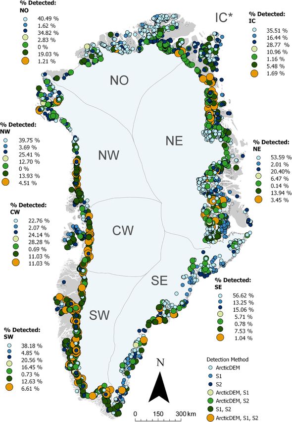
www.nature.com/scientificreports/
small areas using in situ measurements11 and remote sensing25,26, along with forecast modelling to predict future
dynamics13. Remote sensing approaches have also proved advantageous for monitoring water bodies over large
regions of Greenland, such as spectral indices generation from optical and infrared imagery27, classification from
radar imagery28, and sink detection from Digital Elevation Models (DEMs)29. However, each of these remote
sensing approaches has known limitations. For example, ice cover on lakes is understood to limit classification
from optical and SAR imagery28. Therefore, reliance on a single approach can introduce uncertainty through
mis-classification, or underestimation30. An ensemble approach that combines these methods is essential to
successful classification of ice marginal lakes over whole regions with a high degree of certainty31.
This study presents a comprehensive, Greenland-wide inventory of ice marginal lakes for the year 2017 using
a multi-sensor and multi-method approach. Three well-established approaches were used to classify water bodies:
(1) multi-temporal backscatter classification using Sentinel-1 synthetic aperture radar (SAR) imagery (hereafter
referred to as S1); (2) multi-spectral indices classification using Sentinel-2 optical imagery (S2); and (3) sink
detection using the ArcticDEM (ADEM). The results from these approaches were subsequently compiled and
quality-checked to produce the 2017 Inventory of Ice Marginal Lakes (IIML).
Results
Inventory overview. Overall, 4530 polygon features were detected with many overlapping and corre-
sponding to the same ice marginal lake under the combination of the three independent detection methods.
Disregarding multiple counting of overlapping polygons, the IIML indicates that there were 3347 (±8%) unique
ice marginal lakes above a minimum area of 0.05 km 2 (derived as an average of overlapping polygons) in Green-
land in 2017 (Fig. 1). The inventory consists of lakes formed at the ice sheet margin and the margin of Green-
land’s peripheral ice caps and mountain glaciers. This also includes lakes formed around nunataks within 1 km
of the ice sheet margin, based on a modified version of the MEaSUREs GIMP (Greenland Ice Mapping Project)
15 m ice mask (see “Methods” section for more details). A large majority of ice marginal lakes in the inventory
are nameless, with 3194 (95%) unnamed lakes in the IIML based on the Language Secretariat of Greenland
(Oqaasileriffik) placename database.
The highest number of ice marginal lakes are generally present at the longest land-terminating sections of the
GrIS, namely the southwest margin (SW, Fig. 1) and the northeast margin (NE), and the surrounding ice caps
and mountain glaciers (IC). Ice marginal lakes are most abundant around the IC sector, accounting for 28% of
the inventory (948 ice marginal lakes). The SW margin is the most densely populated section of the ice sheet
margin for ice marginal lakes with an average spacing of 5.85 km between each lake (Fig. 2), and includes the
fourth largest of the inventory, Kangaarsuup Tasersua (KT, Fig. 2b).
The least number of ice marginal lakes occur along the central west margin (CW), with only 144 lakes
detected; typically forming in the proglacial area or at the lateral margins of ice sheet outlets such as Eqip Sermia,
Store Glacier (also known as Sermeq Kujalleq) and Lille Glacier (also known as Sermeq Avannarleq) (Fig. S1).
Despite the southeast (SE) being the longest margin at 14,911 km, it is one of the least lake-populated sections
with only 385 ice marginal lakes at an average distancing of 39 km.
Ice marginal lakes are typically smaller than 0.5 km 2, with 2663 lakes (80%) falling within a range between
0.05 and 0.5 km 2 and only 424 lakes larger than 1.00 km 2 (Fig. S2). The largest named ice marginal lake of the
2017 inventory is Romer Sø (130.87 km 2), where the piedmont glacier Elephant Foot Glacier terminates. The
second largest ice marginal lake is Inderhytten (112.02 km 2), a substantial lake at the terminus of Sælsøgletsjer
at the NE margin (Fig. 3). The third largest is an unnamed lake (91.58 km 2 ) along the SW margin, approxi-
mately 100 km south of the settlement of Kangerlussuaq. The largest ice marginal lakes are generally found in
the northern region of the ice sheet margin, with an average area of 1.47 km 2 ( 0.23 km 2 median; 5.76 km 2
standard deviation., Table S1) along the north margin (NO), and an average area of 1.29 km 2 (0.22 km 2 median;
4.00 km 2 standard deviation, Table S1) along the NE margin.
Performance of the methodologies. The majority (74%) of the polygons in the IIML were identified
using only one method, with over half of these instances being ADEM-only (Table S2). Where an ice marginal
lake was detected using two methods (22%), S2 polygons were generally detected along with another method
(making up 723 of 744 of these instances). There are few polygons detected from both ADEM and S1 (21 lakes),
which is likely to reflect the larger number of S2- and ADEM-derived ice marginal lakes in the IIML. Only 199
ice marginal lakes (4%) were detected using all three methods. Successful identification with all three methods
appears to have no visible correlation with lake form or size, but varies according to each section of the GrIS
margin, with the most effective detection occurring along the SW and CW margins (Fig. 4).
From examining the outlines where ice marginal lakes were detected successfully with all three methods,
S1- and S2-derived lakes unsurprisingly had the smallest difference in extent given that these methods detect
water presence directly, with an average areal difference of 0.14 km 2 (Table S3). Larger areal differences are
evident when comparing the ADEM-derived lakes to the S1- and S2-derived lakes, with an average difference of
0.36 km 2 (64%) and 0.25 km 2 (49%), respectively. Taking the maximum and minimum detected extents for each
lake, this produces an average area difference of 0.37 km 2, equating to an areal range of 70% for each lake. This
suggests that the number of methods that successfully identified an ice marginal lake can be used as a measure
of certainty, where ice marginal lakes detected from all three methods (ADEM, S1, S2) denote the highest level
of certainty in lake presence. However, this does not necessarily reflect the lake outline accuracy, given that the
outlines are derived from different time steps.
Scientific Reports | (2021) 11:4481 | https://doi.org/10.1038/s41598-021-83509-1 2
Vol:.(1234567890)
www.nature.com/scientificreports/
Figure 1. Overview of the 2017 ice marginal lake inventory of Greenland, where each defined point represents
one unique ice marginal lake. Ice sheet basins are based on those classified as ice catchments by Mouginot and
Rignot32, with blue points denoting lakes sharing a margin with the ice sheet. Ice marginal lakes adjacent to
Greenland’s ice caps and mountain glaciers are those points in orange, corresponding to the sector statistics
(IC). Figure generated with ArcGIS Pro (v2.6.1, https://www.esri.com/en-us/arcgis/products/arcgis-pro/)66.
Discussion
Multi‑sensor detection methods are needed to encompass latitudinal range of Green‑
land. Successful identification of ice marginal lakes using all three methods used in this study varies accord-
ing to region, with most effective detection occurring at the SW and CW margins (Fig. 4). Of the 681 ice mar-
ginal lakes identified at the SW margin, 248 were detected through two or more sources (36%); as were 73 of the
144 lakes at the CW margin (i.e. 51%) (Table S1). This could be indicative of optimum conditions for detecting
ice marginal lakes (e.g. lack of ice cover) in these regions compared to others.
Other regions are largely composed of lakes detected with just a single source, such as the high abundance
of ADEM-only detected lakes at the NO margin (100 lakes, 40%) and the NE margin (373 lakes, 54%) (Fig. 4,
Table S1). A strength of the ADEM method compared to the S1 and S2 methods is detecting lake basins where
the lake is either partially or completely covered with ice29. This is particularly important in the high-latitude
regions or lakes within a topography with a northern aspect, where ice cover is known to persist throughout the
melt season. Such areas are understood to be notoriously challenging for lake classification from optical and SAR
imagery due to persistent ice cover, even during the summer season10,34. The IIML results reflect this, with the
difference in successful lake classification across each region indicative of the large latitudinal range of climatic
conditions along Greenland. The inclusion of the ADEM method in this study is therefore crucially important,
with ADEM-derived lakes making up nearly half of all the lakes detected across the northern region. These high
latitude lakes would otherwise be unaccounted for in optical and/or SAR-derived lake classifications, and would
result in a marked under-representation of ice marginal lakes in Greenland.
Scientific Reports | (2021) 11:4481 | https://doi.org/10.1038/s41598-021-83509-1 3
Vol.:(0123456789)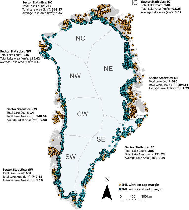
www.nature.com/scientificreports/
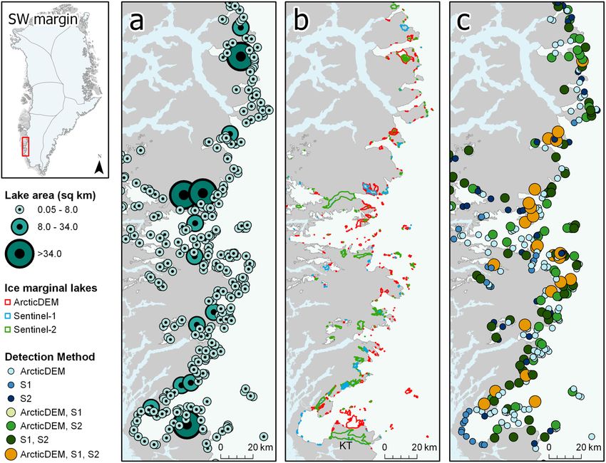
Figure 2. Ice marginal lakes over a selected section of the SW ice sheet margin, where (a) lake area, (b) lake
shape determined by each method (as described in the “Methods” section), and (c) detection method are
presented. Ice, land and ocean are displayed in white, grey and light blue, respectively. The ice margin shown is a
modified version of the MEaSUREs GIMP ice mask33. The largest lake of this region (Kangaarssuup Tasersua) is
labelled as KT in b. Figure generated with ArcGIS Pro (v2.6.1, https://www.esri.com/en-us/arcgis/products/arcgi
s-pro/)66.
Increasing ice marginal lake abundance in West Greenland. The 2017 IIML represents ice mar-
ginal lakes for a discrete time period. The dynamical change of these ice marginal lakes can be better explored
when compared to pre-existing datasets, such as those derived from optical Landsat 4–8 imagery by Carrivick
and Quincey22 for selected years between 1985 and 2011 (1985–1987, 1992–1994, 1999–2001, 2004–2007, and
2009–2011) over the SW and CW margin of the GrIS (excluding IC) (Fig. 5a). A subset of the IIML covering the
same study region is presented for the purpose of this comparison, weighted to the S1- and S2-derived lakes (as
they are detection methods based on the principle of lake inference from water presence, as adopted by Carrivick
and Quincey22). This subset generally reflects the method breakdown of the entire IIML, with 60% of lakes clas-
sified using one method and 40% derived from two or three methods.
A total of 387 (±6.5%) ice marginal lakes were identified along the west margin in the 1985–1988 inventory,
whilst 678 (±8%) lakes have been identified in the 2017 IIML; suggesting a ∼ 75% increase in the number of
lakes along the west margin over the past three decades (Fig. 5b). Minimal changes in total lake area are evident
along the west margin. However, there is a decreasing trend in individual lake area, with average area decreas-
ing from 1.82km 2 (1985–1988) to 0.95km 2 (2017) and median area decreasing from 0.22km 2 (1985–1988) to
0.16km 2 (2017). This trend reflects marked variations in the abundance of small lakes (i.e. 0.05–0.15km 2), and
is suggested to be a possible explanation for the trend in total lake area (Fig. S3). The spatial resolution of these
datasets differ—Carrivick and Q uincey22 primarily used 30 m Landsat imagery whereas the IIML uses data with
a spatial resolution ranging from 5 to 10 m. However, the trend in lake abundance evident in this comparison
is unlikely to be directly attributed to a difference in spatial resolution, given that the minimum lake area is
0.05km 2 in both these records. This comparison therefore suggests an increase in lake abundance across the
west margin of the GrIS.
Scientific Reports | (2021) 11:4481 | https://doi.org/10.1038/s41598-021-83509-1 4
Vol:.(1234567890)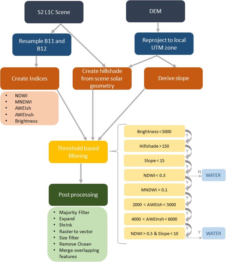
www.nature.com/scientificreports/
Figure 3. Ice marginal lakes over a selected section of the NE ice sheet margin, where (a) lake area, (b)
lake shape determined by each method (as described in the “Methods” section), and (c) detection method
are presented, including the second largest lake of the IIML, Inderhytten (black box). Ice, land and ocean
are displayed in white, grey and light blue, respectively. The ice margin shown is a modified version of the
MEaSUREs GIMP ice mask33. Figure generated with ArcGIS Pro (v2.6.1, https://www.esri.com/en-us/arcgis/
products/arcgis-pro/)66.
Carrivick and Q uincey22 proposed that the changes between 1987 and 2010 were inherently linked to the
0.8% year-1 mean percentage change in ice sheet surface melt35. The results from the 2017 IIML suggest that
increasing lake abundance likely reflects the enhanced retreat of the ice margin, with formation occurring in
front of retreating outlets. Future lake formation is likely to be concentrated in regions where marine-terminating
outlets retreat on to land, as the terrestrial margin length will increase and hold a sinuous form36. Ice marginal
lakes will therefore form a crucial component in the dynamics of these outlets during this transitional p hase37,38.
Additionally, the dynamics of Greenland’s terrestrial store of freshwater will alter if this trend of increasing lake
abundance with decreasing size continues into the future. This could possibly influence the transfer of freshwater
from the GrIS to the ocean, not only affecting melt contribution to the sea level budget, but also with likely effects
on Greenland’s freshwater resources, ecosystems and biogeochemical fl uxes39,40.
High sensitivity in records of remotely‑sensed ice marginal lake change. The multi-method
approach to this study has shown how the choice of method strongly impacts the number of lakes detected; for
instance, 49% of the IIML is derived using the S2 optical method alone. Recent studies into glacial lake change
have relied solely on optical classification approaches, such as the global inventory of glacial lakes presented
by Shugar et al.10 The glacial lake inventory presented by Shugar et al.10 (including ice caps and ice sheets, and
consisting of ice marginal, recently detached proglacial, and near-terminus supraglacial lakes) implemented a
NDWI and NDSI (Normalised Difference Snow Index) approach to classify lakes within a 1 km buffer of the ice
margin. The glacial lake inventory suggested an overall increase of 53% in the number of lakes between 1990–
1999 (9414 lakes) and 2015–2018 (14,393 lakes), with a total area growth of 51%. Of those glacial lakes detected
in Greenland in 2015–2018, only 44% corresponded with ice marginal lakes from the current study (the IIML),
suggesting that up to 56% of ice marginal lakes in Greenland remain unaccounted for in current global estimates.
Scientific Reports | (2021) 11:4481 | https://doi.org/10.1038/s41598-021-83509-1 5
Vol.:(0123456789)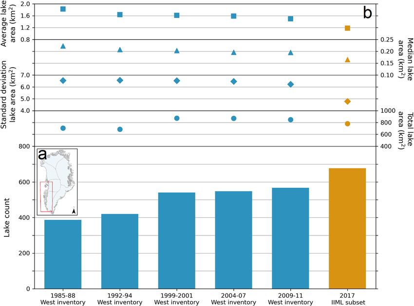
www.nature.com/scientificreports/
Figure 4. The number of detection methods that successfully classified each ice marginal lake, split by region
with percentage breakdowns of each combination of detection methods (see Table S1 for further details). Ice
sheet basins are based on those classified as ice catchments by Mouginot and R ignot32. Figure generated with
ArcGIS Pro (v2.6.1, https://www.esri.com/en-us/arcgis/products/arcgis-pro/)66. *IC denotes ice marginal lakes
found at the margins of Greenland’s ice caps and mountain glaciers.
Whilst this could be a result of the differing resolutions of the IIML (10 m spatial resolution for 2017) and the
glacial lake inventory from Shugar et al.10 (30 m spatial resolution for 2015–2018), it is also likely that the wider
range of classification approaches used in the IIML results in better lake identification under varying environ-
mental and imaging conditions, such as the challenges with cloud cover in optical satellite scenes, ice-covered
lakes, and lake water turbidity. This highlights a trade-off between classification accuracy and study feasibility,
where multi-method implementations for producing global datasets demand more time and processing power
at the expense of reduced accuracy.
Scientific Reports | (2021) 11:4481 | https://doi.org/10.1038/s41598-021-83509-1 6
Vol:.(1234567890)www.nature.com/scientificreports/
Figure 5. Change in ice marginal lakes along the west margin of the GrIS, where (a) shows the west margin
sector and (b) the ice marginal lake time-series from 1985 to 2017. The square point plot (top) denotes average
lake area, the circle point plot (middle) shows total lake area, and the bar plot (bottom) depicts lake count. All
inventories between 1985–1988 and 2009–2011 (blue) are as presented by Carrivick and Q uincey22. Data points
from 2017 are a subset taken from the IIML presented in this study (orange). The subset covers the same sector
of the west margin, where the S1- and S2-derived lakes are preferenced as alike methods to the Landsat-derived
lakes, based on the principle of lake inference from water presence. The 2017 values presented are an average of
the subset with and without ADEM-only lakes, thereby preferencing S1- and S2-derived lakes, but still including
lakes identified using the ADEM method.
Greenland-wide estimates of ice marginal lake extent are highly sensitive to mis-classifications. For example,
Inderhytten is the second largest ice marginal lake in Greenland (as shown in Fig. 3) at 112.02km 2 according to
the IIML. However, Inderhytten is not included in the glacial lake inventory presented by Shugar et al.10 because
it is ice covered for the majority of the year and lies at an elevation below the threshold of their classification (< 5
m a.s.l.). The absence of Inderhytten would modify the dataset substantially if left out of the IIML, skewing the
average lake size and total area of the dataset by 4%. Such a substantial impact on Greenland-wide estimates not
only draws attention to the problem of mis-classifications, but also demonstrates the potential of implementing
multi-sensor and multi-method approaches in lake detection to reliably and accurately define ice marginal lake
change.
Conclusions
The Greenland-wide inventory of ice marginal lakes uncovers 3347 (±8%) unique lakes (above 0.05km 2) in 2017,
using a multi-method approach incorporating backscatter classification from Sentinel-1 satellite imagery, multi-
spectral indices classification from Sentinel-2 satellite imagery, and sink detection from the high-resolution Arc-
ticDEM. The average lake size of the entire inventory is 0.88km 2 with the largest being Romer Sø (130.87km 2),
situated on the NE margin of the GrIS. A high number of lakes are around Greenland’s ice caps and mountain
glaciers, and along the SW margin of the ice sheet, collectively accounting for nearly half (49%) of the inventory.
The multi-method approach provides an effective means of evaluating the certainty of each detected ice
marginal lake. Overall, 26% of the inventory was identified with two or more methods, with a high majority of
those identified using the sink detection method. Successful identification with all three methods has no correla-
tion with lake form or size, but does appear to be region-dependent with the most effective detection occurring
along the SW and CW margins. This likely reflects the optimum climatic conditions in these regions, such as
the lack of summer ice cover.
Greenland-wide estimates of ice marginal lake change are impeded by method limitations in remote sensing,
which can lead to mis-classifications and under-representation of lakes. Comparison to a recent global glacial
Scientific Reports | (2021) 11:4481 | https://doi.org/10.1038/s41598-021-83509-1 7
Vol.:(0123456789)www.nature.com/scientificreports/
lakes inventory suggests that over half of ice marginal lake changes could be unaccounted for in current global
estimates, with only 44% of lakes from the IIML (presented in this study) accounted for in a global glacial lake
inventory10. The lake detection and filtering methods have to be carefully selected and might not be applicable
to all regions in the same combination. For Greenland, only the multi-sensor and multi-method approaches
applied here provided satisfactory results and a solid baseline dataset for change assessment. This highlights the
power and potential that the increasing availability of high-resolution global satellite remote sensing datasets
from different sensors (optical, radar, stereo etc.) and the improving computational possibilities to process and
analyse such big amounts of data offers for environmental mapping and monitoring in general.
Lake change analysis along the west margin of the GrIS suggests a ∼ 75% increase in the number of ice
marginal lakes over the past three decades since 1 98522. This trend likely follows increases in melt runoff and
the retreating ice margin, with new lake formation occurring in front of retreating outlets. This suggests that ice
marginal lakes will be of growing importance to the terrestrial store of water in Greenland. Glacier dynamics
and mass balance are also influenced by lake termination, hence lake evolution can have significant effects on ice
flow and melt and is not just a passive result of changes in ice margin position. Not only will ice marginal lakes
likely be a significant dynamic component in future sea level contribution from the GrIS, but they will also have
implications for freshwater resource management and ecosystems in Greenland which need to be examined in
long-term monitoring strategies. Overall, this inventory provides a benchmark to conduct further analysis from,
and develop our understanding of ice marginal lake dynamics on a Greenland-wide scale.
Methods
Sentinel‑1 multi‑temporal backscatter classification. Open permanent water bodies were identified
from Sentinel-1 SAR images acquired during 2017. Over Greenland, Sentinel-1 was operated in the Interfero-
metric Wide Swath (IWS) mode at Horizontal–Horizontal (HH) and Horizontal–Vertical (HV) polarisation
with a repeat-pass of 12 days. The SAR images were provided by the European Space Agency (ESA) in Ground
Range Detected (GRD) format with a pixel size of 10 m. Each image was averaged to the original spatial resolu-
tion of the data (20 m) and calibrated to gamma0 using an ArcticDEM m osaic41. Each image was then trans-
formed from the radar acquisition geometry to the map geometry using a geocoding look-up table, created
using the orbital information, SAR image processing parameters, and the ArcticDEM mosaic42,43. The geocoded
images were finally tiled to a predefined grid of 100 × 100 km large blocks for easier data handling. From the
individual images of the SAR backscattered intensity, monthly averages per polarisation (AVE) were derived to
overcome the issue of speckle noise in a single image:
N
1
AVE = 10 ∗ log Ii (1)
N
i=1
where Ii is the SAR backscatter, and i is between 1 and N (i.e. the number of SAR observations at a given pixel
in a given month, for a given polarisation).
Water bodies were detected using an ensemble-bagged tree classifier applied to the set of 24 predictors
consisting of the 12 monthly SAR backscatter average values for each polarization. Including the entire time
series of observations in the classifier served to reduce water commission errors introduced by wet snow and ice
conditions, in which case the SAR backscatter is similar to the level observed over open w ater44. The classifier
was trained with samples extracted from a water classification of SPOT images covering the Disko Bay. Lacking
a similar dataset for the rest of Greenland, it was assumed that the classification rules based on the Disko Bay
area would be equally applicable throughout the country.
Classification errors were limited through a set of post-processing steps which included the removal of iso-
lated pixels and polygons smaller than 15 pixels, and removal of water bodies located on slopes steeper than 10◦
according to the ArcticDEM mosaic44,45. This 15-pixel threshold was determined from testing with increasing
thresholds, where 15 pixels turned out to be the optimum value for adequate removal of false detection whilst
preserving small positive classifications.
Sentinel‑2 multi‑spectral indices classification. Standard TOA (Top-Of-Atmosphere) Sentinel-2 L1C
scenes were used in this study because standard surface reflectance products were not available at the time of
processing. The standard TOA scenes were used as atmospheric corrections over Greenland are complex and
have a risk of introducing sources of e rror46. Scenes were automatically selected based on cloud cover (< 50%)
over July and August 2017 in order to limit lake ice and snow cover and maximise successful water classification.
These Sentinel-2 scenes were processed in the local UTM projection (UTM Zone 24N), and bands 11 and 12
were re-sampled from 20 to 10 m using a nearest neighbour approach.
Water bodies were classified using a multi-terrain and multi-spectral indices approach through the processing
chain as demonstrated in Fig. 631,47. The multi-terrain indices consists of a slope and aspect index calculated from
sun geometry (available in the scene metadata) in relation to topography slope and a spect48. The multi-terrain
indices distinguishes regions at risk to false positive detection caused by topographic shadowing and sun glint,
and are subsequently masked out31,49.
The multi-spectral indices are a collection of well-established spectral indices—NDWI, MNDWI, AWEIsh,
AWEInsh and brightness (Table 1)—which are passed through a multi-layer decision tree classification to clas-
sify water bodies (Fig. 6). A coarse brightness threshold (more typically referred to as grayscale transformation)
is applied, which acts as a simple initial filter for removing regions where highly reflective snow and ice are
present. The NDWI and MNDWI are highly effective at detecting optically clear water bodies not affected by
shadowing47,49–51. The AWEIsh and AWEInsh indices are effective at detecting and preserving water bodies with
Scientific Reports | (2021) 11:4481 | https://doi.org/10.1038/s41598-021-83509-1 8
Vol:.(1234567890)www.nature.com/scientificreports/
Figure 6. Flow diagram presenting the processing chain for classifying ice marginal lakes from Sentinel-2
imagery, including terrain indices generation using a DEM and multi-spectral indices thresholding, which is
compiled through a decision tree classifier to extract water bodies.
Index Expression (Sentinel-2 bands) Strengths and target References
NDWI (normalised difference water index) ( B3 − B8)/(B3 + B8) Water and shadow, sediment-loaded water and snow/ice McFeeters53
MNDWI (modified normalised difference water index) (B3 − B11)/(B3 + B11) Water and snow and ice Xu54
AWEIsh (automatic water extraction index shadow) B2 + 2.5 ∗ B3 − 1.5 ∗ (B8 + B11) − 0.25 ∗ B12 Sediment-loaded water Feyisa et al.52
AWEInsh (automatic water extraction index no shadow) 4 ∗ (B3 − B11) − (0.25 ∗ B8 + 2.75 ∗ B12) Sediment-loaded water Feyisa et al.52
Brightness (B4 + B3 + B2)/3 Snow covered areas –
Table 1. Description of each of the spectral indices used in this study and their detection strengths.
higher sediment loads, such as those with a high percentage of glacial rock fl our52. In combination, the multi-
spectral indices are an effective approach to successful water classification by utilising the strength of each index.
After applying a threshold-based filtering to each of the indices, a series of post-processing stages were applied.
These post-processing stages included raster-to-polygon conversion of the classified water bodies, applying an
ocean mask, merging the overlapping polygon features, and applying a minimum area threshold of 0.05km 2 to
the merged polygons.
Scientific Reports | (2021) 11:4481 | https://doi.org/10.1038/s41598-021-83509-1 9
Vol.:(0123456789)www.nature.com/scientificreports/
ArcticDEM sink detection. Basins were classified from the ArcticDEM 10 m mosaic (Release 7, Version
3.0, https://www.pgc.umn.edu/data/arcticdem/) using a sink detection approach, commonly used for extracting
large-scale topographic structures such as watersheds, streams and depressions55. The ArcticDEM is derived
from high-resolution commercial optical stereo satellite imagery, generated through an adapted version of the
automated Ames Stereo Pipeline56,57. The ArcticDEM mosaic is comprised of strip data acquired between 2009
and 2017, which is averaged, filtered and validated against filtered IceSAT altimetry data. Whilst the ArcticDEM
mosaic does not represent a discrete time step, it was included in this study over the raw strip data because of the
known limitations with using the strip data, namely limited accuracy, heavy reliance on validation datasets, and
inhibited study f easibility58,59. Therefore, basins detected from the ArcticDEM mosaic reflect a temporal average
and are not indicative of conditions at a specific time.
Sinks were defined by filling topographic depressions in the DEM to its pour point (i.e. the minimum eleva-
tion along its watershed boundary), following which the original DEM elevation value was subtracted from the
depression-filled DEM elevation value60. Shallow sinks (< 5 m deep, or < 0.05 km 2 areal extent) were filtered to
remove mis-classifications and water bodies with an insignificant water drainage volume, and limit the risk of
discounting sinks that are consistently at, or exceeding, their pour p oint25.
Dataset compiling. The water bodies derived from each approach (S1, S2 and ADEM) were combined and
filtered in a semi-automated fashion. Water bodies were masked using a 1 km buffer around a modified version
of the MEaSUREs GIMP 15 m ice mask (produced from a 1999 to 2001 image mosaic, https://nsidc.org/data/
NSIDC-0714/versions/1)33,61. The ice mask was modified manually using coinciding Sentinel-2 imagery and a
Landsat 8 image m osaic62 to update marked changes in the ice margin and outlet positions. Finally, the inven-
tory was filtered and verified manually for quality purposes, as is standard practise in similar studies such as
those looking at the H imalaya63–65. Detected features were removed from the inventory if they were not water
filled or did not have any visible sign of drainage (such as waterline marks), based on manual validation against
coinciding Sentinel-2 optical imagery. Following this, the dataset was populated with the appropriate metadata
including detection method/s, basin location (based on those defined by Mouginot and Rignot32, https://nsidc
.org/data/NSIDC-0714/versions/1), and lake name (provided by the Language Secretariat of Greenland, Oqaa-
sileriffik, placename database).
Error estimation. Error analysis was conducted to estimate the certainty of lake presence in the IIML (i.e.
lake frequency). Four discrete 10,000km 2 regions were selected to conduct the error analysis, covering the NE,
NW and SW margins, and including the IC sector. Two independent users manually defined ice marginal lakes
in each of these regions, using cloud-free Sentinel-2 imagery captured within the acquisition period that the
IIML was derived (01/08-13/09/2017). The users defined an ice marginal lake using a single annotated point
overlapping with the location of the lake on the Sentinel-2 image. The user-defined ice marginal lakes were com-
pared to those from the IIML to determine differences in the number of lakes present in each region. A success-
ful match is deemed as a user-defined point that is either overlapping or within 10 m of a polygon from the IIML.
Each region in the error analysis had an average of 68 lakes present, with a maximum number of 100 lakes, as
defined by the two users. There was minimal discrepancy between the users, with an average difference of three
lakes per 10,000km 2 region. User-defined lakes below a surface area of 0.05km 2 were then removed to match the
size threshold of the IIML. Overlap analysis was performed to determine corresponding lakes between the user-
defined datasets and the IIML. Overall, the IIML captured 92% of the user-defined ice marginal lakes. This forms
an error estimate for lake frequency in the IIML of ±8%, or ±201 lakes, as reported in the presented results.
Data availability
The 2017 inventory of ice marginal lakes is a data product under the ESA Glaciers CCI (Climate Change Initia-
tive), freely available through the CEDA (Centre for Environmental Data Analysis) Archive at https://catalogue.
ceda.ac.uk/uuid/7ea7540135f441369716ef867d217519.
Received: 16 October 2020; Accepted: 2 February 2021
References
1. IPCC. IPCC Special Report on the Ocean and Cryosphere in a Changing Climate (2019).
2. Mouginot, J. et al. Forty-six years of Greenland Ice Sheet mass balance from 1972 to 2018. PNAS 116, 9239–9244. https://doi.
org/10.1073/pnas.1904242116 (2019).
3. Hanna, E. Greenland surface air temperature changes from 1981 to 2019 and implications for ice-sheet melt and mass-balance
change. Int. J. Climatol. 41, E1336–E1352. https://doi.org/10.1002/joc.6771 (2021).
4. Shepherd, A. et al. Mass balance of the Greenland Ice Sheet from 1992 to 2018. Nature 579, 233–239. https: //doi.org/10.1038/s4158
6-019-1855-2 (2020).
5. Lewis, S. M. & Smith, L. C. Hydrologic drainage of the Greenland Ice Sheet. Hydrol. Process. 23, 2004–2011. https: //doi.org/10.1002/
hyp.7343 (2009).
6. Haeberli, W. & Linsbauer, A. Brief communication “Global glacier volumes and sea level—Small but systematic effects of ice below
the surface of the ocean and of new local lakes on land’’. Cryosphere 7, 817–821. https://doi.org/10.5194/tc-7-817-2013 (2013).
7. Loriaux, T. & Casassa, G. Evolution of glacial lakes from the Northern Patagonia Icefield and terrestrial water storage in a sea-level
rise context. Glob. Planet Change 102, 33–40. https://doi.org/10.1016/j.gloplacha.2012.12.012 (2013).
8. Huss, M. & Hock, R. A new model for global glacier change and sea-level rise. Front. Earth Sci. 3, 54. https://doi.org/10.3389/feart
.2015.00054(2015).
9. Sutherland, J. L. et al. Proglacial lakes control glacier geometry and behavior during recession. Geophys. Res. Lett. 47,
e2020GL088865. https://doi.org/10.1029/2020GL088865 (2020).
Scientific Reports | (2021) 11:4481 | https://doi.org/10.1038/s41598-021-83509-1 10
Vol:.(1234567890)www.nature.com/scientificreports/
10. Shugar, D. H. et al. Rapid worldwide growth of glacial lakes since 1990. Nat. Clim. Change. 10, 939–945. https://doi.org/10.1038/
s41558-020-0855-4 (2020).
11. Russell, A. J., Carrivick, J. L., Ingeman-Nielsen, T., Yde, J. C. & Williams, M. A new cycle of jökulhlaups at Russell Glacier, Kanger-
lussuaq, West Greenland. J. Glaciol. 57, 238–246. https://doi.org/10.3189/002214311796405997 (2011).
12. Wolfe, D.F.G., Kargel, J.S. & Leonard, G.J. Glacier-dammed ice-marginal lakes of Alaska. in Kargel, J.S., Leonard, G.J., Bishop, M.P.,
Kääb, A. & Raup, B.H. (eds.) Global Land Ice Measurements from Space, Springer Praxis Books 263–295 (Springer, Berlin, 2014).
13. Carrivick, J. L. et al. Ice-dammed lake drainage evolution at Russell Glacier, West Greenland. Front. Earth Sci. 5, 100. https://doi.
org/10.3389/feart.2017.00100 (2017).
14. Carrivick, J. L. & Tweed, F. S. A review of glacier outburst floods in Iceland and Greenland with a megafloods perspective. Earth.
Sci. Rev. 196, 102876. https://doi.org/10.1016/j.earscirev.2019.102876 (2019).
15. Anderson, N. J. et al. The arctic in the twenty-first century: Changing biogeochemical linkages across a paraglacial landscape of
greenland. BioScience 67, 118–133. https://doi.org/10.1093/biosci/biw158 (2017).
16. Storms, J. E. A., de Winter, I. L., Overeem, I., Drijkoningen, G. G. & Lykke-Andersen, H. The Holocene sedimentary history of the
Kangerlussuaq Fjord-valley fill, West Greenland. Quat. Sci. Rev. 35, 29–50. https://doi.org/10.1016/j.quascirev.2011.12.014 (2012).
17. Kjeldsen, K. K. et al. Ice-dammed lake drainage cools and raises surface salinities in a tidewater outlet glacier fjord, west Greenland.
J. Geophys. Res. Earth Surf. 119, 1310–1321. https://doi.org/10.1002/2013JF003034 (2014).
18. Higgins, A. K. On some ice-dammed lakes in Frederikshåb district, south-West Greenland. Medd. Dansk Geol. Foren. 19, 378–397
(1970).
19. Weidick, A. & Citterio, M. The ice-dammed lake Isvand, West Greenland, has lost its water. J. Glaciol. 57, 186–188. https://doi.
org/10.3189/002214311795306600 (2011).
20. Carrivick, J. L., Turner, A. G. D., Russell, A. J., Ingeman-Nielsen, T. & Yde, J. C. Outburst flood evolution at Russell Glacier, western
Greenland: Effects of a bedrock channel cascade with intermediary lakes. Quat. Sci. Rev. 67, 39–58. https: //doi.org/10.1016/j.quasc
irev.2013.01.023 (2013).
21. McGrath, D. et al. Sediment plumes as a proxy for local ice-sheet runoff in Kangerlussuaq Fjord, West Greenland. J. Glaciol. 56,
813–821. https://doi.org/10.3189/002214310794457227 (2010).
22. Carrivick, J. L. & Quincey, D. J. Progressive increase in number and volume of ice-marginal lakes on the western margin of the
Greenland Ice Sheet. Glob. Planet. Change 116, 156–163. https://doi.org/10.1016/j.gloplacha.2014.02.009 (2014).
23. Mernild, S. H. & Hasholt, B. Observed runoff, jökulhlaups and suspended sediment load from the Greenland ice sheet at Kanger-
lussuaq, West Greenland, 2007 and 2008. J. Glaciol. 55, 855–858. https://doi.org/10.3189/002214309790152465 (2009).
24. Harrison, S. et al. Climate change and the global pattern of moraine-dammed glacial lake outburst floods. Cryosphere 12, 1195–
1209. https://doi.org/10.5194/tc-12-1195-2018 (2018).
25. Larsen, M. A. D. et al. A satellite perspective on jökulhlaups in Greenland. Hydrol. Res. 44, 68–77. https://doi.org/10.2166/
NH.2012.195 (2013).
26. Mallalieu, J., Carrivick, J. L., Quincey, D. J. & Smith, M. W. Calving seasonality associated with melt-undercutting and lake ice
cover. Geophys. Res. Lett. 47, e2019GL086561. https://doi.org/10.1029/2019GL086561 (2020).
27. Williamson, A. G., Arnold, N. S., Banwell, A. F. & Willis, I. C. A Fully automated Supraglacial lake area and volume Tracking
(“FAST”) algorithm: Development and application using MODIS imagery of West Greenland. Remote Sens. Environ. 196, 113–133.
https://doi.org/10.1016/j.rse.2017.04.032 (2017).
28. Miles, K. E., Willis, I. C., Benedek, C. L., Williamson, A. G. & Tedesco, M. Toward monitoring surface and subsurface lakes on
the greenland ice sheet using sentinel-1 SAR and landsat-8 OLI imagery. Front. Earth Sci. 5, 58. https://doi.org/10.3389/feart
.2017.00058(2017).
29. Pope, A. et al. Estimating supraglacial lake depth in West Greenland using Landsat 8 and comparison with other multispectral
methods. Cryosphere 10, 15–27. https://doi.org/10.5194/tc-10-15-2016 (2016).
30. Leeson, A. A. et al. A comparison of supraglacial lake observations derived from MODIS imagery at the western margin of the
Greenland ice sheet. J. Glaciol. 59, 1179–1188. https://doi.org/10.3189/2013JoG13J064 (2013).
31. Wangchuk, S. & Bolch, T. Mapping of glacial lakes using Sentinel-1 and Sentinel-2 data and a random forest classifier: Strengths
and challenges. Sci. Remote Sens. 2, 100008. https://doi.org/10.1016/j.srs.2020.100008 (2020).
32. Mouginot, J. & Rignot, E. Glacier catchments/basins for the Greenland Ice Sheet. UC Irvine Dataset.https: //doi.org/10.7280/D1WT1
1 (2019).
33. Howat, I. MEaSUREs Greenland Ice Mapping Project (GIMP) land ice and ocean classification mask, version 1 [GimpIceMask
15 m tiles 0-5]. NASA National Snow and Ice Data Center Distributed Active Archive Center, Boulder, Colorado USA. https://doi.
org/10.5067/B8X58MQBFUPA (2017).
34. Strozzi, T., Wiesmann, A., Kääb, A., Joshi, S. & Mool, P. Glacial lake mapping with very high resolution satellite SAR data. Nat.
Hazards Earth Syst. Sci. 12, 2487–2498. https://doi.org/10.5194/nhess-12-2487-2012 (2012).
35. Hanna, E. et al. Increased runoff from melt from the greenland ice sheet: A response to global warming. J. Clim. 21, 331–341. https
://doi.org/10.1175/2007JCLI1964.1 (2008).
36. Mernild, S. H., Malmros, J. K., Yde, J. C. & Knudsen, N. T. Multi-decadal marine- and land-terminating glacier recession in the
Ammassalik region, southeast Greenland. Cryosphere 6, 625–639. https://doi.org/10.5194/tc-6-625-2012 (2012).
37. Carrivick, J. L., Tweed, F. S., Sutherland, J. L. & Mallalieu, J. Toward numerical modeling of interactions between ice-marginal
proglacial lakes and glaciers. Front. Earth Sci. 8, 577068. https://doi.org/10.3389/feart.2020.577068 (2020).
38. Catania, G.A., Stearns, L.A., Moon, T.A., Enderlin, E.M. & Jackson, R.H. Future evolution of Greenland’s marine-terminating
outlet glaciers. J. Geophys. Res. Earth Surface 125, e2018JF004873. https://doi.org/10.1029/2018JF004873 (2020).
39. Christensen, T. R., Arndal, M. F. & Topp-Jørgensen, E. Greenland Ecosystem Monitoring Annual Report Cards 2019 (Aarhus Uni-
versity, DCE—Danish Centre for Environment and Energy, 2020).
40. Hopwood, M. J. et al. Review article: How does glacier discharge affect marine biogeochemistry and primary production in the
Arctic? Cryosphere 14, 1347–1383. https://doi.org/10.5194/tc-14-1347-2020 (2020).
41. Frey, O., Santoro, M., Werner, C. L. & Wegmuller, U. DEM-based SAR pixel-area estimation for enhanced geocoding refinement
and radiometric normalization. IEEE Geosci. Remote Sens. Lett. 10, 48–52. https://doi.org/10.1109/LGRS.2012.2192093 (2013).
42. Wegmüller, U. Automated terrain corrected SAR geocoding. Proc. IGARSS’99 3, 1712–1714. https://doi.org/10.1109/IGARS
S.1999.772070 (1999). (IEEE, Hamburg, Germany).
43. Wegmüller, U., Werner, C., Strozzi, T. & Wiesmann, A. Automated and precise image registration procedures. in Analysis of Multi-
Temporal Remote Sensing Images, Series in Remote Sensing, vol. 2, 37–49 (World Scientific, 2002).
44. Santoro, M. & Wegmüller, U. Multi-temporal synthetic aperture radar metrics applied to map open water bodies. IEEE J. Sel. Top.
Appl. Earth Obs. Remote Sens. 7, 3225–3238. https://doi.org/10.1109/JSTARS.2013.2289301 (2014).
45. Santoro, M. et al. Strengths and weaknesses of multi-year Envisat ASAR backscatter measurements to map permanent open water
bodies at global scale. Remote Sens. Environ. 171, 185–201. https://doi.org/10.1016/j.rse.2015.10.031 (2015).
46. Williamson, A. G., Banwell, A. F., Willis, I. C. & Arnold, N. S. Dual-satellite (Sentinel-2 and Landsat 8) remote sensing of suprag-
lacial lakes in Greenland. Cryosphere 12, 3045–3065. https://doi.org/10.5194/tc-12-3045-2018 (2018).
47. Chen, F., Zhang, M., Tian, B. & Li, Z. Extraction of glacial lake outlines in Tibet Plateau using landsat 8 imagery and google earth
engine. IEEE J. Sel. Top. Appl. Earth Obs. Remote Sens. 10, 4002–4009. https://doi.org/10.1109/JSTARS.2017.2705718 (2017).
Scientific Reports | (2021) 11:4481 | https://doi.org/10.1038/s41598-021-83509-1 11
Vol.:(0123456789)www.nature.com/scientificreports/
48. Burrough, P. A., McDonnell, R., McDonnell, R. A. & Lloyd, C. D. Principles of Geographical Information Systems 3rd edn. (Oxford
University Press, Oxford, 2015).
49. Feng, M., Sexton, J. O., Channan, S. & Townshend, J. R. A global, high-resolution (30-m) inland water body dataset for 2000:
First results of a topographic-spectral classification algorithm. Int. J. Digit. Earth 9, 113–133. https://doi.org/10.1080/17538
947.2015.1026420 (2016).
50. Huggel, C., Kääb, A., Haeberli, W., Teysseire, P. & Paul, F. Remote sensing based assessment of hazards from glacier lake outbursts:
A case study in the Swiss Alps. Can. Geotech. J. 39, 316–330. https://doi.org/10.1139/t01-099 (2002).
51. Bolch, T., Buchroithner, M. F., Peters, J., Baessler, M. & Bajracharya, S. Identification of glacier motion and potentially dangerous
glacial lakes in the Mt. Everest region/Nepal using spaceborne imagery. Nat. Hazards Earth Syst. Sci. 8, 1329–1340. https://doi.
org/10.5194/nhess-8-1329-2008 (2008).
52. Feyisa, G. L., Meilby, H., Fensholt, R. & Proud, S. R. Automated Water Extraction Index: A new technique for surface water map-
ping using Landsat imagery. Remote Sens. Environ. 140, 23–35. https://doi.org/10.1016/j.rse.2013.08.029 (2014).
53. McFeeters, S. K. The use of the Normalized Difference Water Index (NDWI) in the delineation of open water features. Int. J. Remote
Sens. 17, 1425–1432. https://doi.org/10.1080/01431169608948714 (1996).
54. Xu, H. Modification of normalised difference water index (NDWI) to enhance open water features in remotely sensed imagery.
Int. J. Remote Sens. 27, 3025–3033. https://doi.org/10.1080/01431160600589179 (2006).
55. Jenson, S. K. & Domingue, J. O. Extracting topographic structure from digital elevation data for geographic information-system
analysis. Photogramm. Eng. Rem. Sens. 54, 1593–1600 (1988).
56. Shean, D. E. et al. An automated, open-source pipeline for mass production of digital elevation models (DEMs) from very-high-
resolution commercial stereo satellite imagery. ISPRS J. Photogramm. Remote Sens. 116, 101–117. https://doi.org/10.1016/j.isprs
jprs.2016.03.012 (2016).
57. Porter, C. et al. ArcticDEM. Hardvard Dataverse.https://doi.org/10.7910/DVN/OHHUKH (2018).
58. Błaszczyk, M. et al. Quality assessment and glaciological applications of digital elevation models derived from space-borne and
aerial images over two tidewater glaciers of Southern Spitsbergen. Remote Sens. 11, 1121. https://doi.org/10.3390/rs11091121
(2019).
59. Bowling, J. S., Livingstone, S. J., Sole, A. J. & Chu, W. Distribution and dynamics of Greenland subglacial lakes. Nat. Commun. 10,
2810. https://doi.org/10.1038/s41467-019-10821-w (2019).
60. Planchon, O. & Darboux, F. A fast, simple and versatile algorithm to fill the depressions of digital elevation models. CATENA 46,
159–176. https://doi.org/10.1016/S0341-8162(01)00164-3 (2002).
61. Howat, I. M., Negrete, A. & Smith, B. E. The Greenland Ice Mapping Project (GIMP) land classification and surface elevation data
sets. Cryosphere 8, 1509–1518. https://doi.org/10.5194/tc-8-1509-2014 (2014).
62. Chen, Z. et al. A new image mosaic of Greenland using Landsat-8 OLI images. Sci. Bull. 65, 522–524. https://doi.org/10.1016/j.
scib.2020.01.014 (2020).
63. Nie, Y., Liu, Q. & Liu, S. Glacial lake expansion in the Central Himalayas by Landsat Images, 1990–2010. PLOS ONE 8, e83973.
https://doi.org/10.1371/journal.pone.0083973 (2013).
64. Aggarwal, S., Rai, S. C., Thakur, P. K. & Emmer, A. Inventory and recently increasing GLOF susceptibility of glacial lakes in Sikkim,
Eastern Himalaya. Geomorphology 295, 39–54. https://doi.org/10.1016/j.geomorph.2017.06.014 (2017).
65. Shukla, A., Garg, P. K. & Srivastava, S. Evolution of glacial and high-altitude lakes in the Sikkim, Eastern Himalaya over the past
four decades (1975–2017). Front. Environ. Sci. 6, 81. https://doi.org/10.3389/fenvs.2018.00081 (2018).
66. Esri Inc. ArcGIS Pro (v2.6.1) (2020).
Acknowledgements
This work is funded by the ESA (4000109873/14/I-NB) Glaciers CCI (Climate Change Initiative) Phase 2, Option
6, titled ‘An Inventory of Ice-Marginal Lakes in Greenland’. We would like to thank Stephen Plummer for his
technical feedback during the course of this work.
Author contributions
P.H. drafted the manuscript and AM produced the manuscript figures. P.H., A.M., E.M., K.L. and M.B. coordi-
nated the optical classification and sink detection workflow, and performed the post-processing, manual cleaning
and compiling of the IIML. M.S., A.W. and R.C. coordinated and performed the SAR classification workflow. F.P.
and A.K. managed the project and its peripheral activities. J.L.C. provided the comparison inventory datasets.
All authors contributed to the preparation of the manuscript.
Competing interests
The authors declare no competing interests.
Additional information
Supplementary Information The online version contains supplementary material available at https://doi.
org/10.1038/s41598-021-83509-1.
Correspondence and requests for materials should be addressed to P.H.
Reprints and permissions information is available at www.nature.com/reprints.
Publisher’s note Springer Nature remains neutral with regard to jurisdictional claims in published maps and
institutional affiliations.
Scientific Reports | (2021) 11:4481 | https://doi.org/10.1038/s41598-021-83509-1 12
Vol:.(1234567890)www.nature.com/scientificreports/
Open Access This article is licensed under a Creative Commons Attribution 4.0 International
License, which permits use, sharing, adaptation, distribution and reproduction in any medium or
format, as long as you give appropriate credit to the original author(s) and the source, provide a link to the
Creative Commons licence, and indicate if changes were made. The images or other third party material in this
article are included in the article’s Creative Commons licence, unless indicated otherwise in a credit line to the
material. If material is not included in the article’s Creative Commons licence and your intended use is not
permitted by statutory regulation or exceeds the permitted use, you will need to obtain permission directly from
the copyright holder. To view a copy of this licence, visit http://creativecommons.org/licenses/by/4.0/.
© The Author(s) 2021
Scientific Reports | (2021) 11:4481 | https://doi.org/10.1038/s41598-021-83509-1 13
Vol.:(0123456789)You can also read