Scaling of instability timescales of Antarctic outlet glaciers based on one-dimensional similitude analysis - The Cryosphere
←
→
Page content transcription
If your browser does not render page correctly, please read the page content below
The Cryosphere, 13, 1621–1633, 2019
https://doi.org/10.5194/tc-13-1621-2019
© Author(s) 2019. This work is distributed under
the Creative Commons Attribution 4.0 License.

Scaling of instability timescales of Antarctic outlet glaciers
based on one-dimensional similitude analysis
Anders Levermann1,2,3 and Johannes Feldmann1
1 Potsdam   Institute for Climate Impact Research (PIK), Potsdam, Germany
2 LDEO,    Columbia University, New York, USA
3 Institute of Physics, University of Potsdam, Potsdam, Germany

Correspondence: Anders Levermann (anders.levermann@pik-potsdam.de)

Received: 15 November 2018 – Discussion started: 15 January 2019
Revised: 12 April 2019 – Accepted: 3 May 2019 – Published: 13 June 2019

Abstract. Recent observations and ice-dynamic modeling             2018). Large parts of the Antarctic Ice Sheet rest on a ret-
suggest that a marine ice-sheet instability (MISI) might           rograde marine bed, i.e., on a bed topography that lies be-
have been triggered in West Antarctica. The correspond-            low the current sea level and is downsloping inland (Bent-
ing outlet glaciers, Pine Island Glacier (PIG) and Thwaites        ley et al., 1960; Ross et al., 2012; Cook and Swift, 2012;
Glacier (TG), showed significant retreat during at least the       Fretwell et al., 2013). This topographic situation makes these
last 2 decades. While other regions in Antarctica have the to-     parts of the ice sheet prone to a so-called marine ice-sheet
pographic predisposition for the same kind of instability, it is   instability (MISI; Weertman, 1974; Mercer, 1978; Schoof,
so far unclear how fast these instabilities would unfold if they   2007; Pattyn, 2018). Currently, this kind of instability con-
were initiated. Here we employ the concept of similitude to        stitutes a large uncertainty in projections of future sea-level
estimate the characteristic timescales of several potentially      rise (IPCC, WG I, 2013; Joughin and Alley, 2011; Huy-
MISI-prone outlet glaciers around the Antarctic coast. Our         brechts et al., 2011; Golledge et al., 2015; Winkelmann et al.,
results suggest that TG and PIG have the fastest response          2015; DeConto and Pollard, 2016; Pattyn et al., 2018): if the
time of all investigated outlets, with TG responding about         grounding line (that separates grounded from floating ice)
1.25 to 2 times as fast as PIG, while other outlets around         enters a region of retrograde bed slope, a positive ice-loss
Antarctica would be up to 10 times slower if destabilized.         feedback can be initiated. Resulting self-sustained retreat,
These results have to be viewed in light of the strong assump-     acceleration and discharge of the ice sheet can be hindered
tions made in their derivation. These include the absence of       by the buttressing effect of ice shelves and topographic fea-
ice-shelf buttressing, the one-dimensionality of the approach      tures (Dupont and Alley, 2005; Goldberg et al., 2009; Gud-
and the uncertainty of the available data. We argue however        mundsson et al., 2012; Favier et al., 2012; Asay-Davis et al.,
that the current topographic situation and the physical condi-     2016) or strong basal friction (Joughin et al., 2009; Ritz et al.,
tions of the MISI-prone outlet glaciers carry the information      2015).
of their respective timescale and that this information can be        The ongoing retreat of two major outlets of West Antarc-
partially extracted through a similitude analysis.                 tica, Pine Island Glacier (PIG) and Thwaites Glacier (TG),
                                                                   initiated by warm-water entrainment into their ice-shelf
                                                                   cavities and resulting basal melting (Jenkins et al., 2010;
                                                                   Pritchard et al., 2012; Paolo et al., 2015; Shean et al., 2018),
1   Introduction                                                   is pointing toward a developing MISI (Rignot et al., 2014;
                                                                   Mouginot et al., 2014; Konrad et al., 2018; Favier et al., 2014;
Sea-level rise poses a future challenge for coastal regions        Joughin et al., 2014; Seroussi et al., 2017) with the poten-
worldwide (IPCC, WG II, 2014). The contribution from mass          tial of raising the global sea level by more than 3 m (Bamber
loss of the West Antarctic Ice Sheet has been increasing over      et al., 2009; Feldmann and Levermann, 2015). Whether the
the last 2 decades (Medley et al., 2014; The IMBIE team,

Published by Copernicus Publications on behalf of the European Geosciences Union.
1622                                                    A. Levermann and J. Feldmann: Timescale of Antarctic instabilities

observed retreat indeed marks the start of a MISI or is a tem-     bed topography). This approach has the disadvantage of re-
porally limited response to oceanic variability still requires     duced dynamic complexity compared to numerical modeling
further studies (Hillenbrand et al., 2017; Smith et al., 2017;     but the advantage of being based on the observed ice-sheet
Jenkins et al., 2018). Similar warm-water exposition might         configuration, which is generally not the case for an ice-sheet
apply to other Antarctic ice shelves in the future (Hellmer        simulation.
et al., 2012; Timmermann and Hellmer, 2013; Greene et al.,
2017), bearing the potential to trigger unstable grounding-
line retreat. It has been demonstrated that East Antarctica’s      2   Method
Wilkes Subglacial Basin (WSB), would, once destabilized,
contribute by 3–4 m to the global sea level (Mengel and Lev-       Our approach is based on the fact that the currently observed
ermann, 2014). The marine part of the adjacent Aurora Sub-         shape of the considered Antarctic outlet glaciers represents
glacial Basin stores ice of around 3.5 m sea-level equivalent      the balance of the different forces that act on the ice, that
(Greenbaum et al., 2015). Other studies investigated the re-       is, the balance of the forces caused by the bed and ice to-
sponse of the Filchner-Ronne tributaries to enhanced melting       pography, the surface mass balance, and the frictional forces
(Wright et al., 2014; Thoma et al., 2015; Mengel et al., 2016)     from the ice interaction with itself and its surrounding. This
and suggest that instability might not unfold there, possibly      static situation carries the information for the initial ice-sheet
due to the stabilizing buttressing effect of the large ice shelf   response after a potential destabilization. The scaling laws
and narrow bed troughs (Dupont and Alley, 2005; Goldberg           used to infer these response timescales come out of a simil-
et al., 2009; Gudmundsson et al., 2012). In total, the ma-         itude analysis of (1) the shallow-shelf approximation (SSA;
rine catchment basins of Antarctica that are connected to the      e.g., as described by Morland, 1987; MacAyeal, 1989) of the
ocean store ice masses of about 20 m sea-level equivalent          Stokes stress balance and (2) mass conservation (Greve and
(Fig. A1). Besides the question of whether local instabilities     Blatter, 2009).
are already triggered, or will be triggered in the future, the        The SSA is a simplified version of the Stokes stress bal-
question about which timescale a potentially unstable retreat      ance, accounting for the case of membrane stresses domi-
would evolve if it had been initiated still remains. Naturally,    nating over vertical shear stresses. It is thus a suitable rep-
numerical ice-sheet models are used to investigate these in-       resentation of the plug-like ice flow observed close to the
stabilities.                                                       grounding lines of the ice streams analyzed here. The equa-
   Here we try to contribute information using a different ap-     tion of mass conservation provides the time evolution of the
proach which is based the concept of similitude (Bucking-          ice thickness, being determined by the horizontal ice-flux di-
ham, 1914; Rayleigh, 1915; Macagno, 1971; Szücs, 1980).            vergence and the surface mass balance.
To this end the presented method combines observational               The derivation of the scaling laws from these two equa-
and model data with a similarity analysis of the governing         tions is presented in full detail in Feldmann and Levermann
equations for shallow ice-stream flow. This similarity analy-      (2016) and thus shall be outlined only very briefly here: in
sis has been carried out in previous work (Feldmann and Lev-       their dimensionless form the SSA and the equation of mass
ermann, 2016), yielding scaling laws that determine how the        conservation together have three independent numbers, anal-
geometry, the timescale, and the involved physical parame-         ogous to the Reynolds number in the Navier–Stokes equation
ters for ice softness, surface mass balance and basal friction     (Reynolds, 1883). If each of these three numbers is the same
have to relate in order to satisfy similitude between different    for topographically similar situations (i.e., ice streams on ret-
ice sheets. The approach is an analogy to, for example, the        rograde bed) the solution of the ice-dynamical equations will
derivation of the Reynold’s number (Reynolds, 1883) from           be similar, satisfying three independent scaling laws (one
the Navier–Stokes equation (Kundu et al., 2012), which can         for each dimensionless number). These numbers and thus
provide a scaling law that assures similar flow patterns of        the scaling laws are combinations of parameters or scales of
a fluid (laminar or turbulent) under variation of its charac-      characteristics of the ice dynamics, physical ice properties,
teristic geometric dimension, velocity and viscosity. In our       boundary conditions, and geometry. In the present study we
previous paper we showed that the ice-sheet scaling behavior       use scales for the bed elevation, b, the slope of the retrograde
predicted according to the analytically derived scaling laws       bed, s, the surface mass balance, a, and the bed friction, C,
agrees with results from idealized three-dimensional, numer-       obtained from observational and model data (for details see
ical simulations. In particular, this included the prediction of   Sect. 2.2).
MISI-evolution timescales over a range of 3 orders of mag-            The procedure to infer these scales from the data is
nitude for different ice-sheet configurations respecting ice-      schematized in Fig. 1: for each of the tributaries considered in
sheet similarity. In the present study we take the next step and   this study a transect is defined that represents a center line of
apply these scaling laws to the real world, aiming to infer rel-   the ice stream and covers its potentially unstable bed section
ative response times to potential destabilization of 11 MISI-      close to the grounding line. Since this study aims at provid-
prone Antarctic outlets, based on their dynamic and geomet-        ing a scaling analysis, the transects were not chosen follow-
ric similarity (ice streams on marine, landward downsloping        ing a strict definition that involves the velocity or topography

The Cryosphere, 13, 1621–1633, 2019                                                     www.the-cryosphere.net/13/1621/2019/
A. Levermann and J. Feldmann: Timescale of Antarctic instabilities                                                                1623

                                                                        2.1    Scaling laws and uncertainty criteria

                                                                        The first of the two scaling laws used in this study is derived
                                                                        from the isothermal, two-dimensional SSA (Feldmann and
                                                                        Levermann, 2016, Eq. 1). More precisely, the scaling con-
                                                                        dition comes out of the non-dimensionalized frictional term
                                                                        of the SSA (see Eqs. 9 and 11 in Feldmann and Levermann,
                                                                        2016). In its general form, it reads
                                                                        τ = β 1−1/m σ −1−1/m γ 1/m ,                               (1)
                                                                        being a function of the slope scaling ratio σ = s 0 /s,
                                                                                                                              the ver-
                                                                        tical scaling factor β = b0 /b and the scaling ratio of basal
                                                                        friction γ = C 0 /C. The friction exponent m stems from the
                                                                        Weertman-type sliding law that enters the SSA (see Eq. 3 in
                                                                        Feldmann and Levermann, 2016). The friction data applied
                                                                        in this study are obtained from an inversion model that as-
                                                                        sumes a linear relation between basal friction and ice veloc-
                                                                        ity (m = 1) with a spatially varying proportionality constant
Figure 1. Schematic visualizing the presented approach to obtain
                                                                        C (Morlighem et al., 2013). For this linear case, Eq. (1) sim-
the response-time ratio τ between different Antarctic outlets as        plifies to
a function of their specific physical properties, here exemplified      τ = σ −2 γ .                                               (2)
for Pine Island Glacier (unprimed reference) and Thwaites Glacier
(primed scales). Blue variables are obtained from observations and      As a consequence, for example, more slippery bed conditions
model data. The equations for τ (Eqs. 2 and 3) result from a simi-      (lower γ ) and a steeper bed slope (higher σ ) yield a shorter
larity analysis of the stress balance and conservation of mass (Feld-   timescale (smaller response time).
mann and Levermann, 2016).                                                  The second scaling law (e τ ) used here results from mass
                                                                        conservation (Feldmann and Levermann, 2016, Eqs. 4 and
                                                                        13). It is independent of basal properties but a function of
fields. They were chosen to be straight lines that allow the
                                                                        the vertical scaling β and the surface-mass-balance ratio δ =
quantification of a generic slope of the topography. The re-
                                                                        a 0 /a, i.e.,
sults presented here do not depend on the precise choice of
the position of these transects. Fitting a linear slope to the          τ = βδ −1 .
                                                                        e                                                          (3)
retrograde bed section (blue line), the bed elevation b at the
                                                                        According to Eq. (3), an initially stable situation with
starting point of the slope and the slope magnitude s serve as
                                                                        stronger accumulation but initially thinner ice at the ground-
characteristic geometric scales for the sloping bed on which
                                                                        ing line, for example, results in a faster response in the case
the ice sheet is grounded. Thus, b is a representative scale
                                                                        of destabilization. As detailed in Feldmann and Levermann
also for the thickness of the ice below sea level in the vicinity
                                                                        (2016), the above scaling laws (Eqs. 2 and 3) are consistent
of the grounding line. Basal friction C is averaged along this
                                                                        with analytic solutions of the ice-dynamic equations (Schoof,
section to represent local conditions, and the surface mass
                                                                        2007).
balance a is obtained from averaging over the catchment that
                                                                           Calculation of the time-scaling ratios τ and e   τ provides
feeds the ice stream (Fig. 2 and Figs. S1–S9 in the Supple-
                                                                        two independent estimates for the response time of each out-
ment). For each tributary these physical parameters are taken
                                                                        let examined here, values which are relative to the reference
relative to the reference values of PIG (primed vs. unprimed
                                                                        PIG. We use the deviation between the two values as a mea-
parameters). The resulting scaling ratios are then used to cal-
                                                                        sure for the uncertainty of the estimation, accounting for ob-
culate timescale ratios τ = T 0 /T via two independent scaling
                                                                        servational uncertainty and approximations in our approach.
conditions coming out of the similitude principle. We assume
                                                                        In order to consider the calculated response-time scaling of
that the inferred timescales correspond to the outlet-specific
                                                                        a tributary with sufficient certainty we require the two calcu-
initial response time to potential destabilization. We choose
                                                                        lated response-time ratios to fulfill the following conditions:
PIG as the reference, as it is one of the most prominent trib-
utaries of West Antarctica and it is relatively well observed.               1 −e τ
                                                                        c1 =         > 0,                                         (4)
Due to the nature of the conducted scaling analysis the scales               1−τ
calculated here could also be expressed relative to any other                |τ − eτ|
of the examined outlets without changing the results.                   c2 =           ≤ 0.2.                                     (5)
                                                                              τ +e τ
                                                                        The first criterion compares the obtained qualitative scaling
                                                                        behavior which would be contradictory for c1 < 0 (one time-

www.the-cryosphere.net/13/1621/2019/                                                         The Cryosphere, 13, 1621–1633, 2019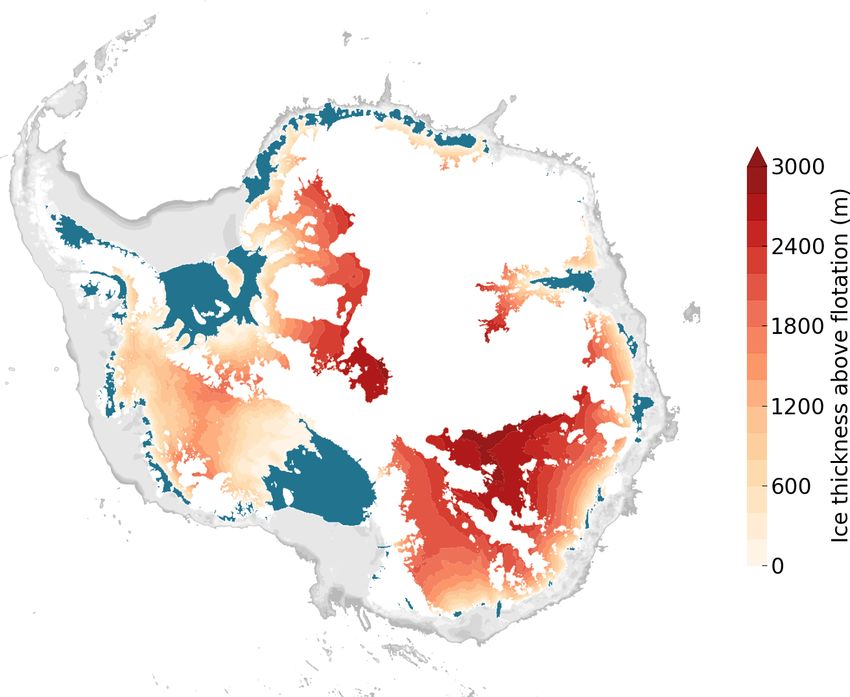
1624                                                        A. Levermann and J. Feldmann: Timescale of Antarctic instabilities

Figure 2. Scaling of bed geometry and maps of data involved in the response-time calculation (here shown exemplarily for Thwaites Glacier
– TG – with respect to the reference Pine Island Glacier – PIG). (a)–(b) Elevation of ice surface (grey) and bedrock (black) with retrograde
slope section (colored) that is used to infer the vertical scale and the slope magnitude for the transects shown in panels (d)–(g). Panel (c)
shows the bed geometry of the retrograde slope section, scaled with vertical and horizontal scaling factors (Table 1) and normalized to the
dimensions of Pine Island Glacier. Maps of (d) surface mass balance (van Wessem et al., 2014), (e) bed topography (Fretwell et al., 2013),
(f) surface velocity (Rignot et al., 2011) and (g) basal friction (Morlighem et al., 2013). Drainage basins are obtained from Zwally et al.
(2012). The transects as shown in panels (a) and (b) are provided as black and yellow lines in panels (d)–(g).

scaling ratio would indicate a faster response and the other             2.2   Data
a slower response compared to the reference). The second
criterion yields the relative error between the two calculated           The locations of the chosen transects are motivated by the
response-time ratios with respect to their mean and ensures              bed topography and the flow field of the analyzed outlets to
that this uncertainty is at most 20 %. Ice streams with a larger         capture their retrograde bed section directly upstream of the
uncertainty in their calculated time scaling are reported in the         grounding line (e.g., see Fig. 2). The ice-stream characteris-
following but considered to be unsuitable for the approach               tic parameter values are all obtained from datasets that rep-
used here.                                                               resent present-day conditions of the Antarctic Ice Sheet. The
                                                                         bed topography stems from the BEDMAP2 dataset (Fretwell
                                                                         et al., 2013), which is the most recent continent-wide compi-
                                                                         lation of Antarctic ice thickness and basal topography and in-
                                                                         volves data from various sources, including satellite, airborne

The Cryosphere, 13, 1621–1633, 2019                                                            www.the-cryosphere.net/13/1621/2019/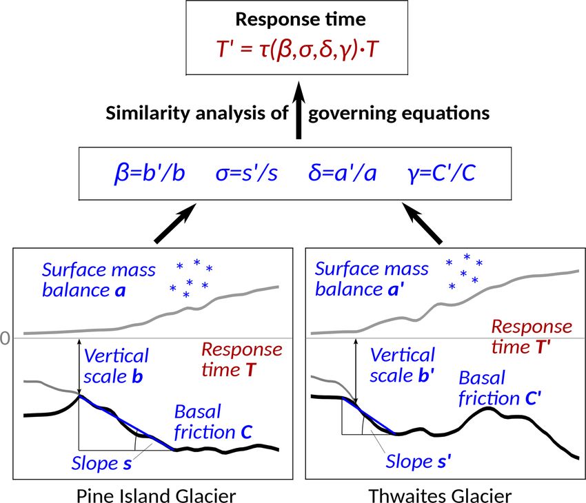
A. Levermann and J. Feldmann: Timescale of Antarctic instabilities 1625
radar, over-snow radar and seismic-sounding measurements
that total to 25 million data points. The basal-friction dataset
is taken from Morlighem et al. (2013) and is a product from
inversion of observed present-day Antarctic ice-surface ve-
locity (Rignot et al., 2011) with the Ice Sheet System Model
(Larour et al., 2012). The thermo-mechanical, higher-order
model uses anisotropic mesh refinement that allows for hor-
izontal resolutions down to 3 km along the Antarctic coast,
i.e., our region of interest. The field of basal friction is consis-
tent with results from other inversion models (Joughin et al.,
2009; Morlighem et al., 2010; Pollard and DeConto, 2012).
Surface mass balance is obtained from the Regional Atmo-
spheric Climate Model (RACMO version 2.3p2; van Wessem
et al., 2014) and is averaged over the period from 1979 to
2016. RACMO is forced by ERA-Interim reanalysis data at
the lateral boundaries, simulating the interaction of the ice
sheet with its atmospheric environment, involving relevant
processes such as solid precipitation, snow sublimation and
surface meltwater runoff. For most of the tributaries the sur-
face mass balance a is obtained from averaging over the en-
tire feeding catchment basin (Zwally et al., 2012). For some Figure 3. (a) Unscaled bed topography of retrograde slope sections
basins that have a long coastline and are drained by several of the six examined Antarctic outlets that fulfill the time-scaling cri-
major tributaries the averaging area is constrained to a region teria. (b) Bed topography from panel (a) scaled according to simili-
upstream of the ice stream of interest (Figs. S3–S6 and S9). tude theory using the horizontal and vertical length–scale ratios ob-
tained from observations (see Table 1) and normalized to the di-
mensions of the PIG slope (that has the same aspect ratio in both
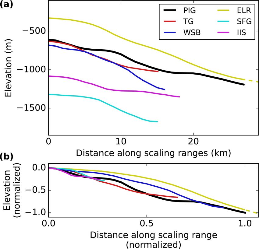
3 Results panels). For better visibility the x and y axis are cut (see Fig. S4 for
full extent of the ELR bed section).
The examined individual retrograde bed slopes vary in mag-
nitude by a factor of six and bed elevation differs by up to
1000 m (Figs. 3a and A2a). The lengths of the slope sections ranging from 46 % to 98 % (Table 1). Each of the discarded
indicate how far the considered retrograde slopes reach in- ice streams exhibits extremely slippery bed conditions, with
land before an (intermediate) section with vanishing slope basal-friction values of up to 3 orders of magnitude smaller
or an upsloping bed follows (Figs. 2 and S1–S9). We scale than the reference (Table 1). On the other hand these outlets
these bed sections with respect to the reference according to also have the smallest bed slopes of the ensemble. Both slope
the obtained vertical and horizontal length–scale ratios (Ta- and friction are hence subject to large relative uncertainties
ble 1). The resulting bed profiles collapse towards the refer- that mutually amplify in the calculation of τ and hence am-
ence showing similar downsloping while still exhibiting their plify the mismatch with e τ.
characteristic pattern (Figs. 3b and A2b). This confirms that Throughout the successfully examined outlets, diagnosed
the chosen geometric measures adequately reflect the char- basal friction and surface accumulation each differ by 1 or-
acteristics of the retrograde bed slopes. der of magnitude. Most slippery conditions and the highest
Within the ensemble of analyzed outlets TG has the small- snowfall are found in the Amundsen Sea sector, both favor-
est response time (Fig. 4), being 1.25 to almost 2 times as ing the short timescales of PIG and TG. We also infer the
fast as PIG, which is found to be the second fastest. For the scaling of the ice softness A using a third scaling law coming
chosen outlet of WSB the two calculated ratios indicate a out of the similarity analysis from Feldmann and Levermann
response that would be twice as slow as PIG. East Lambert (2016) (see Appendix A). The resulting ratios differ by two
Rift (ELR) and Institute Ice Stream (IIS) that feed Amery Ice orders of magnitude. For most of the ice streams discussed
Shelf and Filchner-Ronne Ice Shelf, respectively, are found here a lower softness value corresponds to a larger timescale.
to be 4 to 6 times slower than PIG. By far the slowest re- In other words, stiffer ice tends to slow down the response to
sponse is shown by Support Force Glacier (SFG), which is destabilization.
(more than) 10 times slower than PIG.
For each of these six tributaries (Table 1, bold) both im-
posed quality criteria (Eqs. 4 and 5) are fulfilled with a max-
imum error of c2 = 20 %. The other five regions are dis-
carded, since one or both of the criteria are not met, with c2
www.the-cryosphere.net/13/1621/2019/ The Cryosphere, 13, 1621–1633, 2019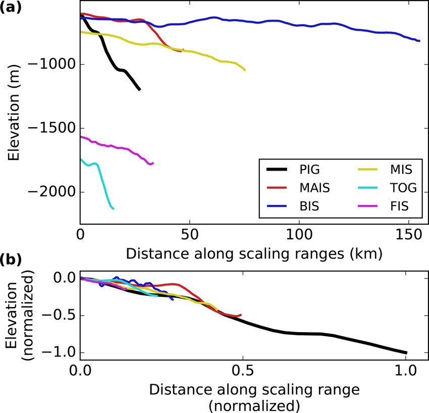
1626                                                            A. Levermann and J. Feldmann: Timescale of Antarctic instabilities

Table 1. Scaling ratios for all examined Antarctic outlets, clockwise, starting with the reference Pine Island Glacier. The ratios for the vertical
scale (β), the retrograde-slope magnitude (σ ), the basal friction (γ ) and the surface mass balance friction (δ) are inferred from observational
and model data (see Methods). The horizontal scaling ratio α, used for the scaling of the retrograde bed topography (Figs. 3 and A2), is
calculated via α = βσ −1 . The scaling of the ice softness ζ is obtained from Eq. (A2). The response-time ratios τ and e          τ are calculated
according to the scaling laws given by Eqs. (2) and (3). The last two columns show the resulting values from application of the two quality
criteria (Eqs. 4 and 5) according to which tributaries are either accepted (bold) or discarded.

          Tributary                                 α       β       σ          γ       δ         ζ        τ        τ
                                                                                                                   e         c1      c2
          Pine Island Glacier (PIG)                 1       1        1         1       1        1          1       1         1        1
          Thwaites Glacier (TG)                  0.86    1.03      1.2     0.77     1.28     1.72       0.53    0.81      0.42      0.2
          MacAyeal Ice Stream (MAIS)             3.54    0.99     0.28   0.0025     0.34    31.74       0.03    2.89     –1.96     0.98
          Bindschadler Ice Stream (BIS)          20.8    1.04     0.05   0.0029     0.34     0.79       1.13    3.04     15.47     0.46
          Mercer Ice Stream (MIS)                5.95    1.25     0.21     0.78     0.41     0.03      18.17    2.96      0.11     0.72
          Wilkes Subglacial Basin (WSB)          0.66    1.11     1.67     5.76     0.41     0.35       2.07    2.92      1.78     0.17
          Totten Glacier (TOG)                   2.37    2.84      1.2     0.22     0.53     0.29       0.15    6.04     –5.93     0.95
          East Lambert Rift (ELR)                0.41    0.54     1.31    10.15     0.16     1.08       5.93    4.03      0.62     0.19
          Support Force Glacier (SFG)            2.66    1.89     0.71      6.65     0.2     0.01      13.35    9.92      0.71     0.16
          Foundation Ice Stream (FIS)            8.83    2.56     0.29    0.036      0.2     0.14       0.43   13.16    –21.25     0.94
          Institute Ice Stream (IIS)             2.49    1.77     0.71      2.18    0.33     0.04       4.36    5.42      1.31     0.11

Figure 4. Map of inverse response time of Antarctic tributaries (two circles for each, corresponding to the two independent estimates, τ
and eτ ; see Table 1) relative to Pine Island Glacier (grey circle) as obtained from similitude analysis. Rectangles denote examined regions as
displayed in (Figs. 2 and S1–S9). Regions discarded from the analysis are shown in grey. Shown are (clockwise) Pine Island Glacier (PIG),
Thwaites Glacier (TG), MacAyeal Ice Stream (MAIS), Bindschadler Ice Stream (BIS), Mercer Ice Stream (MIS), Wilkes Subglacial Basin
(WSB), Totten Glacier (TOG), East Lambert Rift (ELR), Support Force Glacier (SFG), Foundation Ice Stream (FIS) and Institute Ice Stream
(IIS). Marine bed topography in blue (color bar), ice shelves in yellow and continental shelf in grey are taken from BEDMAP2 (Fretwell
et al., 2013).

The Cryosphere, 13, 1621–1633, 2019                                                                  www.the-cryosphere.net/13/1621/2019/
A. Levermann and J. Feldmann: Timescale of Antarctic instabilities 1627
4 Discussion single scale. This is realized by averaging spatially varying,
complex fields along a representative transect (ice softness
According to observations, PIG and TG have been showing and basal friction) or over the entire catchment basin (surface
the largest ice discharge rates in the Amundsen Sea Sector mass balance). While such an approach means a substantial
of West Antarctica since the last 4 decades, including phases idealization of the complex nature of ice dynamics, it allows
of rapid ice speed-up, dynamic thinning and grounding-line for a timescale analysis that is based on representative ice-
retreat (Rignot et al., 2014; Mouginot et al., 2014; Konrad property scales and considers the relevant physics through
et al., 2018). PIG’s most recent acceleration was found to the (simplified) stress balance. Our analysis will only be valid
coincide with the ungrounding of a region of only lightly as long as this representation is sufficient. We chose 11 out-
grounded ice, and the grounding line that is now at the up- let glaciers around Antarctica that we deem suitable for our
stream end of this area has been stabilizing during the last pragmatic method of collecting the required data along rep-
few years (Mouginot et al., 2014). Meanwhile PIG’s decel- resentative transects. Indeed, several more potentially MISI-
eration in ice discharge is more than compensated by TG’s prone Antarctic outlets exist, generally characterized by a
speed-up, which can be attributed to reduced ice-shelf but- curved shape. Their analysis would require a more sophis-
tressing that previously stabilized the upstream grounded ticated way of obtaining the data, e.g., along streamlines in-
ice (Rignot et al., 2014). It thus remains an open question stead of straight lines, which is not considered in this study.
whether the current destabilization of TG will result in re- Our approach assumes idealized conditions of unstable re-
treat rates larger than PIG’s recent retreat rates and hence treat. Though taking into account bed friction as a possible
confirm our finding of a faster timescale of TG compared stabilizing factor (Ritz et al., 2015) it is strongly limited by
to PIG. Regional model simulations of these regions (Favier not explicitly accounting for the stabilizing effect of ice-shelf
et al., 2014; Joughin et al., 2014) indicate that TG’s discharge buttressing (Dupont and Alley, 2005; Gudmundsson, 2013).
rate is up to a factor of 2 larger than PIG’s after the basal-melt That is, the approach estimates the timescale of retreat only
perturbation has ceased and the glaciers have relaxed into a after no significant ice shelf is present anymore or for the sit-
configuration of constant ice discharge. uation of an unconfined ice shelf that does not provide any
The relatively large timescales of SFG, IIS and ELR, backstress (e.g., as might be the case for the present-day TG
calculated here, are consistent with results from dynamical ice shelf; Rignot et al., 2014). Furthermore, our investigation
modeling that find these outlets of the Filchner-Ronne Ice is constrained to the short initial time period (decades to cen-
Shelf and Amery Ice Shelf to be far less sensitive to insta- turies) after destabilization, during which the grounding line
bility (Gong et al., 2014; Wright et al., 2014; Thoma et al., passes the investigated retrograde bed-slope section near the
2015; Ritz et al., 2015; Mengel et al., 2016) than WSB (Men- coast.
gel and Levermann, 2014) and PIG and TG (Favier et al., The used datasets of observed bed and ice geometry still
2014; Joughin et al., 2014; Feldmann and Levermann, 2015; show substantial gaps in coverage, though the regions an-
Seroussi et al., 2017). In these cases the buttressing effect alyzed here lie at the lower end of the uncertainty range
of the large ice shelves and the narrow, channel-type bed to- (Fretwell et al., 2013, their Figs. 11 and 12). Measurements
pography confining these outlets as well as relatively high of the Antarctic surface mass balance are in general sparsely
basal friction (Table 1) might prevent MISI initiation and distributed over the continent. In contrast, results from nu-
limit grounding-line retreat. merical modeling are known to have biases with respect to
Our results are obtained from the application of scal- observations. To reduce uncertainty we use a surface-mass-
ing laws, a procedure commonly pursued in hydrodynam- balance dataset obtained from a regional climate model that
ics and engineering (e.g., Scruton, 1961; Li et al., 2013) and was calibrated by the available observational data (van de
also to some extent in the field of glaciology (e.g., Burton Berg et al., 2006; van Wessem et al., 2014).
et al., 2012; Corti et al., 2014). The two scaling laws used
here (Eqs. 2 and 3) are derived from an approximation of
the Stokes stress balance (Feldmann and Levermann, 2016). 5 Conclusions
The approximation accounts for the dynamics of shallow ice
streams that are characterized by dominating longitudinal Combining observations and modeling data with a similarity
stresses and rapid sliding and typically have an onset at a analysis of the governing, simplified ice-dynamic equations
few 10 to 100 km upstream of the grounding line. Our analy- we apply the similitude principle (Fig. 1) to 11 MISI-prone
sis focuses precisely on such regions. The examined sections Antarctic outlets to infer their relative timescales (Fig. 4).
are all situated in the proximity of the grounding line and Assuming potential destabilization of these outlets (MISI
indeed exhibit slippery bed conditions and fast ice flow as triggered) in the absence of ice-shelf buttressing, our re-
indicated by inferred basal friction and velocity data, respec- sults suggest that PIG and TG have the smallest response
tively (Figs. 2, S1–S9f and g). time to destabilization (Fig. 4; Table 1), with TG respond-
The proposed method is based on the assumption that the ing between 1.25 to almost 2 times as fast as PIG. Further
ice-stream-specific properties can each be represented by a considered ice streams draining East or West Antarctica are
www.the-cryosphere.net/13/1621/2019/ The Cryosphere, 13, 1621–1633, 20191628 A. Levermann and J. Feldmann: Timescale of Antarctic instabilities found to respond twice (WSB) to 10 times (SFG) as slow as Data availability. The datasets related to this paper are available PIG. This also suggests that the dynamic regime of PIG is upon request from the authors. more similar to TG than to any other of the outlets analyzed here. This way, the proposed scaling approach may help field workers in their decision on which glaciers to observe to be able to study a broad and thus insightful spectrum of different (dissimilar) glacier dynamics. The presented analysis cannot make any statements about absolute timescales of the instabilities. It is constrained to relative statements between the different outlet glaciers based on their specific geometry and physical conditions, which carry information of the specific dynamic balance within the respective outlet glacier. Regarding absolute re- sponse times of individual tributaries, continued observation of the retreat of PIG and TG that extends the data that are al- ready available might allow deducing long-term trends, thus giving estimates for the absolute timescales of instability. These could be used to calibrate the method presented here. Our method comes with a large number of assumptions and limitations. Uncertainties will reduce as observational data further improve, and the relevance of the results will increase with sophistication of the method (e.g., explicit inclusion of ice-shelf buttressing). The Cryosphere, 13, 1621–1633, 2019 www.the-cryosphere.net/13/1621/2019/
A. Levermann and J. Feldmann: Timescale of Antarctic instabilities                                                                1629

Appendix A: Third independent scaling law

There is a third independent scaling law derived by similarity
analysis in Feldmann and Levermann (2016), coming out of
the viscous term of the SSA (see their Eqs. 9 and 12). Mak-
ing the common choice of Glen’s flow-law exponent n = 3
(Greve and Blatter, 2009), it reads

τ̄ = β −3 ζ,                                              (A1)

involving the ice-softness ratio ζ = A0 /A. Due the absence
of Antarctic ice-softness data, we cannot utilize this scaling
law to calculate a third independent timescale ratio. However,
combining this third scaling law (Eq. A1) with the first one
(Eq. 2), we eliminate the timescale ratio to calculate the ice-
softness ratio via

ζ = β −3 σ 2 γ −1 .                                       (A2)
                                                                  Figure A1. Ice thickness above flotation of marine regions (bedrock
Being dependent on the scaling of the geometry and the basal      below sea level) that are connected to the ocean (color bar). Ice
friction, ζ can be considered to be the ratio between ice-        shelves are in blue, and the continental shelf is in grey. Ice and bed
softness scales that are representative of the analyzed outlets   topography are taken from the BEDMAP2 compilation (Fretwell
cross sections (Table 1).                                         et al., 2013).

                                                                  Figure A2. Same as Fig. 3, but here for the five discarded Antarctic
                                                                  outlets.

www.the-cryosphere.net/13/1621/2019/                                                      The Cryosphere, 13, 1621–1633, 2019
1630 A. Levermann and J. Feldmann: Timescale of Antarctic instabilities
Supplement. The supplement related to this article is available Cook, S. J. and Swift, D. A.: Subglacial Basins: Their Origin and
online at: https://doi.org/10.5194/tc-13-1621-2019-supplement. Importance in Glacial Systems and Landscapes, Earth-Sci. Rev.,
115, 332–372, https://doi.org/10.1016/j.earscirev.2012.09.009,
2012.
Author contributions. AL designed the study. AL and JF carried Corti, G., Zeoli, A., and Iandelli, I.: Small-Scale Mod-
out the analysis and wrote the manuscript. JF prepared the figures. eling of Ice Flow Perturbations Induced by Sudden
Ice Shelf Breakup, Global Planet. Change, 119, 51–55,
https://doi.org/10.1016/j.gloplacha.2014.05.002, 2014.
Competing interests. The authors declare that they have no conflict DeConto, R. M. and Pollard, D.: Contribution of Antarctica
of interest. to Past and Future Sea-Level Rise, Nature, 531, 591–597,
https://doi.org/10.1038/nature17145, 2016.
Dupont, T. K. and Alley, R. B.: Assessment of the Impor-
tance of Ice-Shelf Buttressing to Ice-Sheet Flow: but-
Acknowledgements. We thank Mathieu Morlighem for providing
tressing sensitivity, Geophys. Res. Lett., 32, L04503,
the dataset of Antarctic basal friction. We are grateful to J. Mel-
https://doi.org/10.1029/2004GL022024, 2005.
chior van Wessem for providing the field of Antarctic surface mass
Favier, L., Gagliardini, O., Durand, G., and Zwinger, T.: A three-
balance. We thank Martin Lüthi and one anonymous reviewer for
dimensional full Stokes model of the grounding line dynamics:
their valuable and helpful comments and suggestions.
effect of a pinning point beneath the ice shelf, The Cryosphere,
6, 101–112, https://doi.org/10.5194/tc-6-101-2012, 2012.
Favier, L., Durand, G., Cornford, S. L., Gudmundsson, G. H.,
Financial support. This work was supported by the Deutsche Gagliardini, O., Gillet-Chaulet, F., Zwinger, T., Payne, A. J., and
Forschungsgemeinschaft (DFG) in the framework of the priority Le Brocq, A. M.: Retreat of Pine Island Glacier Controlled by
program “Antarctic Research with comparative investigations in Marine Ice-Sheet Instability, Nat. Clim. Change, 4, 117–121,
Arctic ice areas” by grant LE 1448/8-1. https://doi.org/10.1038/nclimate2094, 2014.
Feldmann, J. and Levermann, A.: Collapse of the West Antarc-
The publication of this article was funded by the tic Ice Sheet after Local Destabilization of the Amund-
Open Access Fund of the Leibniz Association. sen Basin, P. Natl. Acad. Sci. USA, 112, 14191–14196,
https://doi.org/10.1073/pnas.1512482112, 2015.
Feldmann, J. and Levermann, A.: Similitude of ice dynamics
Review statement. This paper was edited by Kenichi Matsuoka and against scaling of geometry and physical parameters, The
reviewed by Martin Lüthi and one anonymous referee. Cryosphere, 10, 1753–1769, https://doi.org/10.5194/tc-10-1753-
2016, 2016.
Fretwell, P., Pritchard, H. D., Vaughan, D. G., Bamber, J. L., Bar-
rand, N. E., Bell, R., Bianchi, C., Bingham, R. G., Blanken-
References ship, D. D., Casassa, G., Catania, G., Callens, D., Conway, H.,
Cook, A. J., Corr, H. F. J., Damaske, D., Damm, V., Ferracci-
Asay-Davis, X. S., Cornford, S. L., Durand, G., Galton-Fenzi, B. oli, F., Forsberg, R., Fujita, S., Gim, Y., Gogineni, P., Griggs,
K., Gladstone, R. M., Gudmundsson, G. H., Hattermann, T., Hol- J. A., Hindmarsh, R. C. A., Holmlund, P., Holt, J. W., Jacobel,
land, D. M., Holland, D., Holland, P. R., Martin, D. F., Mathiot, R. W., Jenkins, A., Jokat, W., Jordan, T., King, E. C., Kohler,
P., Pattyn, F., and Seroussi, H.: Experimental design for three J., Krabill, W., Riger-Kusk, M., Langley, K. A., Leitchenkov,
interrelated marine ice sheet and ocean model intercomparison G., Leuschen, C., Luyendyk, B. P., Matsuoka, K., Mouginot,
projects: MISMIP v. 3 (MISMIP +), ISOMIP v. 2 (ISOMIP +) J., Nitsche, F. O., Nogi, Y., Nost, O. A., Popov, S. V., Rignot,
and MISOMIP v. 1 (MISOMIP1), Geosci. Model Dev., 9, 2471– E., Rippin, D. M., Rivera, A., Roberts, J., Ross, N., Siegert,
2497, https://doi.org/10.5194/gmd-9-2471-2016, 2016. M. J., Smith, A. M., Steinhage, D., Studinger, M., Sun, B.,
Bamber, J. L., Riva, R. E. M., Vermeersen, B. L. A., and LeBrocq, Tinto, B. K., Welch, B. C., Wilson, D., Young, D. A., Xiangbin,
A. M.: Reassessment of the Potential Sea-Level Rise from a Col- C., and Zirizzotti, A.: Bedmap2: improved ice bed, surface and
lapse of the West Antarctic Ice Sheet, Science, 324, 901–903, thickness datasets for Antarctica, The Cryosphere, 7, 375–393,
https://doi.org/10.1126/science.1169335, 2009. https://doi.org/10.5194/tc-7-375-2013, 2013.
Bentley, C. R., Crary, A. P., Ostenso, N. A., and Thiel, Goldberg, D., Holland, D. M., and Schoof, C.: Ground-
E. C.: Structure of West Antarctica, Science, 131, 131–136, ing Line Movement and Ice Shelf Buttressing in
https://doi.org/10.1126/science.131.3394.131, 1960. Marine Ice Sheets, J. Geophys. Res., 114, F04026,
Buckingham, E.: On Physically Similar Systems; Illustrations of https://doi.org/10.1029/2008JF001227, 2009.
the Use of Dimensional Equations, Phys. Rev., 4, 345–376, Golledge, N. R., Kowalewski, D. E., Naish, T. R., Levy, R. H., Fog-
https://doi.org/10.1103/PhysRev.4.345, 1914. will, C. J., and Gasson, E. G. W.: The Multi-Millennial Antarctic
Burton, J. C., Amundson, J. M., Abbot, D. S., Boghosian, A., Cath- Commitment to Future Sea-Level Rise, Nature, 526, 421–425,
les, L. M., Correa-Legisos, S., Darnell, K. N., Guttenberg, N., https://doi.org/10.1038/nature15706, 2015.
Holland, D. M., and MacAyeal, D. R.: Laboratory Investigations Gong, Y., Cornford, S. L., and Payne, A. J.: Modelling the response
of Iceberg Capsize Dynamics, Energy Dissipation and Tsunami- of the Lambert Glacier–Amery Ice Shelf system, East Antarctica,
genesis: Iceberg capsize dynamics, J. Geophys. Res.-Earth, 117, to uncertain climate forcing over the 21st and 22nd centuries, The
F01007, https://doi.org/10.1029/2011JF002055, 2012.
The Cryosphere, 13, 1621–1633, 2019 www.the-cryosphere.net/13/1621/2019/A. Levermann and J. Feldmann: Timescale of Antarctic instabilities 1631 Cryosphere, 8, 1057–1068, https://doi.org/10.5194/tc-8-1057- Jenkins, A., Shoosmith, D., Dutrieux, P., Jacobs, S., Kim, 2014, 2014. T. W., Lee, S. H., Ha, H. K., and Stammerjohn, S.: West Greenbaum, J. S., Blankenship, D. D., Young, D. A., Richter, T. G., Antarctic Ice Sheet Retreat in the Amundsen Sea Driven Roberts, J. L., Aitken, A. R. A., Legresy, B., Schroeder, D. M., by Decadal Oceanic Variability, Nat. Geosci., 11, 733–738, Warner, R. C., van Ommen, T. D., and Siegert, M. J.: Ocean Ac- https://doi.org/10.1038/s41561-018-0207-4, 2018. cess to a Cavity beneath Totten Glacier in East Antarctica, Nat. Joughin, I. and Alley, R. B.: Stability of the West Antarctic Geosci., 8, 294–298, https://doi.org/10.1038/ngeo2388, 2015. Ice Sheet in a Warming World, Nat. Geosci., 4, 506–513, Greene, C. A., Blankenship, D. D., Gwyther, D. E., Sil- https://doi.org/10.1038/ngeo1194, 2011. vano, A., and van Wijk, E.: Wind Causes Totten Ice Shelf Joughin, I., Tulaczyk, S., Bamber, J. L., Blankenship, D., Holt, Melt and Acceleration, Science Advances, 3, e1701681, J. W., Scambos, T., and Vaughan, D. G.: Basal Conditions for https://doi.org/10.1126/sciadv.1701681, 2017. Pine Island and Thwaites Glaciers, West Antarctica, Determined Greve, R. and Blatter, H.: Dynamics of Ice Sheets and Glaciers, Using Satellite and Airborne Data, J. Glaciol., 55, 245–257, Advances in Geophysical and Environmental Mechanics and https://doi.org/10.3189/002214309788608705, 2009. Mathematics, Springer Berlin Heidelberg, Berlin, Heidelberg, Joughin, I., Smith, B. E., and Medley, B.: Marine Ice https://doi.org/10.1007/978-3-642-03415-2, 2009. Sheet Collapse Potentially Under Way for the Thwaites Gudmundsson, G. H.: Ice-shelf buttressing and the stabil- Glacier Basin, West Antarctica, Science, 344, 735–738, ity of marine ice sheets, The Cryosphere, 7, 647–655, https://doi.org/10.1126/science.1249055, 2014. https://doi.org/10.5194/tc-7-647-2013, 2013. Konrad, H., Shepherd, A., Gilbert, L., Hogg, A. E., McMil- Gudmundsson, G. H., Krug, J., Durand, G., Favier, L., and Gagliar- lan, M., Muir, A., and Slater, T.: Net Retreat of Antarc- dini, O.: The stability of grounding lines on retrograde slopes, tic Glacier Grounding Lines, Nat. Geosci., 11, 258–262, The Cryosphere, 6, 1497–1505, https://doi.org/10.5194/tc-6- https://doi.org/10.1038/s41561-018-0082-z, 2018. 1497-2012, 2012. Kundu, P., Cohen, I., and Hu, H.: Fluid Mechanics, Academic Press, Hellmer, H. H., Kauker, F., Timmermann, R., Determann, J., and New Delhi, 2012. Rae, J.: Twenty-First-Century Warming of a Large Antarctic Ice- Larour, E., Seroussi, H., Morlighem, M., and Rignot, E.: Conti- Shelf Cavity by a Redirected Coastal Current, Nature, 485, 225– nental Scale, High Order, High Spatial Resolution, Ice Sheet 228, https://doi.org/10.1038/nature11064, 2012. Modeling Using the Ice Sheet System Model (ISSM): ice Hillenbrand, C.-D., Smith, J. A., Hodell, D. A., Greaves, M., sheet system model, J. Geophys. Res.-Earth, 117, F01022, Poole, C. R., Kender, S., Williams, M., Andersen, T. J., Jer- https://doi.org/10.1029/2011JF002140, 2012. nas, P. E., Elderfield, H., Klages, J. P., Roberts, S. J., Gohl, K., Li, Y., Wu, M., Chen, X., Wang, T., and Liao, H.: Wind- Larter, R. D., and Kuhn, G.: West Antarctic Ice Sheet Retreat Tunnel Study of Wake Galloping of Parallel Cables on Cable- Driven by Holocene Warm Water Incursions, Nature, 547, 43– Stayed Bridges and Its Suppression, Wind Struct., 16, 249–261, 48, https://doi.org/10.1038/nature22995, 2017. https://doi.org/10.12989/was.2013.16.3.249, 2013. Huybrechts, P., Goelzer, H., Janssens, I., Driesschaert, E., Fichefet, Macagno, E. O.: Historico-Critical Review of Dimensional Anal- T., Goosse, H., and Loutre, M.-F.: Response of the Green- ysis, J. Franklin I., 292, 391–402, https://doi.org/10.1016/0016- land and Antarctic Ice Sheets to Multi-Millennial Green- 0032(71)90160-8, 1971. house Warming in the Earth System Model of Intermedi- MacAyeal, D. R.: Large-Scale Ice Flow over a Viscous ate Complexity LOVECLIM, Surv. Geophys., 32, 397–416, Basal Sediment: Theory and Application to Ice Stream https://doi.org/10.1007/s10712-011-9131-5, 2011. B, Antarctica, J. Geophys. Res.-Sol. Ea., 94, 4071–4087, The IMBIE team: Mass Balance of the Antarctic Ice https://doi.org/10.1029/JB094iB04p04071, 1989. Sheet from 1992 to 2017, Nature, 558, 219–222, Medley, B., Joughin, I., Smith, B. E., Das, S. B., Steig, E. J., https://doi.org/10.1038/s41586-018-0179-y, 2018. Conway, H., Gogineni, S., Lewis, C., Criscitiello, A. S., Mc- IPCC, WG I: Climate Change 2013: The Physical Science Basis. Connell, J. R., van den Broeke, M. R., Lenaerts, J. T. M., Contribution of Working Group I to the Fifth Assessment Report Bromwich, D. H., Nicolas, J. P., and Leuschen, C.: Constrain- of the Intergovernmental Panel on Climate Change, Cambridge ing the recent mass balance of Pine Island and Thwaites glaciers, University Press, Cambridge, United Kingdom and New York, West Antarctica, with airborne observations of snow accumula- NY, USA, 2013. tion, The Cryosphere, 8, 1375–1392, https://doi.org/10.5194/tc- IPCC, WG II: Climate Change 2014: Impacts, Adaptation, and Vul- 8-1375-2014, 2014. nerability, Part A: Global and Sectoral Aspects, Contribution of Mengel, M. and Levermann, A.: Ice Plug Prevents Irreversible Dis- Working Group II to the Fifth Assessment Report of the Inter- charge from East Antarctica, Nat. Clim. Change, 4, 451–455, governmental Panel on Climate Change, edited by: Field, C. B., https://doi.org/10.1038/nclimate2226, 2014. Barros, V. R., Dokken, D. J., Mach, K. J., Mastrandrea, M. D., Mengel, M., Feldmann, J., and Levermann, A.: Linear Sea- Bilir, T. E., Chatterjee, M., Ebi, K. L., Estrada, Y. O., Genova, R. Level Response to Abrupt Ocean Warming of Major C., Girma, B., Kissel, E. S., Levy, A. N., MacCracken, S., Mas- West Antarctic Ice Basin, Nat. Clim. Change, 6, 71–74, trandrea, P. R., and White, L. L., Cambridge University Press, https://doi.org/10.1038/nclimate2808, 2016. Cambridge, United Kingdom and New York, NY, USA, 2014. Mercer, J. H.: West Antarctic Ice Sheet and CO2 Green- Jenkins, A., Dutrieux, P., Jacobs, S. S., McPhail, S. D., Perrett, J. R., house Effect: A Threat of Disaster, Nature, 271, 321–325, Webb, A. T., and White, D.: Observations beneath Pine Island https://doi.org/10.1038/271321a0, 1978. Glacier in West Antarctica and Implications for Its Retreat, Nat. Geosci., 3, 468–472, https://doi.org/10.1038/ngeo890, 2010. www.the-cryosphere.net/13/1621/2019/ The Cryosphere, 13, 1621–1633, 2019
1632                                                         A. Levermann and J. Feldmann: Timescale of Antarctic instabilities

Morland, L. W.: Unconfined Ice-Shelf Flow, in: Dynamics of the          Ross, N., Bingham, R. G., Corr, H. F. J., Ferraccioli, F., Jordan,
   West Antarctic Ice Sheet, edited by: Van der Veen, C. J. and           T. A., Le Brocq, A., Rippin, D. M., Young, D., Blankenship,
   Oerlemans, J., Glaciology and Quaternary Geology, Springer             D. D., and Siegert, M. J.: Steep Reverse Bed Slope at the Ground-
   Netherlands, 99–116, 1987.                                             ing Line of the Weddell Sea Sector in West Antarctica, Nat.
Morlighem, M., Rignot, E., Seroussi, H., Larour, E., Ben Dhia,            Geosci., 5, 393–396, https://doi.org/10.1038/ngeo1468, 2012.
   H., and Aubry, D.: Spatial Patterns of Basal Drag In-                Schoof, C.: Ice Sheet Grounding Line Dynamics: Steady States,
   ferred Using Control Methods from a Full-Stokes and Sim-               Stability, and Hysteresis, J. Geophys. Res., 112, F03S28,
   pler Models for Pine Island Glacier, West Antarctica: spa-             https://doi.org/10.1029/2006JF000664, 2007.
   tial patterns of basal drag, Geophys. Res. Lett., 37, L14502,        Scruton, C.: Wind Tunnels and Flow Visualization, Nature, 189,
   https://doi.org/10.1029/2010GL043853, 2010.                            108–110, https://doi.org/10.1038/189108a0, 1961.
Morlighem, M., Seroussi, H., Larour, E., and Rignot, E.: In-            Seroussi, H., Nakayama, Y., Larour, E., Menemenlis, D.,
   version of Basal Friction in Antarctica Using Exact and In-            Morlighem, M., Rignot, E., and Khazendar, A.: Continued
   complete Adjoints of a Higher-Order Model: Antarctic basal             Retreat of Thwaites Glacier, West Antarctica, Controlled by
   friction inversion, J. Geophys. Res.-Earth, 118, 1746–1753,            Bed Topography and Ocean Circulation: Ice-ocean model-
   https://doi.org/10.1002/jgrf.20125, 2013.                              ing of thwaites glacier, Geophys. Res. Lett., 44, 6191–6199,
Mouginot, J., Rignot, E., and Scheuchl, B.: Sustained Increase in Ice     https://doi.org/10.1002/2017GL072910, 2017.
   Discharge from the Amundsen Sea Embayment, West Antarc-              Shean, D. E., Joughin, I. R., Dutrieux, P., Smith, B. E., and Berthier,
   tica, from 1973 to 2013, Geophys. Res. Lett., 41, 1576–1584,           E.: Ice shelf basal melt rates from a high-resolution DEM record
   https://doi.org/10.1002/2013GL059069, 2014.                            for Pine Island Glacier, Antarctica, The Cryosphere Discuss.,
Paolo, F. S., Fricker, H. A., and Padman, L.: Volume Loss from            https://doi.org/10.5194/tc-2018-209, in review, 2018.
   Antarctic Ice Shelves Is Accelerating, Science, 348, 327–331,        Smith, J. A., Andersen, T. J., Shortt, M., Gaffney, A. M., Truffer, M.,
   https://doi.org/10.1126/science.aaa0940, 2015.                         Stanton, T. P., Bindschadler, R., Dutrieux, P., Jenkins, A., Hillen-
Pattyn, F.: The Paradigm Shift in Antarctic Ice Sheet Modelling,          brand, C.-D., Ehrmann, W., Corr, H. F. J., Farley, N., Crowhurst,
   Nat. Commun., 9, 2728, https://doi.org/10.1038/s41467-018-             S., and Vaughan, D. G.: Sub-Ice-Shelf Sediments Record History
   05003-z, 2018.                                                         of Twentieth-Century Retreat of Pine Island Glacier, Nature, 541,
Pattyn, F., Ritz, C., Hanna, E., Asay-Davis, X., DeConto, R.,             77–80, https://doi.org/10.1038/nature20136, 2017.
   Durand, G., Favier, L., Fettweis, X., Goelzer, H., Golledge,         Szücs, E.: Fundamental Studies in Engineering II, Similitude
   N. R., Munneke, P. K., Lenaerts, J. T. M., Nowicki, S., Payne,         and Modeling, Elsevier Scientific Publishing Co., Amsterdam,
   A. J., Robinson, A., Seroussi, H., Trusel, L. D., and van den          Netherlands, 1980.
   Broeke, M.: The Greenland and Antarctic Ice Sheets under             Thoma, M., Determann, J., Grosfeld, K., Goeller, S., and
   1.5 ◦ C Global Warming, Nat. Clim. Change, 8, 1053–1061,               Hellmer, H. H.: Future Sea-Level Rise Due to Projected
   https://doi.org/10.1038/s41558-018-0305-8, 2018.                       Ocean Warming beneath the Filchner Ronne Ice Shelf: A
Pollard, D. and DeConto, R. M.: A simple inverse method                   Coupled Model Study, Earth Planet. Sc. Lett., 431, 217–224,
   for the distribution of basal sliding coefficients under ice           https://doi.org/10.1016/j.epsl.2015.09.013, 2015.
   sheets, applied to Antarctica, The Cryosphere, 6, 953–971,           Timmermann, R. and Hellmer, H. H.: Southern Ocean Warm-
   https://doi.org/10.5194/tc-6-953-2012, 2012.                           ing and Increased Ice Shelf Basal Melting in the Twenty-
Pritchard, H. D., Ligtenberg, S. R. M., Fricker, H. A., Vaughan,          First and Twenty-Second Centuries Based on Coupled Ice-
   D. G., van den Broeke, M. R., and Padman, L.: Antarctic Ice-           Ocean Finite-Element Modelling, Ocean Dynam., 63, 1011–
   Sheet Loss Driven by Basal Melting of Ice Shelves, Nature, 484,        1026, https://doi.org/10.1007/s10236-013-0642-0, 2013.
   502–505, https://doi.org/10.1038/nature10968, 2012.                  van de Berg, W. J., van den Broeke, M. R., Reijmer, C. H.,
Rayleigh: The Principle of Similitude, Nature, 95, 66–68,                 and van Meijgaard, E.: Reassessment of the Antarctic Sur-
   https://doi.org/10.1038/095066c0, 1915.                                face Mass Balance Using Calibrated Output of a Regional At-
Reynolds, O.: An Experimental Investigation of the Circum-                mospheric Climate Model, J. Geophys. Res., 111, D11104,
   stances Which Determine Whether the Motion of Water Shall              https://doi.org/10.1029/2005JD006495, 2006.
   Be Direct or Sinuous, and of the Law of Resistance in                van Wessem, J. M., Reijmer, C. H., Lenaerts, J. T. M., van de
   Parallel Channels, Philos. T. R. Soc. Lond., 174, 935–982,             Berg, W. J., van den Broeke, M. R., and van Meijgaard, E.: Up-
   https://doi.org/10.1098/rstl.1883.0029, 1883.                          dated cloud physics in a regional atmospheric climate model im-
Rignot, E., Mouginot, J., and Scheuchl, B.: Ice Flow                      proves the modelled surface energy balance of Antarctica, The
   of the Antarctic Ice Sheet, Science, 333, 1427–1430,                   Cryosphere, 8, 125–135, https://doi.org/10.5194/tc-8-125-2014,
   https://doi.org/10.1126/science.1208336, 2011.                         2014.
Rignot, E., Mouginot, J., Morlighem, M., Seroussi, H., and              Weertman, J.: Stability of the Junction of an Ice
   Scheuchl, B.: Widespread, Rapid Grounding Line Retreat of              Sheet and an Ice Shelf, J. Glaciol., 13, 3–11,
   Pine Island, Thwaites, Smith, and Kohler Glaciers, West Antarc-        https://doi.org/10.3189/S0022143000023327, 1974.
   tica, from 1992 to 2011, Geophys. Res. Lett., 41, 3502–3509,         Winkelmann, R., Levermann, A., Ridgwell, A., and Caldeira,
   https://doi.org/10.1002/2014GL060140, 2014.                            K.: Combustion of Available Fossil Fuel Resources Sufficient
Ritz, C., Edwards, T. L., Durand, G., Payne, A. J., Peyaud, V., and       to Eliminate the Antarctic Ice Sheet, Science Advances, 1,
   Hindmarsh, R. C. A.: Potential Sea-Level Rise from Antarctic           e1500589, https://doi.org/10.1126/sciadv.1500589, 2015.
   Ice-Sheet Instability Constrained by Observations, Nature, 528,
   115–118, https://doi.org/10.1038/nature16147, 2015.

The Cryosphere, 13, 1621–1633, 2019                                                           www.the-cryosphere.net/13/1621/2019/
A. Levermann and J. Feldmann: Timescale of Antarctic instabilities                                                                  1633

Wright, A. P., Le Brocq, A. M., Cornford, S. L., Bingham, R. G.,          Zwally, H. J., Giovinetto, M. B., Beckley, M. A., and Saba,
  Corr, H. F. J., Ferraccioli, F., Jordan, T. A., Payne, A. J., Rippin,     J. L.: Antarctic and Greenland Drainage Systems, GSFC
  D. M., Ross, N., and Siegert, M. J.: Sensitivity of the Weddell           Cryospheric Sciences Laboratory, available at: http://icesat4.
  Sea sector ice streams to sub-shelf melting and surface accumula-         gsfc.nasa.gov/cryo_data/ant_grn_drainage_systems.php (last ac-
  tion, The Cryosphere, 8, 2119–2134, https://doi.org/10.5194/tc-           cess: 1 May 2018), 2012.
  8-2119-2014, 2014.

www.the-cryosphere.net/13/1621/2019/                                                           The Cryosphere, 13, 1621–1633, 2019
You can also read