Whistler instability driven by the sunward electron deficit in the solar wind
←
→
Page content transcription
If your browser does not render page correctly, please read the page content below
Astronomy & Astrophysics manuscript no. main                                                                                       ©ESO 2021
                                                    July 23, 2021

                                                       Whistler instability driven by the sunward electron deficit in the
                                                                                   solar wind
                                                                                        High-cadence Solar Orbiter observations
                                                       L. Berčič1 , D. Verscharen1, 2 , C. J. Owen1 , L. Colomban3 , M. Kretzschmar3 , T. Chust4 , M. Maksimovic5 , D. O.
                                                      Kataria1 , C. Anekallu1 , E. Behar6, 7 , M. Berthomier4 , R. Bruno8 , V. Fortunato9 , C. W. Kelly1 , Y. V. Khotyaintsev10 ,
                                                                 G. R. Lewis1 , S. Livi11 , P. Louarn12 , G. Mele13 , G. Nicolaou11 , G. Watson1 , and R. T. Wicks14
arXiv:2107.10645v1 [physics.space-ph] 22 Jul 2021

                                                           1
                                                               Mullard Space Science Laboratory, University College London, Dorking, RH5 6NT, UK
                                                           2
                                                               Space Science Center, University of New Hampshire, 8 College Road, Durham NH 03824, USA
                                                           3
                                                               LPC2E/CNRS, 3 Avenue de la Recherche Scientifique, 45071 Orléans Cedex 2, France
                                                           4
                                                               LPP, CNRS, Ecole Polytechnique, Sorbonne Université, Observatoire de Paris, Université Paris-Saclay, Palaiseau, Paris, France
                                                           5
                                                               LESIA, Observatoire de Paris, Université PSL, CNRS, Sorbonne Université, Univ. Paris Diderot, Sorbonne Paris Cité, 5 place
                                                               Jules Janssen, 92195 Meudon, France
                                                           6
                                                               Swedish Institute of Space Physics (IRF), Kiruna, Sweden
                                                           7
                                                               Laboratoire Lagrange, OCA, UCA, CNRS, Nice, France
                                                           8
                                                               INAF-IAPS, Via Fosso del Cavaliere 100, 00133 Roma, Italy
                                                           9
                                                               Planetek Italia, Italy
                                                          10
                                                               Swedish Institute of Space Physics (IRF), Uppsala, Sweden
                                                          11
                                                               Southwest Research Institute, San Antonio, Texas, USA
                                                          12
                                                               IRAP, Université de Toulouse, CNRS, UPS, CNES, Toulouse, France
                                                          13
                                                               Leonardo, Taranto, Italy
                                                          14
                                                               Department of Mathematics, Physics and Electrical Engineering, Northumbria University, Newcastle upon Tyne, UK

                                                         Received March 31, 2021; accepted April 15, 2021

                                                                                                                     ABSTRACT

                                                         Context. Solar wind electrons play an important role in the energy balance of the solar wind acceleration by carrying energy into
                                                         interplanetary space in the form of electron heat flux. The heat flux is stored in the complex electron velocity distribution functions
                                                         (VDFs) shaped by expansion, Coulomb collisions, and field-particle interactions.
                                                         Aims. We investigate how the suprathermal electron deficit in the anti-strahl direction, which was recently discovered in the near-Sun
                                                         solar wind, drives a kinetic instability and creates whistler waves with wave vectors that are quasi-parallel to the direction of the
                                                         background magnetic field.
                                                         Methods. We combine high-cadence measurements of electron pitch-angle distribution functions and electromagnetic waves provided
                                                         by Solar Orbiter during its first orbit. Our case study is based on a burst-mode data interval from the Electrostatic Analyser System
                                                         (SWA-EAS) at a distance of 112 RS (0.52 au) from the Sun, during which several whistler wave packets were detected by Solar
                                                         Orbiter’s Radio and Plasma Waves (RPW) instrument.
                                                         Results. The sunward deficit creates kinetic conditions under which the quasi-parallel whistler wave is driven unstable. We directly
                                                         test our predictions for the existence of these waves through solar wind observations. We find whistler waves that are quasi-parallel
                                                         and almost circularly polarised, propagating away from the Sun, coinciding with a pronounced sunward deficit in the electron VDF.
                                                         The cyclotron-resonance condition is fulfilled for electrons moving in the direction opposite to the direction of wave propagation,
                                                         with energies corresponding to those associated with the sunward deficit.
                                                         Conclusions. We conclude that the sunward deficit acts as a source of quasi-parallel whistler waves in the solar wind. The quasilinear
                                                         diffusion of the resonant electrons tends to fill the deficit, leading to a reduction in the total electron heat flux.
                                                    1. Introduction                                                           collisions. Two suprathermal populations exist at higher ener-
                                                                                                                              gies: the strahl, which represents electrons typically stream-
                                                    The thermal energy of the solar corona is sufficient to accelerate        ing away from the Sun along the magnetic field, and the halo
                                                    part of its plasma into interplanetary space and create the solar         present at all pitch angles. The relative drifts of these popula-
                                                    wind. The solar wind consists mainly of protons, which carry the          tions must ensure the zero-current condition in the proton-rest
                                                    solar wind mass and momentum flux, and electrons, which carry             frame: nc vc + n s v s + nh vh = 0, where n j are the densities and v j
                                                    the solar wind heat flux.                                                 are the bulk velocities of the core ( j = c), strahl ( j = s), and halo
                                                        The heat flux is measured as the skewness (i.e., the third            ( j = h) (Feldman et al. 1975; Schwartz & Marsch 1983; Pilipp
                                                    moment) of the electron velocity distribution function (VDF),             et al. 1987; Maksimovic et al. 1997, 2005; Štverák et al. 2008;
                                                    which evolves with radial distance. The electron VDF typi-                Štverák et al. 2009; Tao et al. 2016).
                                                    cally consists of three separate populations. Most of the elec-
                                                    trons (more than 90%) belong to the core population which is                  Different models to capture the properties of the three elec-
                                                    present at low electron energies and dominated by Coulomb                 tron populations have been proposed in the past, often chosen
                                                                                                                                                                         Article number, page 1 of 12
A&A proofs: manuscript no. main
based on the capability of the data set used, and the needs in term 2019; Verscharen et al. 2019a; Agapitov et al. 2020; Micera et al.
of research goals (e.g. Štverák et al. 2009; Horaites et al. 2018; 2020). Oblique whistlers were recently observed in the near-Sun
Berčič et al. 2020). The core electrons are often represented by solar wind (Agapitov et al. 2020; Cattell et al. 2021b) and as-
a bi-Maxwellian distribution oriented with respect to the mag- sociated with enhanced strahl pitch-angle widths (Cattell et al.
netic field. Other models include, for example, bi-κ distributions 2021a).
and bi-self-similar distributions, which better describe the core We propose a resonant instability mechanism that creates
electrons observed by the Wind spacecraft in the vicinity of in- quasi-parallel whistler waves through the relaxation of the sun-
terplanetary shocks at 1 au (Wilson et al. 2019a,b). ward deficit in the core energy range in section 2. In Section 3
Recent observations of the near-Sun solar wind by Parker we describe the analysis of the high-cadence electron VDFs and
Solar Probe reveal a departure from the Maxwellian fit for the electromagnetic waves measured by Solar Orbiter. In Section 4
core population in the shape of a sunward deficit. This deficit is we display the observational results and relate them to the pro-
aligned with the magnetic field and located in the direction op- posed instability mechanism. In section 5 we discuss how our
posite to the strahl / heat flux in velocity space (Halekas et al. prediction corresponds to the data and existing studies and sum-
2020, 2021b,a; Berčič et al. 2020; Berčič et al. 2021). Halekas marise our findings.
et al. (2021b) show that the deficit makes a significant contribu-
tion to the total electron heat flux. 2. The quasi-parallel whistler instability driven by
Exospheric models of the solar wind describe the accelera- the sunward deficit
tion of the solar wind as the result of the ambipolar diffusion
of protons and electrons in an atmosphere that transitions from Recent in situ solar wind observations indicate that core elec-
collisional to collisionless conditions at the exobase. The elec- trons with energies larger than ∼ 2 wck depart from a traditional
trons are, due to their smaller mass, much more mobile than the bi-Maxwellian model, and exhibit a deficit in the direction op-
protons. This creates an ambipolar electric field which assures posite to the heat flux (Halekas et al. 2020, 2021b,a; Berčič et al.
the equality of electron and proton fluxes. In exospheric mod- 2020; Berčič et al. 2021). We investigate whether the sunward
els, the electron VDF consists of a highly anisotropic core and a deficit in the electron VDF can drive whistler waves unstable,
very narrow strahl, separated in energy by the ambipolar poten- and release its free energy through the growth of electromangetic
tial energy. In the sunward direction, the electron core exhibits fluctuations.
an abrupt cutoff defined by the ambipolar potential (Lemaire & One mechanism that allows an energy exchange between
Scherer 1970, 1971; Jockers 1970; Maksimovic et al. 1997; Pier- particles and fields are the resonant interactions between parti-
rard et al. 1999; Zouganelis et al. 2004). cles and waves. These interactions are characterised by a res-
Observations differ from these predictions of collisionless onance condition. In the case of parallel-propagating whistler
exospheric models. For example, solar wind core electrons are waves with frequency ω and wavenumber kk , the resonance con-
often quasi-isotropic, the strahl is substantially scattered towards dition is (e.g. Sagdeev & Galeev 1969; Marsch 2006; Shklyar &
larger pitch angles, and a second suprathermal population, the Matsumoto 2009)
halo, is present. The differences between the predicted and ob- ω − ωce
vk = vcyclo ≡ , (1)
served VDFs are attributed to the effects of Coulomb collisions kk
and field-particle interactions. Coulomb collisions are efficient in
where ωce = eB/me is the electron gyrofrequency, B is the mag-
isotropising the core population (Lie-Svendsen et al. 1997; Pier-
netic field, and me is the electron mass. Only electrons with the
rard et al. 2001; Salem et al. 2003; Smith et al. 2012; Štverák parallel velocity component vk = vcyclo undergo resonant in-
et al. 2008) as well as scattering the strahl at low electron en- teractions. Landau-resonant or higher-order cyclotron-resonant
ergies (Horaites et al. 2018, 2019; Boldyrev & Horaites 2019; interactions are not accessible for parallel-propagating whistler
Berčič et al. 2021). At higher energies, where collisions are rare, waves (e.g. Sagdeev & Galeev 1969; Verscharen et al. 2019b).
kinetic instabilities can reduce the skewness of electron VDF Quasi-parallel whistler waves are circular, purely right-hand
(Hollweg 1974; Gary et al. 1975; Feldman et al. 1976; Lakhina polarised waves with frequencies ω < ωce . Therefore, vcyclo < 0
1977; Krafft et al. 2005; Saito & Gary 2007). if ω/kk > 0 and vice versa according to Eq. (1). This means that
Resonant, electron-driven instabilities typically create waves the resonant electrons must move in the direction opposite to the
with frequencies between the ion and electron gyrofrequency. wave phase speed.
Enhanced fluctuations in this frequency band in the solar wind If electrons fulfil the resonance condition in Eq. (1), they fol-
often correspond to whistler waves. The most common observed low diffusion paths according to quasilinear theory. These diffu-
type of whistler waves are right-hand polarised, quasi-parallel sion paths correspond to curves of constant kinetic energy in the
whistler waves (Lacombe et al. 2014; Tong et al. 2019; Jagar- wave rest frame. The ambiguity in the direction of the quasilin-
lamudi et al. 2020, 2021). Zhang et al. (1998); Stansby et al. ear diffusion is resolved by the requirement that the diffusion is
(2016) and Kretzschmar et al. (2021) further find that the major- always directed from higher phase-space density to lower phase-
ity of the detected waves propagate in the anti-sunward direction. space density (Shapiro & Shevchenko 1963; Kennel & Engel-
These waves only resonate with electrons through the cyclotron mann 1966; Marsch 2006; Shklyar & Matsumoto 2009; Ver-
resonance, which is fulfilled by electrons moving in the oppo- scharen et al. 2019a).
site direction of the wave phase speed along the magnetic field. The instability mechanism is the same as for the Whistler
Whistler waves of this type cannot contribute to the scattering of Heat Flux Instability (WHFI) proposed by Gary et al. (1975):
the strahl electrons (Verscharen et al. 2019a). the key ingredient are the gradients of the distribution function in
Less frequently observed sunward whistler waves may be velocity space. However, in the classical derivation of the WHFI,
present in the solar wind, but obscured by turbulent fluctua- these gradients are produced by the relative drift between two
tions (Vasko et al. 2020; Vocks 2012). Oblique whistler waves, electron populations (e.g. the core and the halo). In our case, the
are also able to interact with strahl electrons and scatter them pitch angle gradient (∂ f /∂α) is a result of the local shape of the
through the strahl-driven oblique whistler instability (Vasko et al. distribution at the resonant speed.
Article number, page 2 of 12L. Berčič et al.: Whistler instability driven by the sunward electron deficit
Fig. 1 (b) shows the case in which the sunward deficit at
(a) v∥ (b) v∥ vk < 0 creates conditions for the diffusion towards smaller v⊥ ,
due to the change in the sign of ∂ f /∂α at vk = vcyclo . Electrons
strahl following the indicated diffusion paths lose kinetic energy. This
kinetic energy is transferred into the resonant whistler waves,
and causes the waves to grow. Case (b) thus illustrates the insta-
bility mechanism of the quasi-parallel whistler instability driven
by the sunward electron deficit in the anti-strahl direction.
We predict that this resonant wave–particle mechanism oc-
core curs in the solar wind. If this prediction is valid, we antici-
pate a correlation between the presence of quasi-parallel whistler
waves and the presence of increased sunward deficits in the elec-
vph tron VDFs. Our aim is to test this prediction with data from Solar
v⊥ Orbiter.
vc∥
3. Data Analysis Methods
wc 3.1. Solar wind electrons
vcyclo We present in-situ measurements from the first cruise-phase orbit
of Solar Orbiter (SO), the latest heliospheric mission designed
to link the solar wind to the plasma conditions at its origin in
the solar corona (Müller et al. 2020). Solar-wind electrons are
measured by the Electrostatic Analyser System (EAS) on board
Fig. 1. A schematics of the whistler instability driven by the sunward SO, consisting of two top-hat analyser heads, EAS 1 and EAS 2.
deficit in the anti-strahl direction. The core population is shown as a EAS is part of the Solar Wind Analyser (SWA) instrument suite,
blue shaded semi-circle, with a blue semi-circle marking its thermal ve- which also includes the Proton-Alpha Sensor (PAS), and the
locity (wc ) and vck its bulk velocity in plasma rest frame. The dashed Heavy Ion Sensor (HIS) characterising the solar-wind ion popu-
yellow curve indicates the strahl. Pink semi-circles mark curves of con-
stant energy in the rest frame of the wave moving with v ph = ω/kk , and
lations (Owen et al. 2020). SO’s fluxgate magnetometer (MAG)
black dashed semi-circles the curves of constant kinetic energy in the measures the magnetic field with a cadence of 8 Hz (Horbury
plasma frame. Pink arrows indicate the electron diffusion paths. (a) Ex- et al. 2020), while a search-coil magnetometer and electric field
ample without the sunward deficit; (b) The sunward deficit can trigger antennas, belonging to the Radio and Plasma Waves (RPW) in-
an instability. strument (Maksimovic et al. 2020), cover the higher-frequency
magnetic and electric field fluctuations.
Each of EAS’s instrument heads measures electron inflow
The schematic in Fig. 1 illustrates the quasilinear diffusion directions through 32 azimuth anodes with an angular width of
of electrons in the energy range corresponding to the observed 11.25◦ and 16 elevation deflector states with slightly variable an-
sunward deficit. We show two cases: (a) where electron core is gular widths of ∼ 3 − 10◦ . The EAS heads are positioned at the
represented by a bi-Maxwellian distribution, and (b) where this end of the spacecraft main boom, forming a combined field of
distribution exhibits a deficit at vk < 0. view (FOV) which covers almost the full solid angle of 4π. The
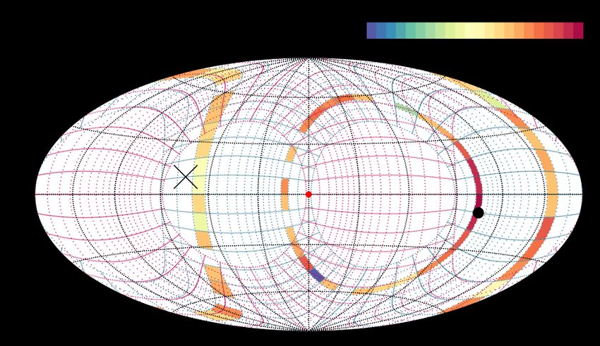
instrument’s FOV is presented in Fig. 2 with a skymap plot in the
The whistler wave assumed in this illustration propagates spacecraft (SC) reference frame. In this frame, the X-axis is the
with vph = ω/kk > 0 in the direction of the strahl electrons. It longitudinal axis of SO, pointing in the sunward direction, the
can resonate with the anti-strahl directed electrons with velocity Y-axis is the transverse azimuthal SC axis, and the Z-axis is or-
close to vcyclo according to Eq. (1) and marked in the figure. The thogonal to the two axes and pointing northward. The blue grid
curves of constant energy in the wave frame are shown in pink, describes the angular bins of EAS 1, and the red grid describes
and the curves of constant energy in the plasma frame in black. the angular bins of EAS 2. While some parts of the sky are cov-
The pink arrows describe the direction of the diffusion paths. ered by only one of the two heads, the FOVs of EAS 1 and EAS
These diffusion paths are always directed along the pink semi- 2 overlap in a large region.
circles of constant energy in the wave frame for the given vph of One electron energy sweep is conducted in 64 exponentially
the resonant waves. At the same time, the diffusion paths point spaced steps, detecting electrons with energies up to 5 keV, with
into the direction opposite to the pitch-angle gradient (−∂ f /∂α). a relative energy resolution of ∆E/E = 0.135. A full 3D dis-
In panel (a) of Fig. 1, this setup leads to a diffusion of resonant tribution scan is obtained within 0.92 ms, however downlinked
electrons from smaller to larger v⊥ . Electrons following these with a much lower cadence due to the limited available teleme-
diffusion paths gain kinetic energy in the plasma frame, which try budget (in Normal Mode (NM) every 10 s or 100 s).
must be provided from the assumed whistler wave. The wave In this work, we present electron VDFs measured in the in-
amplitude thus decreases, corresponding to wave damping. A strument’s Burst Mode (BM) at a cadence of 0.125 s. This higher
resonant wave–particle interaction of this type in which energy time resolution is made possible by a new operational concept,
is transferred from the waves to the electrons was studied with applied for the first time on SO (Owen et al. 2020; Owen, C. J.
a test-particle approach by Behar et al. (2020). This work finds et al. 2021). Assuming that the measured electron VDFs are gy-
that a deficit is created in the electron VDF near vk . vcyclo (see rotropic, a 3D VDF can be fully described by a 2D VDF in the
Fig. 4 by Behar et al. 2020). The electrons migrating from this magnetic field aligned frame. Removing one dimension substan-
phase-space region diffuse along the semi-circle and create an tially reduces the VDF data volume and thus the measurement
overdensity at larger pitch-angles with vk & vcyclo . time, as sampling of all perpendicular directions to the magnetic
Article number, page 3 of 12A&A proofs: manuscript no. main
the magnetic field used by EAS on-board is close to the ground
calibrated values. Strahl electrons, seen as a localised increase in
electron flux, follow the magnetic field azimuth angle.
We fit our electron VDFs with a bi-Maxwellian function to
obtain the electron core properties. Since the PAS sensor was
not operating on the chosen day, we perform fits in the EAS
magnetic-field aligned frame. We allow for a relative drift vck in
our bi-Maxwellian distribution in the direction parallel to mag-
netic field. The bi-Maxwellian distribution is given by
v⊥ (vk − vck )2
fc (v⊥ , vk ) = Ac exp − 2 − , (2)
wc⊥ w2ck
where Ac is the normalisation factor, wc⊥ is the perpendicular
Fig. 2. A skymap representation of the combined EAS FOV in the core thermal velocity, wck is the parallel core thermal velocity,
spacecraft (SC) reference frame. The centre of the plot is aligned with and vck is the core parallel drift velocity. These quantities are
the X-axis, 90◦ in longitude with the Y-axis, and latitude corresponds our fit parameters, from which we obtain the core parallel and
to the Z-axis. The angular bins are shown in blue for EAS 1 and in
perpendicular temperatures as
red for EAS 2. Two elevation bins of the EAS 1 head are filled with
data obtained during one scan in the instrument Burst Mode (BM). The
magnetic field direction is marked with a black dot (+B) and a black me w2ck me w2c⊥
cross (−B).
T ck = and T c⊥ = (3)
2kB 2kB
and the core density as
field is omitted. Therefore, before the start of each measurement
sequence, SWA receives the information about the current mag- nc = Ac π3/2 w2c⊥ wck . (4)
netic field vector from MAG. The instrument then defines the
EAS head as well as the appropriate elevation deflection states In the equation above, kB stands for the Boltzmann constant and
that sample the positive and negative magnetic field directions. me for the electron mass.
The energy sweep is then only performed in the two selected To improve the signal-to-noise ratio, we perfom our fits on
deflection states, for which EAS obtains all azimuth directions a moving window of two consecutive 2-dimensional gyrotropic
simultaneously. This procedure repeats every 0.125 s, produc- BM VDFs. We use a least-square minimisation algorithm2 pro-
ing the second-fastest electron pitch-angle distribution measure- vided by the Scipy Optimization package for Python (Virtanen
ments on any space mission to date, after the Fast Plasma Investi- et al. 2019). Because the VDF values span over several orders
gation (FPI) instrument on-board the Magnetospheric Multiscale of magnitude, we carry out our fits in logarithmic space (ln( fc )).
(MMS) spacecraft (Burch et al. 2016). A detailed description of This technique decreases the large difference in the weight of the
the instrument design and operating modes is given by Owen fitted data points. We use only energy bins between 15.3 eV and
et al. (2020). The BM operation and first results are presented by 107.2 eV to isolate the core population from the secondary elec-
Owen, C. J. et al. (2021). trons at lower energies and from the halo population at higher
We show an example of a BM scan in Fig. 2. We indicate the energies. We avoid the inclusion of strahl electrons by excluding
positive magnetic field direction with a black dot, and the nega- all data points within 30◦ pitch angle.
tive magnetic field direction with a black cross. For this case, the We normalise the core density obtained from the fit to the
data are collected by EAS 1 with the 3rd and the 14th elevation electron density obtained from the quasi-thermal-noise (QTN)
deflection states. Around the positive magnetic field direction, technique derived from the plasma peak in the electric field
the increased flux represents strahl electrons. power spectra (Meyer-Vernet et al. 2017, and references therein)
Even though magnetic field measurements are calibrated on- from RPW (Maksimovic et al. 2020). This technique gives an
board before being used by EAS, some differences occur be- accurate estimation of the electron density, which is limited in
tween the on-board and the on-ground calibrated magnetic-field precision by discrete sampling frequency bins and time resolu-
data. For our analysis, we use 8 Hz magnetic field measurements tion. The average value of the total electron density during the
from MAG which have been recalibrated on-ground and are pub- presented time interval is 19 cm−3 with an accuracy of 10 %.
licly available as L2 files on the SO archive1 . We fit the electron halo population using the same technique
We present the case study based on one time interval of just as described for the core. Due to the smaller signal-to-noise ratio
over 2 min duration of BM data from June 24, 2020. We choose in the halo energy range, we chose to fit the halo with a non-
this time period because of the good quality of the EAS data – drifting Maxwellian, even though small drifts along the magnetic
high electron counts and good correlation between the on-board field direction in the plasma rest frame have been found in the
and on-ground magnetic fields – and the presence of a clear sig- past (Štverák et al. 2009). With one fitting parameter less than in
nal of whistler waves in the associated RPW data. The evolution the core case, the probability for a successful fit increases and the
of the electron VDF sampled in each of the two selected eleva- noise in the obtained halo temperatures (T h⊥ , T hk ) decreases. We
tion bins is shown in the first two panels of Fig. 3 as a function of fit the halo to the difference between the observed VDF and the
the instrument azimuth angle and time. The third panel shows the core fit, fh = f − fc , limited to the energy range between 162.8 eV
corresponding elevation angles compared to the magnetic field and 655.2 eV. Measurements with pitch angles less than 30◦ are
direction. From the alignment between the magnetic-field direc- excluded to avoid the inclusion of the strahl electron population.
tion and the automatically chosen elevation bin, we conclude that
2
scipy.optimize.leastsq (https://docs.scipy.org/doc/scipy/
1
http://soar.esac.esa.int/soar/#home reference/generated/scipy.optimize.leastsq.html)
Article number, page 4 of 12L. Berčič et al.: Whistler instability driven by the sunward electron deficit
16 17
Fig. 3. Time evolution of BM data in the instrument frame. The top two panels show the electron VDFs as functions of time and the EAS 1 azimuth
angle for both of the selected elevation deflection states with a logarithmic colour scale. The bottom panel shows the sampled elevation angles.
Black lines in all plots denote the direction of the magnetic field in the EAS 1 frame.
2020 06 24 - 06:05:20.625 recorded waveforms; however, due to their large size, full wave
3 -6 forms can only be downlinked for short periods of time. A com-
13
f(s m ) plete overview of the wave activity at all times is assured by the
nc = 20.2 cm-3 10
spectral data product called Basic Parameters (BP), providing
Tc∥ = 20.1 eV
Tc⊥ = 18.4 eV core wave properties calculated on-board from time-averaged spectral
vc∥ = 27 kms-1 14
matrices (ASM). In the present study, we only use the follow-
10 strahl
nh = 1.5 cm-3
ing wave parameters derived from the SCM measurements: the
Th∥ = 145.8 eV halo magnetic trace power spectrum, the degree of polarization, the
Th⊥ = 147.6 eV
wave ellipticity, and the wave normal vector. We also present the
15
10 normalised electric-field power spectrum measured by RPW’s
electric-field antennas. Chust, T. et al. (2021) provide a detailed
description of the BP data products as well as a comparison of
10 16 these reduced products with the full waveform data.
RPW also provides a snapshot waveform (SWF) data prod-
uct during the selected period. SWF data consist of three times
2048 samples of magnetic and electric field fluctuations, avail-
10 17
15000 10000 5000 0 5000 10000 15000 able at different cadence (at best, every 22 s, but here ev-
v (km/s) ery 5 min), acquired at three different sampling frequencies:
24 576 Hz, 4096 Hz, and 256 Hz. Whistler mode waves exhibit
Fig. 4. Example of an electron VDF integrated over two consecutive
BM scans used for the core electron fit. Blue and red dots represent par-
frequencies of order a few 10 Hz, thus we investigate the 256 Hz
allel and perpendicular cuts through the electron VDF, while the two measurements consisting of an 8 s-long waveform interval be-
curves show the core and the halo fits. The velocity is given in the in- tween 06:05:11.5 and 06:05:19.5.
strument frame of reference and in the direction along the magnetic We identify frequency bands corresponding to the localised
field. enhancements in the magnetic-field power spectra, which are
characteristic for waves driven by kinetic instabilities. We per-
3.2. Electromagnetic fluctuations form a minimum-variance analysis of the bandpass-filtered data
to obtain the wave normal vector n̂. In our data intervals, the
Electromagnetic fluctuations are measured by the RPW triaxal identified waves are circularly polarised, and their wavevector is
coplanar electric antenna system (ANT), its biasing unit (BIAS), almost aligned with the magnetic field (i.e., quasi-parallel propa-
and a triaxal search-coil magnetometer (SCM) (Jannet et al. gation). The actual direction of propagation along n̂ must be de-
2021). Their common, most exhaustive data product includes the termined by considering the electric field measurements. Kret-
Article number, page 5 of 12A&A proofs: manuscript no. main
zschmar et al. (2021) show that the overwhelming majority of We show the time evolution of the BM electron VDF through
whistler waves observed by SO propagate in the anti-sunward pitch-angle distributions (PADs) averaged over different electron
direction and exhibit a "weak" phase deviation of 50◦ between energies in Fig. 7. In the lowest energy range, 50 - 100 eV, we ob-
the magnetic and electric field fluctuations that needs to be cor- serve two features in the parallel and anti-parallel directions with
rected. Applying this same correction here confirms the anti- respect to the magnetic field, while for higher energies only one
sunward wave propagation. of the features – the strahl electrons – remains. In order to com-
Due to the lack of PAS data, we cannot directly transform pensate for the noise in single electron-VDF measurements, we
the observed wave frequency from the SC frame to the plasma integrate the VDFs over selected time periods during which the
frame. The angle between the magnetic field vector and the ra- PADs are similar. We show these integrated VDFs as functions
dial direction is approximately 80◦ during the snapshot, which of vk and v⊥ in Fig. 8 through a scaled and normalised represen-
means that the magnetic field-aligned component of the quasi- tation, highlighting the gyrotropic non-isotropic features (Behar
radial solar-wind velocity is small, resulting in a small Doppler et al. 2020). In scaled VDFs, presented in the first row, each
shift of the frequency. We analyse both the electron data and the energy bin – each circular belt in (vk , v⊥ ) parameter space – is
field data in the SC frame. scaled to a value between 0 and 1, where 1 corresponds to the
maximum value of the VDF in the given energy bin. With this
representation, we remove the information about the absolute
4. Observation Results value of the VDF and its strong gradient with energy. The ben-
efit of this representation is the exposure of smaller anisotropic
4.1. Properties of the investigated time interval features at all energies. In cases in which two features arise in
We investigate a ∼ 2 min long interval from June 24th, 2020, the same energy bin, the scaled VDFs can be misleading as they
when SO was at a heliocentric distance of 112 RS . Plasma focus on the bigger feature. The second row presents normalised
and field properties during this interval are shown in Fig. 5. VDFs, obtained by normalising the VDF with the cut along the
Magnetic-field amplitude, and direction at 8 Hz cadence shown perpendicular direction f (v⊥ , vk = 0). Pitch-angle directions in
in panel 1 stay approximately constant during the interval, while which the distribution function is less than f (v⊥ , vk = 0), appear
the fluctuations at higher frequencies vary with time. The nor- in blue, and those in which the distribution function is greater
malised magnetic and electric field spectra in panels 2 and 3 than f (v⊥ , vk = 0) appear in red.
show an increase in power at 18.5, 26.5 and 34.5 Hz. Panels 4,
5, and 6 reveal that the increased fluctuations are almost circu- We show the VDFs in the instrument frame and thus expect
larly polarised with a wavevector quasi-parallel to the magnetic a small drift of the electron core in the direction opposite to the
field direction. Panel 7 displays the core electron temperature heat flux. This drift is visible in Fig. 8 as a slight depletion in
anisotropy and density, panel 8 the halo anisotropy, and panel 9 the positive vk direction, and a slight overdensity in the negative
the electron core parallel beta, calculated as vk direction in the thermal electron energy range, within the cir-
cle marking 1 wck . In the velocity range between 1 and 2 wck ,
2µ0 nc kB T ck we observe an overdensity in the sunward / anti-strahl direction.
βeck = , (5) This feature also exists in many electron VDFs measured by PSP
B2
(e.g., in Fig. 1 by Halekas et al. 2021b). Just below 2 wck , we see
where µ0 is the vacuum permeability and B is the magnetic field. a transition between the overdensity and the suprathermal deficit
SWF data are available for the interval between the vertical in the sunward direction. In the anti-sunward direction, we detect
black dashed lines in Fig. 5. We show the analysis of the mag- the beginning of the strahl component at similar energies. Most
netic field components over the 8 s snapshot in Fig. 6. A large of the strahl electrons have velocities between 2 and 3 wck .
increase in fluctuation amplitudes occurs between 13 and 33 Hz
(in the SC frame) in the power spectral density (a). The fluctu- Example (a) represents the VDF during the time period be-
ations with bandwidth ∆ f = 20 Hz peak at fw = 24 Hz, which fore the wave detection, where nc and T ck /T c⊥ are slightly greater
corresponds to 0.085 ωce , where ωce is the angular electron gy- than during the rest of the interval, resulting in higher βec . We
rofrequency. If we assume a typical radial solar-wind velocity of also observe a subtle increase in electron T hk /T h⊥ . Above 3 wck ,
350 km/s, its projection into the direction of the magnetic field the strahl shows signs of scattering towards larger pitch-angles,
is 60 km/s, resulting in a Doppler shift of 2.6 Hz. In the wave- and the halo populates all pitch angles. The sunward deficit is
form of the band-pass filtered B in the background magnetic not pronounced. Example (b) represents the electron VDF dur-
field frame (d), the enhanced power of the fluctuations results ing the first part of the whistler-wave period, for which SWF data
from many separate wave packets. The wave amplitude Bw is ap- are available. During this interval, nc , T ck /T c⊥ and T hk /T h⊥ de-
proximately 0.15 nT and the amplitude of the background field crease, and βec drops to 1.5. The VDF exhibits a denser, clearly
during the interval is B0 = 10.1 nT. An example hodogram of defined strahl, persisting somewhat above 3 wck . The sunward
the highest-amplitude wave packets (marked by black lines) is deficit is more pronounced. Example (c) represents the electron
shown in (b). The average angle between the normal vector of VDF during the interval in which the waves are still present,
the wave and the magnetic field direction is 3.8◦ . Other wave but an increase is observed in T ck /T c⊥ , T hk /T h⊥ , nc and βec . This
packets show similar properties: strong alignment with the mag- VDF exhibits a weaker strahl and the halo electrons are present
netic field and right-hand circular polarisation. at all pitch angles above 3 wck . However, between 1 and 2 wck we
We determine the wave phase velocity, shown in pink in (c), still observe the sunward deficit. Example (d) describes an inter-
from the magnetic and electric field measurements; assuming an val during which enhanced field fluctuations appear at higher fre-
effective antenna length of 14 m in agreement with other studies quencies; however, these fluctuations are short lasting, described
(Kretzschmar et al. 2021; Chust, T. et al. 2021; Steinvall et al. by only one point of the BP data. Thus, we do not discuss them in
2021). Our results compare well with the theoretical expectation more detail. The electron VDFs in this case are similar to those
of ω/k plotted in blue, which is discussed further in the following in (c), except that the deficit in (d) is less pronounced and extends
section. to higher energies.
Article number, page 6 of 12L. Berčič et al.: Whistler instability driven by the sunward electron deficit
SWF
VDF (a) (b) (c) (d)
Magnetic field
200 Angle from radial |B| (nT) 10.5
Angle in T-N plane
10.0
100
9.5
Normalised B power spectra
18.5 Hz
101
26.5 Hz
34.5 Hz
100
42.5 Hz
Normalised E power spectra
1
10
100
Degree of wave polarisation
0.75
0.50
Wave ellipticity
0.5
0.0
Wave normal angle in B frame
100
0
Electron core and halo anisotropy
1.2
Tc /Tc
1.0 Th /Th
0.8 3
Electron core density (cm )
20
nc
15
Electron c,
2.0
1.5
1.0
06:04:15 06:04:30 06:04:45 06:05:00 06:05:15 06:05:30 06:05:45 06:06:00 06:06:15 06:06:30
Fig. 5. The plasma and EM field properties during the selected time interval. (1) Magnetic-field amplitude and direction obtained by MAG with
a cadence of 8 Hz; (2) Magnetic-field power spectra normalised with their median value during the selected interval. Each line denotes a separate
frequency bin. We select the frequencies with enhanced fluctuations during the interval and colour them accordingly to the legend; (3) Electric-field
power spectra presented in the same way; (4) Degree of polarisation, where 0 describes linear polarisation and 1 describes circular polarisation;
(5) Wave ellipticity, where 0 describes a linear wave hodogram and 1 a cicular hodogram; (6) Direction of the wavevector with respect to the
magnetic field; (7) Electron core temperature anisotropy (T ck /T c⊥ ) and electron halo temperature anisotropy (T hk /T h⊥ ); (8) Density; (9) Electron
core parallel beta. (2) to (6) are the product of on-board calculated basic parameters (BP) and have a time resolution of 4 s (Chust, T. et al. 2021).
Article number, page 7 of 12A&A proofs: manuscript no. main
(a) B power spectral density (nT2/Hz) (b) B = 3.8o (c) vph (km/s)
256 Hz 0.2
101
filtered 700
0.1
Bmin, y (nT)
100
0.0 600
1
10
0.1
2 500 /k SC frame
10 0.2 from EM fluctuations
101 Frequency (Hz) 102 0.2 0.0 0.2 20 30 40
Bmin, x (nT) Frequency (Hz)
(d) B waveform (nT)
B
0.2
B
0.1 B
0.0
0.1
0.2
06:05:12 06:05:13 06:05:14 06:05:15 06:05:16 06:05:17 06:05:18 06:05:19
Fig. 6. (a) Power spectral density of the 256 Hz magnetic-field snapshot waveform from June 24th, 2020, 06:05:15.5 in pink and the band-pass
filtered spectral density in blue; (b) A hodogram of the selected wave packet with the highest amplitude, representing the interval marked with
black lines in the waveform data shown in (d); (c) Phase velocity determined from the electric and magnetic field fluctuations (Kretzschmar et al.
2021) compared to the theoretical prediction (ω/k) calculated from the wave frequency in the SC and solar-wind reference frame. We assume the
solar wind with a radial velocity of 350 km/s; (d) The snapshot waveform interval (SWF), where the B components are given in the background
magnetic-field-aligned frame. The yellow colour denotes the parallel component.
4.2. The quasi-parallel whistler instability driven by the cable, if the width of the wave spectrum is sufficiently large
sunward deficit (Sagdeev & Galeev 1969; Tong et al. 2019):
Simultaneous observations of waves and high-cadence electron !1/2 !1/4
VDFs from SO allow us to test our prediction for the instability ∆f Bw ω/ωce
scenario of quasi-parallel whistler waves driven by the sunward
βeck . (8)
fw B0 1 − ω/ωce
electron deficit in solar-wind data.
From the measured wave frequency, ω, we estimate the as- Using the wave parameters presented in Section 4 we obtain
sociated wavenumber k based on the cold-plasma dispersion re- 0.83 for the left-hand side of Eq. (8) and 0.074 for the right-hand
lation for parallel-propagating whistler waves side of Eq. (8), which confirms the applicability of the quasilin-
ear approach.
s In order to test our scenario outlined in Section 2, we over-
ω ω2pe /ω2 plot vcyclo in our phase-space plots in Fig. 8 as horizontal pink
k= 1− , (6)
c 1 − ωce /ω lines. The resonance speed coincides well with the sunward elec-
tron deficit, suggesting that electrons associated with the sun-
ward deficit can indeed fulfil the cyclotron-resonance condition
where
with quasi-parallel whistler waves. In fact, the deficit is more
s pronounced during the intervals with increased amplitudes of
nc e2 quasi-parallel whistler waves (examples (b) and (c) in bottom
ωpe = (7) row of Fig. 8), yet not present in the example (a) sampled in
me 0
absence of whistler-wave activity.
This first comparison does not yet reveal which of the two
is the electron plasma frequency. For this calculation, we use the scenarios shown in Fig. 1 applies. To determine the direction of
peak frequency determined from the SWF data in the SC frame. the quasilinear electron diffusion in velocity space, we calculate
We obtain a wave phase velocity of vph ∼ 608km/s, and thus a the pitch-angle gradient in the wave rest frame, which is pre-
resonant speed of vcyclo ∼ −6490km/s according to Eq. (1). sented in Fig. 9 for example (b). We obtain the gradient by first
The wave properties obtained from the SWF interval al- shifting the electron VDF to the wave frame, centred on vph . For
low us to evaluate whether the interaction between the observed each of the velocity bins, we then calculate ∂ fN /∂α0 , where α0 is
waves and solar wind electrons is compatible with the assump- the pitch-angle, starting with 0◦ in the strahl direction, increas-
tions of the quasilinear theory. The quasilinear theory is appli- ing towards the deficit, and fN is the normalised VDF. The strahl
Article number, page 8 of 12L. Berčič et al.: Whistler instability driven by the sunward electron deficit
VDF (a) SWF (b) (c) (d)
log(f(s3m-6))
Fig. 7. BM pitch-angle distributions (PADs) averaged over different energy ranges (indicated in the title of each plot). The colour coding represents
the logarithm of the electron VDF. The vertical black lines are the same as in Fig 5 and denote the intervals of integration of electron VDFs shown
in Fig. 8 and the snapshot waveform interval. The gap in the data set beginning at around 06:06:00 is due to the extreme elevation setting in the
relevant EAS head (see Fig. 3).
region appears as a negative gradient (blue) because the phase- tend toward filling it up. Halekas et al. (2021b) model the elec-
space density decreases between 0◦ and 90◦ . We also find nega- tron heat flux in the solar wind with three contributions: the core
tive pitch-angle gradients around vcyclo marked with a horizontal drift leading to sunward heat flux, while the strahl and the sun-
black line. This finding indicates that resonant electrons in this ward deficit represent antisunward contributions, which are often
region of velocity space indeed diffuse from larger to smaller v⊥ , larger in amplitude than the sunward contribution. Therefore, the
in the direction marked with pink arrows. Fig. 9 thus indicates proposed instability, regulating the electron VDF by filling the
that the observed mechanism corresponds to the case shown in sunward deficit, reduces the total electron heat flux, potentially
Fig. 1 (b), in which the resonant electrons lose kinetic energy to a significant degree. A quantification of its impact is beyond
and thus drive the whistler waves unstable. the scope of this work.
We only find a clear correspondence between the observa-
tions and our scenario for example (b), as the normalised gra-
dient is too noisy in the other VDFs to make conclusions about 5. Discussion and Conclusions
the quasilinear electron diffusion. In our future studies, we in- We propose an instability scenario in which quasi-parallel
tend to improve the data analysis technique to obtain smooth whistler waves are created self-consistently with the quasilin-
pitch-angle gradient distributions, which are an important tool ear diffusion of resonant electrons associated with the sunward
for the stability analysis of VDFs. Better resolution can result electron deficit in phase-space. The diffusion is made possible
from using a higher-order interpolation technique instead of the by a non-Maxwellian deviation of the pitch-angle gradients in
nearest-neighbour interpolation used in the present work (Behar the supratermal deficit, which has been recently observed in the
et al. 2020). The accuracy will also improve in the electron VDFs anti-strahl direction in near-Sun solar wind.
measured during upcoming SO orbits, as EAS settings are being We outline a theoretical prediction for the resonance con-
adapted to reach its optimal performance. dition of quasi-parallel whistler waves with electrons in the sun-
Following the proposed instability scenario, electrons dif- ward electron deficit. We find that, if the sunward deficit is strong
fuse towards the suptrathemal deficit in the velocity space and enough, the electron VDFs in the near-Sun solar wind can fulfil
Article number, page 9 of 12A&A proofs: manuscript no. main
Scaled v∥
(a) (b) (c) (d)
10
3 w∥ 194 eV
B
5 2 w∥ 86 eV
0.7
w∥ 22 eV
0.6
v⊥
0.5
0.4
-5
0.3
0.2
-10
0.1
103 km/s 0
Normalised
(a) (b) (c) (d)
10
log(f/f⊥)
5 0.4
0.3
vph
0.2
0.1
-5
vcyclo 0
-0.1
-10
-0.2
3 -0.3
10 km/s
Fig. 8. BM electron VDFs averaged over the time periods corresponding to those shown in Figs. 5 and 7, in two representations highlighting
departures from an isotropic distribution function. The first row displays the scaled VDFs, where the values in each energy belt are scaled between
0 and 1. The second row displays the normalised VDFs, where all values are normalised to the cut along the perpendicular direction. The magnetic-
field direction is indicated with an arrow on the right-hand side and is aligned with the Y-axis. Black dashed semi-circles denote 1, 2, and 3 wc .
all conditions for a resonant instability of quasi-parallel whistler The second possibility is that the deficit results from the scat-
waves. We test our prediction based on simultaneous observa- tering of the strahl population beyond a pitch angle of 90◦ . This
tions of high-cadence electron VDFs and quasi-parallel whistler behaviour is observed in a numerical study of strahl scattering
waves from SO. We find that the electron velocity correspond- (Micera et al. 2020). The simulation starts with a VDF consist-
ing to the cyclotron resonance with the observed waves coin- ing of only a core and a strahl population. The strahl first trig-
cides with the velocity-space region associated with the electron gers the oblique whistler instability (O-WHFI), which results in
deficit. In the same region of phase-space, we find negative pitch- the self-induced scattering of the strahl electrons towards larger
angle gradients in the wave rest frame, which is consistent with pitch-angles (Verscharen et al. 2019a; Vasko et al. 2019). These
the direction of the quasilinear diffusion of electrons in our in- electrons are then scattered to 90◦ pitch-angle, increasing the
stability scenario. phase-space density around vk = 0. At this point, the pitch-angle
gradient for α0 > 90◦ becomes negative and allows for electrons
We discuss the possible mechanisms responsible for the cre- to diffuse from larger to smaller v⊥ , although the details of the
ation of the deficit. The first (and to us most probable) explana- resonant mechanism at this point are still unclear. Self-induced
tion is that the deficit is a consequence of the weakly-collisional scattering of the strahl electrons can only create the deficit in the
radial expansion of the solar wind (Halekas et al. 2021a; Berčič halo energy range, and cannot explain the deficit in the core pop-
et al. 2021). In this scenario, the deficit is a remnant of the col- ulation. After the saturation of the O-WHFI, a secondary insta-
lisionless exospheric electron cutoff (Jockers 1970; Lemaire & bility is triggered in the simulation preformed by Micera et al.
Scherer 1970, 1971) smoothened by Coulomb collisions. Elec- (2020), resulting in quasi-parallel whistler waves propagating
tron VDFs obtained in kinetic solar-wind models that account along the strahl direction. This second part of the Micera et al.
for Coulomb collisions predict a sunward deficit similar to the (2020) scenario aligns well with our results and thus describes
one observed in the near-Sun solar wind (Pierrard et al. 2001;
Landi et al. 2012; Landi et al. 2014; Berčič et al. 2021).
Article number, page 10 of 12L. Berčič et al.: Whistler instability driven by the sunward electron deficit
Normalised 0o
signed and created, and are operated under funding provided in numerous con-
tracts from the UK Space Agency (UKSA), the UK Science and Technology
PA gradient Facilities Council (STFC), the Agenzia Spaziale Italiana (ASI), the Centre Na-
500 eV tional d’Etudes Spatiales (CNES, France), the Centre National de la Recherche
(b) Scientifique (CNRS, France), the Czech contribution to the ESA PRODEX pro-
10 log(∂fN/∂α) gramme and NASA. Solar Orbiter SWA operations work at UCL/MSSL is cur-
rently funded under STFC grants ST/T001356/1. L. B., C. J. O., and D. V. are
- + supported by STFC Consolidated Grant ST/S000240/1. D. V. is supported by
STFC Ernest Rutherford Fellowship ST/P003826/1. R. T. Wicks is funded by
5 -1 STFC grant ST/V006320/1. The RPW instrument has been designed and funded
by CNES, CNRS, the Paris Observatory, The Swedish National Space Agency,
-1.25 ESA-PRODEX and all the participating institutes.
90o vph -1.5
-1.75 References
Agapitov, O. V., Dudok de Wit, T., Mozer, F. S., et al. 2020, ApJ, 891, L20
-2
-5 Behar, E., Sahraoui, F., & Berčič, L. 2020, Journal of Geophysi-
vcyclo -2.25
cal Research: Space Physics, 125, e2020JA028040, e2020JA028040
10.1029/2020JA028040
Berčič, L., Larson, D., Whittlesey, P., et al. 2020, ApJ, 892, 88
-2.5 Berčič, L., Landi, S., & Maksimović, M. 2021, Journal of Geophysical Research:
-10 Space Physics, 126, e2020JA028864, e2020JA028864 2020JA028864
-2.75 Berčič, L., Maksimovic, M., Halekas, J. S., et al. 2021
103 km/s -3
Boldyrev, S. & Horaites, K. 2019, MNRAS, 489, 3412
Burch, J. L., Moore, T. E., Torbert, R. B., & Giles, B. L. 2016, Space Sci. Rev.,
180o 199, 5
Cattell, C., Breneman, A., Dombeck, J., et al. 2021a, ApJ, 911, L29
Fig. 9. Normalised pitch-angle gradient of the electron VDF from Fig. 8 Cattell, C., Short, B., Breneman, A., et al. 2021b, A&A, 650, A8
Chust, T., Kretzschmar, M., Graham, D. B., et al. 2021, A&A
(b) in the frame centred on the phase speed of the quasi-parallel whistler Feldman, W. C., Asbridge, J. R., Bame, S. J., et al. 1976, J. Geophys. Res., 81,
waves. Positive pitch-angle gradients ∂ fN /∂α0 are shown in red and neg- 5207
ative pitch-angle gradients in blue. They are calculated separately for Feldman, W. C., Asbridge, J. R., Bame, S. J., Montgomery, M. D., & Gary, S. P.
each velocity bin from the normalised VDF with respect to the pitch- 1975, J. Geophys. Res., 80, 4181
angle increasing from the +Y-axis (0◦ ), to the -Y-axis (180◦ ). The black Gary, S. P., Feldman, W. C., Forslund, D. W., & Montgomery, M. D. 1975, Geo-
semi-circles show the constant energy curves in the wave frame, and phys. Res. Lett., 2, 79
the horizontal black lines mark vk = vcyclo ± 10%. Pink arrows indi- Gary, S. P., Scime, E. E., Phillips, J. L., & Feldman, W. C. 1994, J. Geo-
phys. Res., 99, 23391
cate the electron diffusion paths according to the scenario described in
Halekas, J. S., Berčič, L., Whittlesey, P., et al. 2021a
Section 2. Halekas, J. S., Whittlesey, P., Larson, D. E., et al. 2020, ApJS, 246, 22
Halekas, J. S., Whittlesey, P. L., Larson, D. E., et al. 2021b, A&A, 650, A15
Hollweg, J. V. 1974, J. Geophys. Res., 79, 3845
an alternative pathway leading to the conditions required for our Horaites, K., Boldyrev, S., & Medvedev, M. V. 2019, Monthly Notices of the
Royal Astronomical Society, 484, 2474
instability mechanism. Horaites, K., Boldyrev, S., Wilson, L. B., Viñas, A. F., & Merka, J. 2018,
The third possibility is that the deficit is created by the mech- Monthly Notices of the Royal Astronomical Society, 474, 115
anism described in Fig. 1 (a) itself. This scenario corresponds to Horbury, T. S., O’Brien, H., Carrasco Blazquez, I., et al. 2020, A&A, 642, A9
the results of a nonlinear evolution of the WHFI as shown with a Jagarlamudi, V. K., Alexandrova, O., Berčič, L., et al. 2020, ApJ, 897, 118
Jagarlamudi, V. K., Dudok de Wit, T., Froment, C., et al. 2021, A&A, 650, A9
particle-in-cell simulation by Kuzichev et al. (2019). In this sce- Jannet, G., Dudok de Wit, T., Krasnoselskikh, V., et al. 2021, Journal of Geo-
nario, the WHFI itself is driven by relative drift between the core physical Research (Space Physics), 126, e28543
and the halo populations and generates quasi-parallel whistler Jockers, K. 1970, A&A, 6, 219
Kajdič, P., Alexandrova, O., Maksimovic, M., Lacombe, C., & Fazakerley, A. N.
waves propagating in the direction of the heat flux (Gary et al. 2016, The Astrophysical Journal, 833, 172
1975, 1994; Lacombe et al. 2014; Kajdič et al. 2016; Tong et al. Kennel, C. F. & Engelmann, F. 1966, Physics of Fluids, 9, 2377
2019; Jagarlamudi et al. 2021). These waves then deform the Krafft, C., Volokitin, A., & Zaslavsky, A. 2005, Physics of Plasmas, 12, 112309
electron VDF through resonant damping forming the sunward Kretzschmar, M., Chust, T., Graham, D., et al. 2021
Kuzichev, I. V., Vasko, I. Y., Rualdo Soto-Chavez, A., et al. 2019, ApJ, 882, 81
deficit. However, the deficit found by Kuzichev et al. (2019) is Lacombe, C., Alexandrova, O., Matteini, L., et al. 2014, ApJ, 796, 5
small, and does not significantly change the total heat flux of the Lakhina, G. S. 1977, Sol. Phys., 52, 153
overall electron distribution. This result differs from the obser- Landi, S., Matteini, L., & Pantellini, F. 2012, ApJ, 760, 143
vations, which show that the sunward deficit can be responsible Landi, S., Matteini, L., & Pantellini, F. 2014, Astrophysical Journal Letters, 790,
1
for more than a third of the anti-sunward heat flux contribution Lemaire, J. &. & Scherer, M. 1971, Journal of Geophysical Research, 76, 7479
(Halekas et al. 2021b). Albeit worthwhile for a complete under- Lemaire, J. & Scherer, M. 1970, Planetary and Space Science, 18, 103
standing of the relevant processes, we leave a further investi- Lie-Svendsen, O., Hansteen, V. H., & Leer, E. 1997, Journal of Geophysical
gation of these scenarios for a future study. We note, however, Research: Space Physics, 102, 4701
Maksimovic, M., Bale, S. D., Chust, T., et al. 2020, A&A, 642, A12
that our results and the presence of quasi-parallel whistler waves Maksimovic, M., Pierrard, V., & Lemaire, J. F. 1997, A&A, 324, 725
driven by the sunward electron deficit are consistent with all of Maksimovic, M., Pierrard, V., & Riley, P. 1997, Geophysical Research Letters,
these scenarios. 24, 1151
Maksimovic, M., Zouganelis, I., Chaufray, J. Y., et al. 2005, Journal of Geophys-
We conclude that the instability driven by the sunward deficit ical Research: Space Physics, 110, 1
can create the observed quasi-parallel whistler waves and lowers Marsch, E. 2006, Living Reviews in Solar Physics, 3, 1
the total heat flux stored in the electron VDF. Meyer-Vernet, N., Issautier, K., & Moncuquet, M. 2017, Journal of Geophysical
Research (Space Physics), 122, 7925
Acknowledgements. Solar Orbiter is a space mission of international collabo- Micera, A., Zhukov, A. N., López, R. A., et al. 2020, ApJ, 903, L23
ration between ESA and NASA, operated by ESA. Solar Orbiter Solar Wind Müller, D., St. Cyr, O. C., Zouganelis, I., et al. 2020, A&A, 642, A1
Analyser (SWA) data are derived from scientific sensors which have been de- Owen, C. J., Bruno, R., Livi, S., et al. 2020, A&A, 642, A16
Article number, page 11 of 12A&A proofs: manuscript no. main Owen, C. J., Kataria, D. O., Bercic, L., et al. 2021, A&A Pierrard, V., Maksimovic, M., & Lemaire, J. 1999, J. Geophys. Res., 104, 17021 Pierrard, V., Maksimovic, M., & Lemaire, J. 2001, Journal of Geophysical Re- search: Space Physics, 106, 29305 Pilipp, W. G., Miggenrieder, H., Montgomery, M. D., et al. 1987, Journal of Geophysical Research, 92, 1075 Sagdeev, R. Z. & Galeev, A. A. 1969, Nonlinear Plasma Theory Saito, S. & Gary, S. P. 2007, Geophys. Res. Lett., 34, L01102 Salem, C., Hubert, D., Lacombe, C., et al. 2003, ApJ, 585, 1147 Schwartz, S. J. & Marsch, E. 1983, J. Geophys. Res., 88, 9919 Shapiro, V. D. & Shevchenko, V. I. 1963, Zh. Eksperim. i Teor. Fiz., 45 Shklyar, D. & Matsumoto, H. 2009, Surveys in Geophysics, 30, 55 Smith, H. M., Marsch, E., & Helander, P. 2012, ApJ, 753, 31 Stansby, D., Horbury, T. S., Chen, C. H. K., & Matteini, L. 2016, ApJ, 829, L16 Steinvall, K., Khotyaintsev, Y. V., Cozzani, G., et al. 2021 Štverák, Š., Maksimovic, M., Trávníček, P. M., et al. 2009, Journal of Geophys- ical Research: Space Physics, 114, 1 Tao, J., Wang, L., Zong, Q., et al. 2016, ApJ, 820, 22 Tong, Y., Vasko, I. Y., Artemyev, A. V., Bale, S. D., & Mozer, F. S. 2019, The Astrophysical Journal, 878, 41 Tong, Y., Vasko, I. Y., Pulupa, M., et al. 2019, ApJ, 870, L6 Vasko, I. Y., Krasnoselskikh, V., Tong, Y., et al. 2019, ApJ, 871, L29 Vasko, I. Y., Kuzichev, I. V., Artemyev, A. V., et al. 2020, Physics of Plasmas, 27, 082902 Verscharen, D., Chandran, B. D. G., Jeong, S.-Y., et al. 2019a, ApJ, 886, 136 Verscharen, D., Klein, K. G., & Maruca, B. A. 2019b, Living Reviews in Solar Physics, 16, 5 Virtanen, P., Gommers, R., Oliphant, T. E., et al. 2019, arXiv e-prints, arXiv:1907.10121 Vocks, C. 2012, Space Sci. Rev., 172, 303 Štverák, Š., Trávníček, P., Maksimovic, M., et al. 2008, Journal of Geophysical Research (Space Physics), 113, A03103 Wilson, Lynn B., I., Chen, L.-J., Wang, S., et al. 2019a, ApJS, 243, 8 Wilson, Lynn B., I., Chen, L.-J., Wang, S., et al. 2019b, ApJS, 245, 24 Zhang, Y., Matsumoto, H., & Kojima, H. 1998, J. Geophys. Res., 103, 20529 Zouganelis, I., Maksimovic, M., Meyer-Vernet, N., Lamy, H., & Issautier, K. 2004, ApJ, 606, 542 Article number, page 12 of 12
You can also read