An intercomparison of the pore network to the Navier-Stokes modeling approach applied for saturated conductivity estimation from X ray CT images
←
→
Page content transcription
If your browser does not render page correctly, please read the page content below
www.nature.com/scientificreports
OPEN An intercomparison of the pore
network to the Navier–Stokes
modeling approach applied
for saturated conductivity
estimation from X‑ray CT images
Bartłomiej Gackiewicz1, Krzysztof Lamorski1*, Cezary Sławiński1, Shao‑Yiu Hsu2 &
Liang‑Cheng Chang3
Different modeling techniques can be used to estimate the saturated conductivity of a porous medium
based on computed tomography (CT) images. In this research, two methods are intercompared:
direct modeling using the Navier–Stokes (NS) approach and simplified geometry pore network
(PN) modeling. Both modeling approaches rely on pore media geometry which was determined
using an X-ray CT scans with voxel size 2 μm. An estimate of the saturated conductivity using both
methods was calculated for 20 samples prepared from sand with diverse particle size distributions.
PN-estimated saturated conductivity was found to be statistically equivalent to the NS-determined
saturated conductivity values. The average value of the ratio of the PN-determined conductivity to
the NS-determined conductivity (KsatPN/NS) was equal to 0.927. In addition to the NS and PN modeling
approaches, a simple Kozeny-Carman (KC) equation-based estimate was made. The comparison
showed that the KC estimate overestimated saturated conductivity by more than double (2.624) the
NS estimate. A relationship was observed between the porous media specific surface and the KsatPN/NS
ratio. The tortuosity of analyzed samples was estimated, the correlation between the porous media
tortuosity and the specific surface of the samples was observed. In case of NS modelling approach
the difference between pore media total porosity and total porosity of meshes, which were lower,
generated for simulations were observed. The average value of the differences between them was
0.01. The method of NS saturated conductivity error estimation related to pore media porosity
underestimation by numerical meshes was proposed. The error was on the average 10% for analyzed
samples. The minimum value of the error was 4.6% and maximum 19%.
Pore-scale models of flow and transport in porous media have various applications in geophysics, engineering
or environmental modeling. These models can be divided into two general groups: pore network modeling
(PNM), which uses a simplified pore network (PN), and direct methods, which simulate flow using real porous
media geometry.
Pore network modeling, an idea that was first applied in the 1950s1, is still widely used for porous media
simulations, including single-phase transport modeling processes such as permeability estimations2–4. It can also
be used to investigate multiphase transport models2,5,6, including modeling of the drainage-wetting hysteresis
phenomenon7. PNM has also been used for reactive transport phenomena modeling including the dissolution-
leaching phenomenon8,9 in the case of multiscale dual-porosity porous media10 and porous media advection-
adsorption phenomena11.
The basis for PNM is a pore network representing the simplified pore geometry of a porous medium. Ini-
tial approaches to generating pore networks include statistical reconstruction and a grain-based a pproach12,13.
In the case of statistical reconstruction, a pore network is created to meet a set of statistical characteristics,
1
Institute of Agrophysics, Polish Academy of Sciences, Doświadczalna 4, 20‑290 Lublin, Poland. 2Department of
Bioenvironmental Systems Engineering, National Taiwan University, Taipei 10617, Taiwan. 3Department of Civil
Engineering, National Chiao Tung University, 1001 University Road, Hsinchu 30010, Taiwan. *email: k.lamorski@
ipan.lublin.pl
Scientific Reports | (2021) 11:5859 | https://doi.org/10.1038/s41598-021-85325-z 1
Vol.:(0123456789)
www.nature.com/scientificreports/
usually measured using intrusion porosimetry without including information about the real pore space geom-
etry. Another approach, the grain-based algorithm, mimics the diagenesis of a porous media and simulates the
deposition of grains forming the porous m edium14. Currently, the possibility of direct observation of the pore
space using X-ray computational tomography (CT) allows for the generation of pore network models using
direct mapping algorithms, which can be divided into two main classes: medial a xis3,15 and maximal b all16,17
algorithms. In addition to these approaches, alternative methods of pore network generation are available, par-
ticularly optimization techniques that can be employed for this purpose. Nejad Ebrahimi et al.18 proposed a
genetic algorithm-based optimization method that focuses on minimizing the differences between CT images
of the porous medium and the generated pore network. Hu et al.13 used a simulated annealing optimization for
PN generation with a statistical reconstruction algorithm. Pore networks are substantial simplifications of pore
space, and there were attempts to generate more realistic PN geometry, Raeini et al.19 proposed a modification
of the maximal ball algorithm that generates a PN by taking into account non-spherical pore shapes by assign-
ing additional volume to the pore corner regions. Other approach20 tries to use in the PN other than cylindrical,
more natural in shape throat geometries. PN generation is a time consuming procedure needed substantial
computational resources, recently new, more efficient method of PN generation, based on geometric domain
decomposition was p roposed21.
One alternative to PNM is a direct method of modeling the pore transport processes, which, unlike PNM,
more accurately, exactly following pores’ shapes, represents the pore space. Computational fluid dynamics (CFD)
modeling methodologies are used in this case, including the classical mesh-based Navier–Stokes (NS) modeling
equation and Lattice Boltzmann (LB) method.
Complex flow geometries, like those of porous media, can be easily introduced with LB modeling. Due to the
regular grids used in LB, native LB porous media is represented as a cubic pore surface approximation, which
may impact simulation r esults22 due to the stair-step surface effect. An exact description of the pore space surface
is also possible with LB, though it requires special treatment due to the boundary conditions23.
An alternative to LB modeling of transport in porous media is the NS CFD modeling technique. The finite
volume method (FVM) for NS equations is one of the most frequently used differential equation discretization
schemes utilized for porous media modeling because it is especially suitable for meshing complicated pore space
geometry.
FVM has been used for single-phase transport modeling in porous media, including permeability
estimation24–26. The FVM method is also capable of modeling multiphase transport phenomena at the pore
scale27–30. Additionally, the volume of fluid (VOF) approach can be used for this purpose31,32 as well as for inter-
face tracking. Non-Fickian33 behavior and reactive transport34,35 were also simulated.
FVM NS modeling may be coupled with other modeling techniques, such as the streamline method36 for
chemical advection modeling, the LB m ethod37 for coupled heat and water or water and c hemical38 transport in
porous media, and the direct element method (DEM) for fluid–solid interaction m odeling39.
This paper aims to intercompare two methods used for saturated conductivity estimation: NS CFD and PNM.
As the PNM relies on a highly simplified representation of the pore space, which may potentially impact simula-
tion results, an attempt was made to quantify it. On the other hand, NS CFD technique rely on the numerical
meshes resembling complicated pore-space geometry. The potential impact of the numerical mesh exactness
with modelled pore medium geometry on the simulation results is also discussed. The error of estimation of the
saturated conductivity using NS CFD approach was proposed. The comparison is based on a wide range of porous
materials with a broad granulometric composition to achieve different pore space geometrical characteristics.
Real porous media high-resolution CT images were used for these comparisons.
Results and discussion
Pore space porosity analysis. The saturated conductivity for all examined samples was estimated using
three different modeling approaches. Thresholded images of analyzed pore space gathered from CT scans were
the initial source of information for all of the intercompared modeling approaches. However, the information
about pore space geometry was used differently by each of the modeling techniques. The NS modeling meth-
odology considers the complete physical description of the transport phenomena and relies on true pore space
geometry in the numerical mesh generation procedure. Meanwhile, pore network modeling relies on a simpli-
fied PN consisting of spherical pores and cylindrical throats.
In the KC approach, pore space geometry was considered only in the form of two global measures: total
porosity and specific surface (presented in Table 1). Specific surface and total porosity values for each of the
pairs of samples, prepared from the same sand (Table 2), were similar, which indicates that the specimens used
for CT scanning were successfully homogeneously prepared. The total porosity of the thresholded 3D CT image
(ΦIMG) used for the NS mesh and PN network generation was treated as a reference for comparisons with the
total porosities of the NS meshes, ΦNS, and PN networks, ΦPN, which should be the same—Fig. 1 presents this
dependence. Pore network porosity, ΦPN, has approximately the same values as image porosity, ΦIMG. As can be
seen in Fig. 1, ΦPN followed almost a 1:1 relationship with ΦIMG. We may conclude that the PN network genera-
tion procedure worked well in this context.
In contrast, a comparison between ΦNS and ΦIMG reveals systematic underestimation. The average value of
the differences between ΦIMG and ΦNS was 0.01 [ m3 m−3]. The total porosity of NS meshes was underestimated
by 1.5% to 5.8%. Such differences in the total porosities of the numerical meshes used for these simulations and
total porosities of pore space images cannot be simply neglected, as they could potentially impact the calcula-
tion results.
To deal with this issue, the error of saturated conductivity determination using the NS approach was esti-
mated using proposed error estimation approach (Eq. 11). This approach assumes that the NS modeling error
Scientific Reports | (2021) 11:5859 | https://doi.org/10.1038/s41598-021-85325-z 2
Vol:.(1234567890)
www.nature.com/scientificreports/
Numerical mesh stats Pore networks stats 3D pore space image stats
Median Ksat NS
throat length NS mesh PN network (absolute error/ Ksat NS
Name of Number of Number of Ratio of deleted Number of Number of to radius Specific Total porosity generation generation relative error) relative
sample cells (–) deleted cells (–) cells (–) pores (–) throats (–) ratio (–) surface (m−1) (m3 m−3) time (h) time (h) Tortuosity (–) Ksat KC (m s−1) Ksat PN (m s−1) (m s−1) error (%)
5.27E−04
1d 23,203,800 741 3.19E−05 16,875 33,356 22.6709 12,950 0.33 5.3 18.3 1.418 1.17E−03 7.87E−04 4.8
(2.52E−05)
4.87E−04
1u 23,258,318 3392 1.46E−04 10,645 20,327 23.5124 13,080 0.33 15.6 19.3 1.443 1.10E−03 6.87E−04 5.4
(2.61E−05)
2.32E−04
2d 31,587,606 1452 4.60E−05 15,510 44,658 20.0673 19,070 0.34 20.6 27.4 1.493 5.83E−04 3.20E−04 6.9
(1.60E−05)
2.23E−04
2u 31,574,657 1346 4.26E−05 14,649 44,579 19.549 19,000 0.34 8.1 23.5 1.501 5.84E−04 3.24E−04 9.8
(2.18E−05)
1.38E−04
3d 51,814,954 3318 6.40E−05 41,435 143,724 18.8694 29,860 0.39 30.3 28.9 1.588 4.26E−04 1.76E−04 19.8
(2.73E−05)
1.28E−04
3u 52,118,200 2848 5.46E−05 38,742 146,382 17.1822 29,610 0.38 24.8 30.2 1.574 4.04E−04 1.56E−04 19.1
(2.45E−05)
4.21E−05
4d 85,459,910 2296 2.69E−05 379,328 2,140,324 12.6915 60,490 0.42 23.8 16.6 1.644 1.45E−04 1.60E−05 7.7
(3.26E−06)
7.34E−05
4u 86,628,845 6898 7.96E−05 204,628 1,160,151 12.1469 53,420 0.43 20.6 16.3 1.538 2.18E−04 3.01E−05 7.1
(5.20E−06)
6.91E−05
5d 46,720,483 10,370 2.22E−04 56,163 229,266 15.6947 31,560 0.31 46.9 9.8 1.659 1.56E−04 3.99E−05 12.1
(8.34E−06)
1.02E−04
5u 44,983,922 5317 1.18E−04 37,787 150,473 15.9696 26,460 0.32 49.1 14.1 1.621 2.41E−04 9.73E−05 9.9
(1.01E−05)
2.08E−04
6d 33,270,506 3179 9.56E−05 13,562 40,799 21.819 19,410 0.33 26.9 15.7 1.537 5.20E−04 2.76E−04 4.7
(9.72E−06)
2.06E−04
6u 33,417,727 2146 6.42E−05 16,416 49,038 23.0021 19,550 0.32 9.6 15.5 1.521 4.79E−04 2.57E−04 9.5
(1.96E−05)
9.92E−05
7d 59,107,329 14,250 2.41E−04 70,348 349,676 13.2417 34,670 0.37 55.8 11.7 1.627 2.70E−04 4.93E−05 8.9
(8.86E−06)
7.03E−05
7u 62,195,520 14,841 2.39E−04 104,741 520,133 13.1857 37,830 0.36 51.0 13.2 1.684 1.88E−04 3.14E−05 15.2
(1.07E−05)
7.07E−05
8d 70,414,495 15,692 2.23E−04 152,095 784,536 13.1265 45,140 0.39 14.6 18.1 1.686 1.91E−04 4.71E−05 13.1
(9.25E−06)
5.32E−05
8u 66,639,873 18,813 2.82E−04 129,556 638,073 12.9524 44,460 0.36 11.6 10.1 1.766 1.44E−04 2.89E−05 16.8
(8.93E−06)
2.53E−04
9d 37,131,330 5098 1.37E−04 14,620 56,674 16.6269 22,030 0.36 6.4 14.3 1.508 5.94E−04 2.67E−04 8.7
(2.19E−05)
1.39E−04
9u 43,191,834 5889 1.36E−04 24,846 105,354 14.8311 25,980 0.34 8.0 12.8 1.581 3.32E−04 1.27E−04 7.8
(1.09E−05)
9.46E−05
10d 60,180,476 11,233 1.87E−04 68,597 341,501 12.4603 33,660 0.36 10.7 12.6 1.619 2.50E−04 5.37E−05 7.5
(7.10E−06)
8.19E−05
10u 58,963,333 11,378 1.93E−04 72,263 353,914 12.6015 35,910 0.36 11.6 13.6 1.609 2.12E−04 5.98E−05 9.8
(8.05E−06)
Table 1. Pore space geometry, numerical mesh, and pore network stats of samples.
Proportion of each milled fraction in
prepared samples (%)
Milling time (min) s4 s5 s6 s7 s8 s9 s10
5 0 0 100 50 0 50 33.3
10 0 100 0 0 50 50 33.3
20 100 0 0 50 50 0 33.3
Table 2. Milled sand fraction mixing scheme.
is related to the decrease in total porosity of a pore space following the same dependence as in the KC modeling
approach. The absolute and relative values of these errors are presented together with estimated K sat values in
Table 1. The error due to numerical mesh total porosity underestimation introduced via K sat estimation using
the NS approach was in the range of 4.6–19% of the estimated K sat value. The error was on the average 10% for
analyzed samples. The relative error seem to be higher for fine grained samples. The lowest values of the relative
error was achieved for samples prepared from coarsest sand material.
Technical aspects of simulation and modeling. Table 1 also provides information about the generated
numerical meshes and pore networks. The generation of the NS meshes and PN networks was the most compu-
tationally demanding task in this study. A multicore workstation with 512 GB RAM was used for this purpose.
The size of the RAM was a limiting parameter that prevented the generation of more detailed NS meshes. The
NS meshes that were generated consisted of 20 million cells in the case of the simplest pore space geometries and
up to almost 90 million cells in the case of the samples with the highest specific surface. The files containing NS
meshes have sizes ranging from ~ 3.5 to 11.5 GB. NS mesh generation using parallel mesh generation software
took anywhere from five to 55 h. Pore network generation took a similarly long time, from 10 to 30 h each. Pore
network generation time was substantially shortened from initial runs by parallelization of the initial ball search-
ing step of the original17 pore network generation code. Compared to the NS mesh and PN network generation
Scientific Reports | (2021) 11:5859 | https://doi.org/10.1038/s41598-021-85325-z 3
Vol.:(0123456789)www.nature.com/scientificreports/
Figure 1. Total porosities of generated numerical meshes used for NS modeling (ΦNS) and pore networks (ΦPN)
used for PN modeling as a function of the total porosity determined from CT imagery (ΦIMG) (figure created
using RStudio 1.3 software https://rstudio.com/).
times, saturated conductivity simulations were computationally feasible tasks. The difference between PN and
NS computation times was significant; PN simulations took minutes while NS simulations required approxi-
mately one hour each.
During the automated procedure of mesh creation based on pore space geometry, despite quality constraints
enforced by the mesh creation utility, some of the cells were of bad quality. These cells frequently displayed a
large skewness that could impair the stability and quality of the calculations. As a final step in the mesh crea-
tion procedure, these bad cells were simply removed from the mesh. The number of cells removed from the NS
meshes due to their failure to meet quality constraints is also presented in Table 1. Generally, the number of cells
removed was minuscule and could be safely neglected. It is worth mentioning that removing low-quality cells
had nothing to do with the NS mesh total porosity underestimation. On average, 0.015% of cells were removed
from each NS mesh, while the level of total average porosity underestimation was 3.6%.
The total porosity underestimation for NS meshes could be attributed to several different sources. First, due
to the constraints imposed on the size of the smallest possible cell size, the mesh generation utility could not
generate a mesh in narrow regions where sand grains touch or are close to each other. Fortunately, these narrow
regions should not greatly impact fluid flow, as in the case of a full saturation flow, it is a known phenomenon that
the main flowpaths to transport dominate contributions to the overall pore space flow. Second, a possible cause
of total porosity underestimation is the impossibility of mesh generation in the detached areas of a pore space.
However, in this case, this should not be a problem, as these regions naturally do not take fluid flow into account.
When the numerical mesh was generated, NS equations together with boundary conditions allowed for the
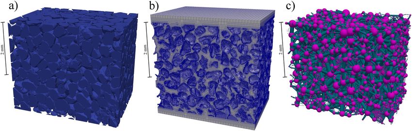
determination of the pressure and velocity fields in the simulated porous media flow. Figure 2 presents an example
of the longitudinal cross-section along the direction of water flow in sample 1d. The uniformly changing pres-
sure can be observed in Fig. 2a and has a pressure gradient enforced by the NS model boundary conditions. The
velocity magnitude field is presented in Fig. 2b, in which areas of higher velocity, caused by the narrow pores,
may be observed.
Saturated conductivity—the dependence on the modeling approach used for estimation. The
NS modeling methodology, unlike PN modeling, accounts for full physical descriptions of the transport phe-
nomena. Additionally, NS modeling relies on true pore space geometry and is presented here as a reference.
Other modeling approaches (e.g., PN and KC) were compared with the NS model. The results of this compari-
son are shown in Fig. 3 together with linear models linking saturated conductivities determined by the PN and
KC methodologies with their NS-based counterparts. Based on these results one can conclude that, compared
to the NS model, the KC-based modeling approach systematically overestimates saturated conductivity values,
as the slope parameter of the linear model (LM) is greater than one (2.169) and the intercept is positive. The
average ratio of KsatKC to K
satNS (KsatKC/NS) is even larger than the slope parameter and is equal to 2.624. On aver-
age, samples analyzed using the KC equation-based estimations are almost three times greater than NS-based
Ksat estimations. The difference between K satNS and KsatKC can also be observed in the subplots of the boxplots
presented in Fig. 3.
The KC equation is known to be only a rough e stimation40 of conductivity, though some discrepancy is not
unexpected. Different studies have shown that KC u nderestimates40,41 or overestimates42 saturated conductivity
depending on the porous medium for which the KC equation is used. In the case of Kuang et al.40, the authors
Scientific Reports | (2021) 11:5859 | https://doi.org/10.1038/s41598-021-85325-z 4
Vol:.(1234567890)www.nature.com/scientificreports/
Figure 2. Simulated water transport through sample 1d shown at a central cross-section of the sample: (a)
kinematic pressure field p [m2 s−2], (b) velocity magnitude field U [m s −1] (figure created using Paraview 5.3
software https://www.paraview.org/).
1.2e−03
Ksat KC
● Ksat PN
8.0e−04
KKC = 2.169 KNS + 5.27e−05
Ksat PN , Ksat KC [ms−1]
●
R2 = 0.987
RMSE = 2.91e−04 ●
1.2e−03
●
●
4.0e−04
6.0e−04
●
●
● ● ●
●
● ●
●
●
●
●
KPN = 1.593 KNS − 7.12e−05 0.0e+00
●
R2 = 0.986
0.0e+00
● ● ●●
● ●
●
●● RMSE = 8.54e−05 Ksat NS Ksat PN Ksat KC
0e+00 1e−04 2e−04 3e−04 4e−04 5e−04
−1
Ksat NS [ms ]
Figure 3. Main plot—saturated conductivities estimated via pore network modeling ( Ksat PN) and Kozeny–
Carman (Ksat KC) modeling compared with the Navier–Stokes (Ksat NS) estimations. The subplot presents boxplots
of the Ksat PN, Ksat KC, and Ksat NS datasets (figure created using RStudio 1.3 software https://rstudio.com/).
used a tortuosity estimation method based on CT porous media images, which generated high tortuosity values
of ~ 4.5 that could lead to conductivity underestimation. Our results, as they relate to the KC saturated conduc-
tivity estimation, are not as overestimated as those reported by Mostaghimi et al.42, in which KC estimation was
also compared with NS estimation. This difference might be due to the different pore space characteristics of
the porous material studied. The greatest overestimation was reported by Mostaghimi et al.42 for samples with
porosities lower than 0.25, which were not observed in the samples used in this study. Taheri et al.43 reported
high levels of agreement between KC and NS saturated conductivity estimations, but their work was related to a
virtual homogeneous sand porous medium built from spherical particles. This medium very closely resembled
the KC equation assumptions. The accuracy of KC estimations may be problematic, but considering how easily
this estimation can be performed in comparison to the application of NS and PN models, the KC method is
suitable in some situations.
Estimations of saturated conductivity via PN modeling are also presented in Fig. 3. In the case of PN estima-
tions, the LM model slope parameter is equal to 1.593, but the intercept is negative. When the average ratio of the
KsatPN to KsatNS (KsatPN/NS) is calculated, it equals 0.927. This result shows that PN-based estimation of the saturated
conductivity gives, on average, practically the same results as NS-based estimations. Boxplots (Fig. 3) confirm
that these two sets (i.e., K satPN and K
satNS) are comparable. This conclusion is also confirmed by a two-sided paired
Scientific Reports | (2021) 11:5859 | https://doi.org/10.1038/s41598-021-85325-z 5
Vol.:(0123456789)www.nature.com/scientificreports/
Figure 4. Relationship between the ratios of saturated conductivities determined by the pore network
(Ksat PN/NS) and Kozeny–Carman (Ksat KC/NS) to saturated conductivities estimated by Navier–Stokes modeling
(figure created using RStudio 1.3 software https://rstudio.com/).
Wilcoxon signed-rank test applied to the saturated conductivity estimation data. In the case of the comparison
between the NS- and PN-based estimations, the result of the test (p-value) is equal to 0.3884, confirming the
hypothesis that the medians of both sets are equal. In the case of the comparison between the NS- and KC-based
estimations, the p-value, 1.9e-6, is far less than the significance level α = 0.05; thus, the medians of these sets are
not equal, which confirms previous statements. Similarly, high levels of agreement between PN and NS estima-
tions were found by Mehmani and T chelepi44 for artificial 2D porous media micromodels. A similar comparison
to the 3D porous media was performed, but for the virtual porous media; Yang et al.26 analyzed one artificial
sphere pack porous medium and found high agreement between PN- and NS-estimated saturated conductivity.
Finally, real 3D porous media were also analyzed by Jiang et al.3 which demonstrated similarly good agreement
when three low resolution (2563 voxels @ 6 µm) rock samples were studied. Our study, which includes larger
and higher-resolution real porous media geometry (~ 14003 voxels @ 2 µm), confirmed the equivalence of NS
and PN estimations.
The relationship of NS-determined saturated conductivity to its PN and KC counterparts, expressed by the
average of the aforementioned ratios (i.e. K satKC/NS and K satPN/NS), does not completely describe the situation.
Regression analysis demonstrates the dependence of both properties, KsatKC/NS (r = 0.72) and KsatPN/NS (r = -0.86),
on the sample’s specific surface, determined based on thresholded images—the same images which were used
for the PN network and NS mesh generation. This dependence is presented in Fig. 4, where K satKC/NS falls within
the range of 2.2–3.5 and KsatPN/NS is in the range of 0.4–1.5.
It is important to note that if K
satKC/NS increases, but K satPN/NS decreases with the increase of the specific surface
σ [m-1]. This means that these opposite trends in the ratios are not caused by the dependence between K satNS
and σ, as if that were the case, the trends would follow a similar pattern. To ensure the possible influence of the
KsatNS estimation error on the values of K satKC/NS and KsatPN/NS, their errors (presented as error-bars in Fig. 4)
were calculated based on error propagation theory. Since the increasing specific surface is related to the particle
size distribution of the material from which the samples were prepared, which in turn influences pore space
complexity, we hypothesized that the observed trend of KsatKC/NS might be connected to the changing tortuosity
of the pore space.
To validate this hypothesis, the tortuosities of the samples were estimated (see Table 1) based on the stream-
lines analysis. The lowest values of tortuosity for the bed of spherical grains, close to the theoretical value of
1.414, were estimated for samples 1u and 1d, which were made of the coarser fraction of sieved sand grains.
However, the majority of samples were made of the milled sand, which consisted mostly of non-spherical grains
where one might expect higher tortuosity to occur. As a result, tortuosity is positively correlated (r = 0.71) with
the image specific surface and the highest values of tortuosity ~ 1.6–1.7 were achieved in samples with a higher
fraction of finely-milled sand.
When these tortuosity estimations were used in the KC Eq. (4) instead of the constant value 1.414, the KC
estimations no longer depended on the value of σ (see data series K satKC/NS (tc) in Fig. 4). This confirms the hypoth-
esis about tortuosity dependence on the pore space complexity.
The results obtained from numerical estimations and from Kozeny-Carman approach were also subjected to
experimental verification (Fig. 5). As per one specimen, for which Ksat was measured, two samples belongs simu-
lated and measured values could not be compared directly. Saturated conductivities estimated for the samples
were recalculated to the specimen’s values according to Eq. (2). In case of NS estimations, error using proposed
Scientific Reports | (2021) 11:5859 | https://doi.org/10.1038/s41598-021-85325-z 6
Vol:.(1234567890)www.nature.com/scientificreports/
Figure 5. Comparison between measured and simulated water conductivities ( KsatEXP—experimentally
determined values for specimens, KsatSIM—values determined based on: NS, PN, and KC estimations; figure
created using RStudio 1.3 software https://rstudio.com/).
approach (Eq. 11) was also for all samples determined. On the figure (Fig. 5) for all specimens KsatNS errors are
presented—they were recalculated based on error propagation theory from appropriate samples’ error estimates.
Conclusions
The PN-estimated saturated conductivity ( KsatPN) was found to be statistically equivalent to NS-determined
saturated conductivity values ( KsatNS). The average value of the K
satPN/KsatNS ratio was equal to 0.927.
The KC equation-based estimation ( KsatKC) overestimated saturated conductivity by more than double (2.624)
the KsatNS estimate. However, despite high levels of overestimation, both sets of values are well-correlated with
R2 = 0.99.
The total porosities of the generated PN were the same as the total porosities of images used for their crea-
tion. Total porosities of numerical meshes were on average lower by 0.01 [m3 m−3] than the porosities of the
corresponding reference images.
Proposed error estimation approach was used for relative error determination of the NS saturated conduc-
tivity modelling. The error was on the average 10% for analyzed samples. The minimum value of the error was
4.6% and maximum 19%. The relative error seem to be higher for fine grained samples. The lowest values of the
relative error was achieved for samples prepared from coarsest sand material.
The tortuosity of 20 samples was estimated. The value of the tortuosity determined for the samples prepared
from coarser fractions of sand approximated the theoretical tortuosity value of the porous medium built from
spherical grains, 1.4. The tortuosities of samples prepared from milled sand (non-spherical grain material) were
higher. The value of tortuosity was correlated (r = 0.71) with the porous medium-specific surface, reaching the
highest values of 1.6–1.7 for samples prepared from the finest sand material.
Materials and methods
Specimens preparation. Specimens were prepared by mixing different unimpaired sieved and milled
sand fractions. The first step in specimen preparation was to sieve the sand using a 0.5 mm sieve. This raw sand
was then milled in the planetary mill (Pulverisette 6 classic line, Fritsch, Germany, Idar-Oberstein). The raw
sand was milled for 5, 10, and 20 min to achieve milled sand fractions with different particle size distributions.
10 specimens were then prepared from a mixture of sieved sand and milled sand fractions. Specimens s1, s2,
and s3 were prepared by sieving raw sand through 0.32, 0.16, and 0.08 mm sieves, respectively. Table 2 presents
the mixing scheme used to create material with diverse particle size distributions (PSD) for the other specimens.
Each prepared specimen’s material prior to the specimen preparation was measured using a laser diffractometry
method (LDM) to verify the PSD that was achieved (Fig. 6). A Malvern Mastersizer 2000 with a measurement
range of 0.02 µm to 2 mm was used for PSD determination. To obtain homogeneity in the sand suspension, a
Hydro G dispersion unit was used, with a pump speed of 1750 rpm and stirrer speed of 700 rpm. Light intensity,
measured with the detectors, was recalculated into PSD according to the Mie theory (ISO 13,320:2009, 2009).
The Mie model parameters include an absorption coefficient of 0.1 and a refractive coefficient of 1.5245. Due to
this specimen preparation procedure, it was possible to evaluate the potential impact of the pore space geometry
on saturated conductivity modeling.
Scientific Reports | (2021) 11:5859 | https://doi.org/10.1038/s41598-021-85325-z 7
Vol.:(0123456789)www.nature.com/scientificreports/
Figure 6. Particle size distribution of sand material used for specimen preparation (figure created using
RStudio 1.3 software https://rstudio.com/).
Figure 7. The geometry of the specimen (ROI up—the region representing upper sample, ROI down—region
representing lower sample; Figure created using Salome 9.6 software https://www.salome-platform.org/).
Scientific Reports | (2021) 11:5859 | https://doi.org/10.1038/s41598-021-85325-z 8
Vol:.(1234567890)www.nature.com/scientificreports/
The specimen was prepared in a polypropylene tube (4 mm internal diameter) of low X-ray absorbance
(Fig. 7). An adequate amount of the specimen’s material was poured into the cylinder to achieve a 10 mm stack
inside the container. The specimen was subsequently compacted in the pipe by vibration. At the bottom and
top of the specimen’s material stack bronze meshes were placed to keep the material in place. In the case of the
specimens (s4, s5, s6, s7, s8, s9, and s10) additionally, the circle cut from filter paper was placed between the mesh
and the material to avoid loss of the fine particles from the specimen. Bronze meshes were used as they were stiff
enough to support properly the specimen’s material, but there was a drawback of this choice. As the metal is far
less penetrated by X-rays than sand, strong streaking artifacts are observed in the reconstructed scans near the
mesh. As a result, the pore space in the neighborhood of the bronze meshes can’t be observed. That was also a
reason for the preparation of relatively high (10 mm) specimens as we would like to ensure a big enough part of
the specimen could be CT analyzed to ensure the reasonable comparison between modeling and measurement of
the saturated conductivity. As the height of the area which is examined using CT is roughly equal to its diameter,
in the 4 mm wide and 10 mm high specimen two samples area were defined.
X‑ray CT sample analysis. An X-ray CT scanner (GE Nanotom 180S) was used to examine the specimens
with a 180 kV/15 W microfocus X-ray tube. For each specimen, two scans were made, one in the upper part of
the specimen and the second in the lower part (Fig. 7). Two regions from each specimen were scanned to achieve
the highest possible CT resolution, which limited the dimensions of the scanned object. This also increased the
number of analyzed samples. As a result, 20 scans were made. They will be referred to as “10d” and “10u,” for
example, where “10d” identifies the lower (downward) part of the 10th specimen and “10u” is the upper part of
the 10th specimen.
For each scan, a series of 1200 2D radiograms were collected, with the specimen rotating through the full
angular range using a rotation step of 0.3°. Each 2D radiogram was averaged over 15 images to reduce noise. The
images were recorded using a detector with a resolution of 2284 × 2304 pixels registering images at the 14-bit
gray-level depth. The X-ray source operated at 90 kV with a 120 μA cathode current and tungsten exit window.
Immediately before each scan, a short pre-scan was performed, which lasted for 30 min to preheat the speci-
men and minimize the impact of thermal expansion during the primary scan for three-dimensional (3D) image
reconstruction. The voxel size achieved in these CT scans was 2 µm.
3D image reconstruction and processing. Tomographic reconstruction was performed using a series
of radiograms (DatosX version 2.0.1, General Electric). The beam hardening correction was not necessary,
although the exit window filter was not used during the X-ray scan. From the obtained 3D volume representing
the sample and a part of the tube, a cubic region of interest (ROI) of 1400 × 1400 × 1700 voxels was chosen for
further processing. Cross-sections of the ROIs of selected samples are presented on the Fig. 8. A median filter
with a three-pixel kernel diameter was applied to the ROI. The next step was thresholding using an IsoData
thresholding method46. Image processing was conducted with Fiji and VGStudio MAX 2.1 (Volume Graphics).
The thresholded images serve as a common starting point for both the PN and NS modeling approaches.
Measurement of the specimen’s saturated conductivity. For each of ten prepared specimens, sat-
urated water conductivity was measured. The measurement was based on the static pressure head principle
(Fig. 9). The pressure difference was fixed, and water flux was measured, then saturated conductivity K [m s−1]
was calculated using Darcy’s law:
ρgq�p
K= (1)
�l
where q [m s −1] is fluid flux, Δp is the pressure difference [Pa] along the sample length Δl [m], g is the gravitational
constant [m s −2], and ρ is fluid density [kg m −3].
The pressure difference was adjusted by changing the water level in the water tank. The value of the differ-
ence in the pressure head was read from the water level difference in the two burettes mounted before and after
the specimen. Water flux was measured based on the scale readings on which the container collecting the water
flowing through the specimen was placed.
The idea of the measurement is simple, but due to very low water fluxes—especially for fine-grained speci-
mens—some additional factors had to been taken into account. To avoid the capillary forces’ influence on the
scale reading, the water container located on the scale was initially filled up to the level little higher than the end
of the glass pipe placed in it. Some of the measurements were long enough to force the water weight loss correc-
tion due to water evaporation from the container placed on the scale. The evaporation rate from the container in
the constant air temperature kept in the laboratory was determined upfront. The last factor that needed correction
was the influence of the bronze meshes and paper filter placed at the ends of the specimen’s material. Five empty
(consisting only from meshes and filter paper) specimens were prepared, and dependence between water flux
and pressure head difference was determined for them. Based on averaged results calibrating function linking
flux with pressure head difference was prepared. Then during regular measurements, based on registered water
flux, appropriate pressure head difference was subtracted from the value read from the burettes.
The results of measured specimen’s saturated conductivities were compared with values of samples conductivi-
ties estimated using different methods. There values cannot be compared directly. But taking into account that
two subsequent samples are defined in one specimen (Fig. 7) one may calculate effective water conductivity Keff
of two stacked samples with conductivities K 1 and K2, as a harmonic average:
Scientific Reports | (2021) 11:5859 | https://doi.org/10.1038/s41598-021-85325-z 9
Vol.:(0123456789)www.nature.com/scientificreports/
Figure 8. Cross-sections of the selected ROIs of the samples: (a) S3u, (b) S5u, (c) S7u, and (d) S9u (figure
created using Fiji 1.5 software https://fiji.sc/).
1 1 1
Keff
=
K1
+
K2 (2)
Pore network saturated conductivity modeling. The thresholded 3D images were processed using
the network extraction code after applying a maximal ball algorithm17. The result was a dataset containing
information about the spherical pores and cylindrical throats including dimensions, spatial coordinates, and
connections47. A simplified pore network (Fig. 10c) was then used for permeability calculations based on the
assumption of laminar flow, the Hagen-Poiseuille formula validity for flow in the throats, and mass conservation
for each pore-throat c onnection48. The boundary condition pressure difference was set between the PN input
and output nodes, resulting in fluid flow throughout the network.
Navier–Stokes saturated conductivity modeling. The NS FVM approach is used to model a single-
phase, laminar, steady-state flow of incompressible fluid through a porous medium. The set of equations used for
the model contains the following momentum balance equation:
D −
−
ρ u = −∇ · T
− ∇pd + F (3)
Dt
Scientific Reports | (2021) 11:5859 | https://doi.org/10.1038/s41598-021-85325-z 10
Vol:.(1234567890)www.nature.com/scientificreports/
Figure 9. The schema of the saturated conductivity measurement laboratory setup (figure created using
Inkscape 0.99 software https://inkscape.org/).
Figure 10. Different approaches to pore space representation: (a) triangulated pore space-solid boundary, the
result of XRT scan, (b) numerical mesh spreading pore network, aligned to real pore space geometry, and c)
simplified pore network representation by the pore network model. All three visualizations are based on sample
1d (figure created using Paraview 5.3 software https://www.paraview.org/).
−
where ρ is the local −fluid density [kg m
−3], u is fluid velocity [m s −1], pd is pressure [Pa], T
is the momentum
], and F is the external forces vector [N m−3].
tensor [N m −2
Additionally, a mass balance for the equation was considered:
−
∇· u= 0 (4)
To solve the NS equations, simpleFoam software was used, which is a part of the OpenFOAM CFD toolbox.
The solver implements a semi-implicit method for pressure-linked equations (SIMPLE) algorithm to solve the
momentum balance equation.
Appropriate boundary conditions were established in the simulation. The fluid velocity was fixed to 1 0–5 m
−1
s , and the pressure was fixed to 0 Pa on the input patch and zero gradient Neuman conditions on the output
patch. Input and output patches were equivalent to the top and bottom sides of the sample. No-slip boundary
conditions were applied to the pore walls. The saturated conductivity was calculated from Darcy’s law using the
pressure drop and fluid velocity at the input boundary.
The first step of an NS simulation using FVM is mesh preparation. The surface of the solid fraction was
determined from the thresholded 3D images and approximated using a triangulated surface mesh (Fig. 10a),
which was saved in an STL format. For pore space surface triangulation, Fiji software was used along with an
isosurface module from the BoneJ plugin49. The mesh (Fig. 10b) was then created based on the STL file using
the snappyHexMesh utility (a part of the OpenFOAM toolkit). Next, the generated mesh was checked for highly
skewed cells and other deficiencies. Cells that did not meet quality constraints, in particular those with skewness
greater than four, were removed to avoid impairing the quality or numerical stability of the simulations. A very
small number, not greater than 0.0282% of the total number of cells, had to be removed.
Scientific Reports | (2021) 11:5859 | https://doi.org/10.1038/s41598-021-85325-z 11
Vol.:(0123456789)www.nature.com/scientificreports/
Kozeny–Carman conductivity estimation. In addition to estimation via the physical modeling
approach, the saturated conductivity of porous media can be also estimated using a phenomenologically derived
formula, the KC equation (Eq. 4), which estimates saturated conductivity based on the total porosity and specific
surface area of the porous medium. The equation is written as40:
φ3 ρg
KKC = (5)
Co τ 2 (1 − φ 2 )σ 2 µ
where KKC is saturated conductivity [m/s], Φ is the total porosity [–], σ is the specific surface area (pore space
surface area per sample volume) [m−1], C0 is the Kozeny constant, τ is the tortuosity [–], ρ is the fluid density [kg
m−3], μ is the dynamic viscosity of the fluid [kg m−1·s−1], and g is the gravitational acceleration constant [m s −2].
0 and τ may be used for conductivity estimation. In this study, we used the most commonly
Different values of C
used values, which are valid for equally-sized spherical granular material: C0 = 2.0 and τ = 1.414. Total porosity
and specific area were determined based on the thresholded 3D images of the samples using an image analysis
approach. Total porosity was determined using the voxel counting method. The specific surface was determined
based on the surface area of the triangulated solid-void interface approximation.
Saturated conductivity estimation errors. Saturated conductivity estimation relies on the modeling
of numerical meshes. In principle, numerical meshes that are generated based on images of a porous medium
should match its overall geometric characteristics (e.g., total porosity). Any discrepancies may lead to errors in
the saturated conductivity estimation50. To account for this, some method of saturated conductivity error esti-
mation is needed. Ideally, error estimation should be based solely on numerical modeling methodology, but it is
not possible. As a an error estimation method, following KC equation-based approach can be used, as it relates
total porosity and specific surface to saturated conductivity. Proposed approach assumes correlation between
KNS and KKC. This correlation in case of samples analyzed here was 0.99. And of course validity of Kozeny-
Carman estimation for pore media in question. Correlation between KNS and K KC means that the following
dependence is assumed:
KNS (φ) = AKKC (φ) (6)
where A is some constant and explicitly dependence on mesh porosity φ was noted. Based on error estimation
theory, the error ΔKNS related to porosity underestimation �φ will be calculated using following equation:
∂KNS (φ)
�KNS (φ0 ) = �φ (7)
∂φ φ0
But taking into account Eq. (6) following equation will be derived:
∂KKC (φ)
�KNS (φ0 ) = A �φ (8)
∂φ φ0
Based on Eq. (5), using the dependence of KC saturated conductivity estimation on total porosity, Eq. (8)
become:
φ2 2φ 2 ρg
�KNS (φ0 ) = A
2 2 2
3+
1 − φ 2 µ φ
�φ (9)
Co τ (1 − φ )σ 0
Which, using Eq. (5) again could be rewritten as:
3 − φ2
�KNS (φ0 ) = AK KC (φ0 )
φ 1 − φ2
�φ (10)
φ0
NS error estimation:
which finally, after taking into account Eq. (6), becomes the formula for relative K
2
�KNS 3 − φ
(φ0 ) =
�φ
φ 1 − φ2 (11)
KNS
φ0
The relative and absolute errors estimated based on this formula are presented in Table 1.
Tortuosity estimation. Porous medium tortuosity is one parameter involved in saturated conductivity
estimation using the KC approach. Tortuosity is related to pore space geometry and pore space complexity. It is
also defined as the ratio of the length of a path between two points to the distance between them.
The tortuosity of porous media can be estimated using either direct analysis of possible paths in 3D porous
media images51 or analysis of a simulated velocity field in a pore space. The velocity field analysis approach may
be used to deduce tortuosity based on the averaged velocity magnitude to longitudinal velocity component ratio52
or streamlines length and distance analysis53. The latter approach was used in this work.
For all samples, fluid velocity fields were simulated using an NS modeling approach. Based on the informa-
tion about pore geometry and the velocity field, streamlines were generated. For each sample, 1000 randomly
Scientific Reports | (2021) 11:5859 | https://doi.org/10.1038/s41598-021-85325-z 12
Vol:.(1234567890)www.nature.com/scientificreports/
Figure 11. Schematic of streamlines analysis used for tortuosity estimation. Streamlines generated based on
pore flow velocity field for the sample 1d (figure created using Paraview 5.3 software https://www.paraview.org/).
distributed streamlines were seeded on the input patch, which were then propagated according to the velocity
field (see Fig. 11). Finally, after discarding the parts of the streamlines that lay outside of the porous medium
related mesh (i.e., in the areas next to input and output patches), the tortuosity value of the sample was estimated
as the average of the tortuosities of the streamlines.
Received: 9 November 2020; Accepted: 1 March 2021
References
1. Fatt, I. The network model of porous media. Trans. AIME 207, 144–181 (1956).
2. Al-Kharusi, A. S. & Blunt, M. J. Multiphase flow predictions from carbonate pore space images using extracted network models.
Water Resour. Res. 44, W06S01 (2008).
3. Jiang, Z. et al. Pore network extraction for fractured porous media. Adv. Water Resour. 107, 280–289 (2017).
4. Wang, Y. D., Chung, T., Armstrong, R. T., McClure, J. E. & Mostaghimi, P. Computations of permeability of large rock images by
dual grid domain decomposition. Adv. Water Resour. 126, 1–14 (2019).
5. Aghaei, A. & Piri, M. Direct pore-to-core up-scaling of displacement processes: Dynamic pore network modeling and experimen-
tation. J. Hydrol. 522, 488–509 (2015).
6. Hannaoui, R. et al. Pore-network modeling of trickle bed reactors: Pressure drop analysis. Chem. Eng. J. 262, 334–343 (2015).
7. Rostami, A., Habibagahi, G., Ajdari, M. & Nikooee, E. Pore network investigation on hysteresis phenomena and influence of stress
state on the SWRC. Int. J. Geomech. 15, 04014072 (2015).
8. Köhne, J. M., Schlüter, S. & Vogel, H.-J. Predicting solute transport in structured soil using pore network models. Vadose Zo. J. 10,
1082 (2011).
9. Mehmani, A., Mehmani, Y., Prodanović, M. & Balhoff, M. A forward analysis on the applicability of tracer breakthrough profiles
in revealing the pore structure of tight gas sandstone and carbonate rocks. Water Resour. Res. 51, 4751–4767 (2015).
10. de Vries, E. T., Raoof, A. & van Genuchten, M. T. Multiscale modelling of dual-porosity porous media; a computational pore-scale
study for flow and solute transport. Adv. Water Resour. 105, 82–95 (2017).
11. Raoof, A., Nick, H. M., Wolterbeek, T. K. T. & Spiers, C. J. Pore-scale modeling of reactive transport in wellbore cement under
CO2 storage conditions. Int. J. Greenh. Gas Control 11, S67–S77 (2012).
12. Xiong, Q., Baychev, T. G. & Jivkov, A. P. Review of pore network modelling of porous media: Experimental characterisations,
network constructions and applications to reactive transport. J. Contam. Hydrol. 192, 101–117 (2016).
13. Hu, M.-C. et al. Development of Kriging-approximation simulated annealing optimization algorithm for parameters calibration
of porous media flow model. Stoch. Environ. Res. Risk Assess. 1–12, https://doi.org/10.1007/s00477-018-01646-y (2019).
14. Bryant, S. & Blunt, M. Prediction of relative permeability in simple porous media. Phys. Rev. A 46, 2004–2011 (1992).
15. Al-Raoush, R. I. & Willson, C. S. Extraction of physically realistic pore network properties from three-dimensional synchrotron
X-ray microtomography images of unconsolidated porous media systems. J. Hydrol. 300, 44–64 (2005).
16. Al-Kharusi, A. S. & Blunt, M. J. Network extraction from sandstone and carbonate pore space images. J. Pet. Sci. Eng. 56, 219–231
(2007).
17. Dong, H. & Blunt, M. Pore-network extraction from micro-computerized-tomography images. Phys. Rev. E 80, 036307 (2009).
18. Nejad Ebrahimi, A., Jamshidi, S., Iglauer, S. & Boozarjomehry, R. B. Genetic algorithm-based pore network extraction from micro-
computed tomography images. Chem. Eng. Sci. 92, 157–166 (2013).
19. Raeini, A. Q., Bijeljic, B. & Blunt, M. J. Generalized network modeling: Network extraction as a coarse-scale discretization of the
void space of porous media. Phys. Rev. E 96, 013312 (2017).
20. Zhao, J., Qin, F., Derome, D., Kang, Q. & Carmeliet, J. Improved pore network models to simulate single-phase flow in porous
media by coupling with lattice Boltzmann method. Adv. Water Resour. 145, 103738 (2020).
21. Khan, Z. A., Elkamel, A. & Gostick, J. T. Efficient extraction of pore networks from massive tomograms via geometric domain
decomposition. Adv. Water Resour. 145, 103734 (2020).
Scientific Reports | (2021) 11:5859 | https://doi.org/10.1038/s41598-021-85325-z 13
Vol.:(0123456789)www.nature.com/scientificreports/
22. Yang, X. et al. Direct numerical simulation of pore-scale flow in a bead pack: Comparison with magnetic resonance imaging
observations. Adv. Water Resour. 54, 228–241 (2013).
23. Moqtaderi, H. & Esfahanian, V. Evaluation of a new solid boundary implementation in the lattice Boltzmann method for porous
media considering permeability and apparent slip. Philos. Trans. R. Soc. A Math. Phys. Eng. Sci. 369, 2193–2201 (2011).
24. Trebotich, D. & Graves, D. An adaptive finite volume method for the incompressible Navier-Stokes equations in complex geom-
etries. Commun. Appl. Math. Comput. Sci. 10, 43–82 (2015).
25. Lesueur, M., Casadiego, M. C., Veveakis, M. & Poulet, T. Modelling fluid-microstructure interaction on elasto-visco-plastic digital
rocks. Geomech. Energy Environ. 12, 1–13 (2017).
26. Yang, X. et al. Intercomparison of 3D pore-scale flow and solute transport simulation methods. Adv. Water Resour. 95, 176–189
(2016).
27. Raeini, A. Q., Bijeljic, B. & Blunt, M. J. Modelling capillary trapping using finite-volume simulation of two-phase flow directly on
micro-CT images. Adv. Water Resour. 83, 102–110 (2015).
28. Raeini, A. Q., Blunt, M. J. & Bijeljic, B. Direct simulations of two-phase flow on micro-CT images of porous media and upscaling
of pore-scale forces. Adv. Water Resour. 74, 116–126 (2014).
29. Verma, R., Icardi, M. & Prodanović, M. Effect of wettability on two-phase quasi-static displacement: Validation of two pore scale
modeling approaches. J. Contam. Hydrol. (article in press) https://doi.org/10.1016/j.jconhyd.2018.01.002 (2018).
30. Ferrari, A., Jimenez-Martinez, J., Borgne, T. L., Méheust, Y. & Lunati, I. Challenges in modeling unstable two-phase flow experi-
ments in porous micromodels. Water Resour. Res. 51, 1381–1400 (2015).
31. Rider, W. J. & Kothe, D. B. Reconstructing volume tracking. J. Comput. Phys. 141, 112–152 (1998).
32. Raeini, A. Q., Blunt, M. J. & Bijeljic, B. Modelling two-phase flow in porous media at the pore scale using the volume-of-fluid
method. J. Comput. Phys. 231, 5653–5668 (2012).
33. Bijeljic, B., Raeini, A., Mostaghimi, P. & Blunt, M. J. Predictions of non-Fickian solute transport in different classes of porous media
using direct simulation on pore-scale images. Phys. Rev. E 87, 013011 (2013).
34. Alhashmi, Z., Blunt, M. J. & Bijeljic, B. Predictions of dynamic changes in reaction rates as a consequence of incomplete mixing
using pore scale reactive transport modeling on images of porous media. J. Contam. Hydrol. 179, 171–181 (2015).
35. Menke, H. P., Bijeljic, B. & Blunt, M. J. Dynamic reservoir-condition microtomography of reactive transport in complex carbonates:
Effect of initial pore structure and initial brine pH. Geochim. Cosmochim. Acta 204, 267–285 (2017).
36. Pereira Nunes, J. P., Blunt, M. J. & Bijeljic, B. Pore-scale simulation of carbonate dissolution in micro-CT images. J. Geophys. Res.
Solid Earth 121, 558–576 (2016).
37. Wu, B., Xu, Y., Zheng, Y. & Fan, J. A new cross-scaling method to deal with the porous flow problem. Theor. Appl. Mech. Lett. 3,
032009 (2013).
38. Liu, M. & Mostaghimi, P. High-resolution pore-scale simulation of dissolution in porous media. Chem. Eng. Sci. 161, 360–369
(2017).
39. Han, Y. & Cundall, P. A. LBM-DEM modeling of fluid - solid interaction in porous media. Int. J. Numer. Anal. Methods Geomech.
37, 1391–1407 (2013).
40. Kuang, X., Sansalone, J., Ying, G. & Ranieri, V. Pore-structure models of hydraulic conductivity for permeable pavement. J. Hydrol.
399, 148–157 (2011).
41. Latief, F. D. E. & Fauzi, U. Kozeny-Carman and empirical formula for the permeability of computer rock models. Int. J. Rock Mech.
Min. Sci. 50, 117–123 (2012).
42. Mostaghimi, P., Blunt, M. J. & Bijeljic, B. Computations of absolute permeability on micro-CT images. Math. Geosci. 45, 103–125
(2013).
43. Taheri, S., Ghomeshi, S. & Kantzas, A. Permeability calculations in unconsolidated homogeneous sands. Powder Technol. 321,
380–389 (2017).
44. Mehmani, Y. & Tchelepi, H. A. Minimum requirements for predictive pore-network modeling of solute transport in micromodels.
Adv. Water Resour. 108, 83–98 (2017).
45. Bieganowski, A., Chojecki, T., Ryżak, M., Sochan, A. & Lamorski, K. Methodological aspects of fractal dimension estimation on
the basis of particle size distribution. Vadose Zo. J. 12, vzj2012.0064 (2013).
46. Ridler, T. W. W. et al. Picture thresholding using an iterative selection method. IEEE Trans. Syst. Man. Cybern. 8, 630–632 (1978).
47. Sochi, T. Non-Newtonian flow in porous media. Polymer (Guildf). 51, 5007–5023 (2010).
48. Valvatne, P. H., Piri, M., Lopez, X. & Blunt, M. J. Predictive pore-scale modeling of single and multiphase flow. Transp. Porous
Media 58, 23–41 (2005).
49. Doube, M. et al. BoneJ: Free and extensible bone image analysis in ImageJ. Bone 47, 1076–1079 (2010).
50. Gackiewicz, B., Lamorski, K. & Sławiński, C. Saturated water conductivity estimation based on X-ray CT images—Evaluation of
the impact of thresholding errors. Int. Agrophys. 33, 49–60 (2019).
51. Sansalone, J., Kuang, X. & Ranieri, V. Permeable pavement as a hydraulic and filtration interface for urban drainage. J. Irrig. Drain.
Eng. 134, 666–674 (2008).
52. Ghassemi, A. & Pak, A. Pore scale study of permeability and tortuosity for flow through particulate media using lattice Boltzmann
method. Int. J. Numer. Anal. Methods Geomech. 35, 886–901 (2011).
53. Duda, A., Koza, Z. & Matyka, M. Hydraulic tortuosity in arbitrary porous media flow. Phys. Rev. E 84, 036319 (2011).
Acknowledgements
This work was partially supported by a grant from the Polish National Centre for Research and Devel-
opment, contract no. PL-TW/IV/5/2017, and the Taiwanese Ministry of Science and Technology:
MOST-106-2923-E−009-001-MY3.
Author contributions
drafting the initial manuscript: B.G., K.L.; modeling and simulation: B.G.; CT experimentation, and measure-
ments: B.G.; study concepts: K.L., C.S.; data analysis: B.G., K.L.; figures: K.L.; project administration: K.L., L-C.C.,
S-Y.H.; manuscript revision and improvements: C.S., S-Y.H., L-C.C.
Competing interests
The authors declare no competing interests.
Additional information
Correspondence and requests for materials should be addressed to K.L.
Reprints and permissions information is available at www.nature.com/reprints.
Scientific Reports | (2021) 11:5859 | https://doi.org/10.1038/s41598-021-85325-z 14
Vol:.(1234567890)You can also read