Ridesharing and Fleet Sizing For On-Demand Multimodal Transit Systems
←
→
Page content transcription
If your browser does not render page correctly, please read the page content below
Ridesharing and Fleet Sizing
                                                                 For On-Demand Multimodal Transit Systems

                                                                             Ramon Auad1,2,? and Pascal Van Hentenryck1,??
                                                       1
                                                            School of Industrial and Systems Engineering, Georgia Institute of Technology, Atlanta, GA
                                                        2
                                                             Departamento de Ingeniería Industrial, Universidad Católica del Norte, Antofagasta, Chile

                                                    Abstract. This paper considers the design of On-Demand Multimodal Transit Systems (ODMTS)
arXiv:2101.10981v1 [math.OC] 26 Jan 2021

                                                    that combine fixed bus/rail routes between transit hubs with on-demand shuttles to serve the first/last
                                                    miles to/from the hubs. The design problem aims at finding a network design for the fixed routes to
                                                    allow a set of riders to travel from their origins to their destinations, while minimizing the sum of the
                                                    travel costs, the bus operating costs, and rider travel times. The paper addresses two gaps in existing
                                                    tools for designing ODMTS. First, it generalizes prior work by including ridesharing in the shuttle
                                                    rides. Second, it proposes novel fleet-sizing algorithms for determining the number of shuttles needed to
                                                    meet the performance metrics of the ODMTS design. Both contributions are based on Mixed-Integer
                                                    Programs (MIP). For the ODMTS design, the MIP reasons about pickup and dropoff routes in order to
                                                    capture ridesharing, grouping riders who travel to/from the same hub. The fleet-sizing optimization
                                                    is modeled as a minimum flow problem with covering constraints. The natural formulation leads to a
                                                    dense graph and computational issues, and is refined in an optimized model working on a sparse graph.
                                                    The methodological contributions are evaluated on a real case study: the public transit system of the
                                                    broader Ann Arbor and Ypsilanti region in Michigan. The results demonstrate the substantial potential
                                                    of ridesharing for ODMTS, as costs are reduced by about 26% with minimal increase in transit times.
                                                    Compared to the existing system, the designed ODMTS also cuts down costs by 35% and reduces transit
                                                    times by 38%.

                                                    Keywords: Ridesharing · Fleet Sizing · Multimodal Transit System · Optimization · On-demand
                                                    Transportation

                                           ?
                                                rauad@gatech.edu, corresponding author
                                           ??
                                                pascal.vanhentenryck@isye.gatech.edu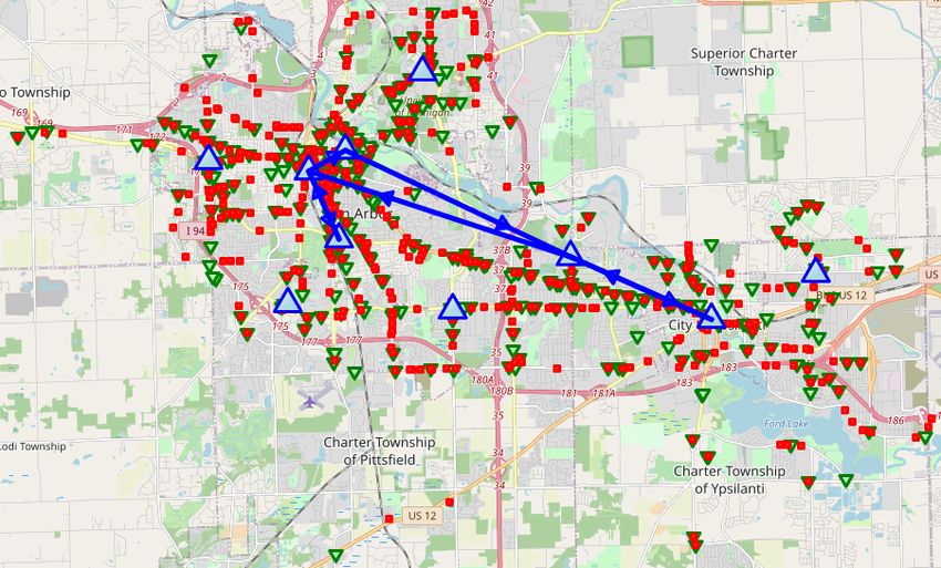
1    Introduction
Recent advances in technology are changing the landscape of city logistics, through the emergence of mobile
applications and the concept of shared mobility (Kulińska and Kulińska, 2019; McCoy et al., 2018). With the
continuous growth in population and urbanization, city logistics is expected to have a significant influence on
a major part of society (Grosse-Ophoff et al., 2017; Raghunathan et al., 2018b; Savelsbergh and Van Woensel,
2016). Consequently, it is crucial to envision novel solutions to meet current challenges in urban logistics,
and develop cost-effective, environmentally friendly, and socially aware (Sampaio et al., 2019) transportation
systems. One promising solution is the integration of shared mobility and multimodal transportation systems,
through a concept known as On-Demand Multimodal Transit Systems (ODMTS) (Van Hentenryck, 2019).
This idea presents significant advantages, including improved mobility for those who do not own a vehicle,
enhanced first and last mile connectivity, expanded access to public transit systems, and a sustainable business
model (Agatz et al., 2020; Kodransky and Lewenstein, 2014; Lazarus et al., 2018; McCoy et al., 2018; Stiglic
et al., 2018) to name a few. This paper explores this concept by integrating ridesharing into the design of an
ODMTS, based on the work by Maheo et al. (2017).
The ODMTS Design Problem has been recently studied by Basciftci and Van Hentenryck (2021); Dalmeijer
and Van Hentenryck (2020); Maheo et al. (2017). ODMTS combine fixed-route bus/rail services between
selected hubs with on-demand shuttles in charge of transporting riders between the hubs and their origins and
destinations. Riders book their trips online (e.g., through a phone app) and are picked up at virtual stops;
this facilitates the passenger pickup and avoids delays due to waiting at a customer residence. Riders are also
dropped off at a location close to their destination. In between, the trip typically involves one or more bus or
rail legs. The tight integration of on-demand shuttle legs with a public transit system may reduce both the
travel time and the overall system cost (Maheo et al., 2017; Stiglic et al., 2018; Van Hentenryck, 2019).
ODMTS also offer the opportunity of grouping, in shared shuttle rides, multiple riders with close origins and
heading towards similar destinations. These ride-shared legs further decrease costs and help in improving
waiting times during peak times. In particular, they offer the possibility of reducing the fleet size for the
shuttles, resulting in lower operational costs and, potentially, increased use of public transport (Farahani
et al., 2013b; Furuhata et al., 2013; Stiglic et al., 2018). However, ridesharing in the shuttle legs and fleet
sizing have not been considered in the original network design optimization of (Maheo et al., 2017) or in
subsequent work.
This paper aims at addressing this gap: it proposes a two-step framework to (1) integrate ridesharing in the
network design optimization and (2) size the shuttle fleet to meet the performance metrics of the proposed
design. More precisely, given a set of origin-destination (O-D) pairs and a set of hubs, this paper addresses
the problem of designing a cost-efficient ODMTS that considers shared shuttle routes and serves all the
transportation requests with the minimum number of shuttles. This relaxes the assumption of Maheo et al.
(2017) that the system always has a shuttle available for serving a request, and provides transit agencies with
a precise estimation of optimal shuttle fleet size, which is critical in practice.
The first step of the framework addresses the ODMTS network design. It selects which pairs of hubs to
connect through high-frequency fixed bus routes in order to take advantage of economies of scale, while
making use of on-demand shuttles for the first and last legs of the trips. There exists a trade-off between the
design of the network and the routing of the passengers via shuttles, since opening a fixed line between hubs
requires a significant investment cost but leads to a low operational cost per trip, whereas shuttle routes
have a low up-front cost but a considerably higher cost per ride. To generate shuttle routes to serve riders,
this paper employs a pickup and dropoff route enumeration algorithm inspired by Hasan et al. (2019). The
constructed routes are then used as input to a Mixed-Integer Program (MIP) that models the ODMTS design
as a Hub-Arc Location Problem (HALP) (Campbell et al., 2005a,b): the model optimally selects the fixed
lines to open and the shuttle routes to serve. The optimal shuttle routes serve as inputs for the second step
of the framework, which addresses the fleet-sizing problem. This second optimization model is a minimum
flow formulation with covering constraints and its coefficient matrix is totally unimodular. It returns the
minimum number of shuttles required to complete all the shuttle requests, and the set of requests served by

                                                       2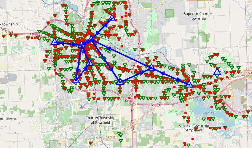
each shuttle. The natural formulation of the fleet-sizing model leads to a dense graph, which raises significant
computational difficulties. An improved formulation, that sparsifies the graph, overcomes these limitations.
The paper presents experimental results to highlight the benefits of incorporating ridesharing into the ODMTS
design in terms of operating cost, passengers convenience, and the number of operating shuttles, using real
data collected from the Ann Arbor Area Transportation Authority (AAATA). The results demonstrate the
substantial potential of ridesharing that improves the ODMTS costs by about 26% while introducing minimal
increases in transit times. Compared to the existing system, the designed ODMTS also cuts down operational
daily costs by 35% and reduces transit times by 38%. The paper also validates the model assumptions by
performing a sensitivity analysis on key ridesharing parameters, including the impact of estimated arrival
times at the last hub and the time window during which riders can be grouped. These results demonstrate
the robustness of the proposed framework.
The contributions of this paper can be summarized as follows:
    (i) it proposes a framework to capture ridesharing in the design of an ODMTS, combining a route-enumeration
        algorithm and a HALP;
 (ii) it presents a totally unimodular flow formulation for determining the optimal fleet size for the on-demand
      shuttles;
(iii) it validates of the proposed framework through a comprehensive set of experiments using real-world
      data from a local public transit system, including a sensitivity analysis of the most critical parameters
      and a comparison with the existing transit system;
(iv) it presents results that demonstrate the substantial benefits of ridesharing for ODMTS and the overall
     benefits in convenience and cost compared to the existing transit system.
The remainder of the paper is organized as follows. Section 2 covers related literature. Section 3 defines the
ODMTS network design problem with ridesharing and the underlying assumptions, provides the mathematical
notation, presents the route enumeration algorithm, and proposes the MIP model for finding the optimal
network design. Section 4 introduces the fleet sizing problem, its assumptions, and its mathematical model.
Section 5 reports the numerical results for the case study in Ann Arbor and Ypsilanti, in Michigan, USA.
Finally, Section 6 presents the concluding remarks and future research directions.

2     Review of Related Literature

In the last several decades, there have been considerable research effort on optimizing the design of urban
transportation networks. A comprehensive review of this line of research is offered by Farahani et al. (2013b),
who compare such problem to the road network design problem (Magnanti and Wong, 1984; Xu et al.,
2016; Yang and H. Bell, 1998) and the public transit network design problem (Bourbonnais et al., 2019;
Cipriani et al., 2012; Demir et al., 2016) in terms of modeling, solution methods, and the most characteristic
constraints. The authors further highlight the effect of computational development, knowledge of solution
methods, and passengers behavior on the evolution of research in design of urban mobility systems. Similar
points are made in the special issue Campbell and Woensel (2019).
The problem studied in this paper concerns urban transportation and has its foundations in the work of
Campbell et al. (2005a,b), which introduce the HALP. They define this problem along with many variants,
where the decision consists of locating a set of arcs between hubs that yields the optimal total flow cost.
Among the presented variants, the HAL4 model has the most similarities with the framework proposed
in this paper as it seeks a connected optimal hub network. However, this paper relaxes some of its key
assumptions: (1) it allows paths that directly connect, through an on-demand shuttle service, an origin with
its corresponding destination; and (ii) it considers solutions with shuttle paths that start or end at a hub
node and visit multiple non-hub nodes.

                                                       3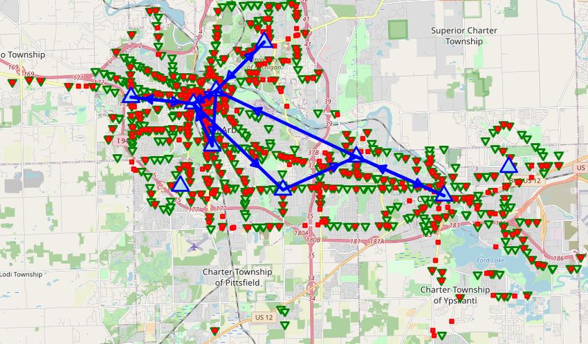
The formulation of the HALP was motivated as an alternative to the hub location problem (HLP) firstly
studied by O’kelly (1986). The HLP is formulated as a binary program, where each decision variable represents
whether a particular node is allocated to a particular hub, and path continuity constraints are imposed. The
HLP, however, assumes that the hubs form a complete network; such critical assumption is relaxed in the
ODMTS design which focuses instead on determining which hub arcs should be opened to obtain economies
of scale. Both problems have a diversity of applications, including the design of large-scale transportation
systems, where there are strong opportunities of cost efficiency through consolidation of passengers (Campbell
and O’Kelly, 2012; Lium et al., 2009). In particular, Campbell and O’Kelly (2012) address the origins and
evolution of the hub location field, and Alumur and Kara (2008); Farahani et al. (2013a) present an exhaustive
survey on hub location literature.
This work is closely related to Dalmeijer and Van Hentenryck (2020); Maheo et al. (2017). Maheo et al.
(2017) introduces the ODMTS design problem as part of the BusPlus project, seeking to improve the public
transportation in the city of Canberra, Australia. By only considering single-passenger shuttle rides, they
formulate the design problem as a MIP and identify a special structure in the formulation suitable to employ
a Benders decomposition algorithm that generates multiple cuts per iteration (Benders, 2005). Moreover,
they speed up its convergence by executing a pre-processing step that detects trips for which direct shuttle
trip are optimal, and further accelerate the solving process through the generation of Pareto-optimal Benders
cuts (Magnanti and Wong, 1981). This work is later extended by (Dalmeijer and Van Hentenryck, 2020) who
incorporate the selection of the frequency of each opened bus leg and constraints on the number of transfers
using a transfer-expanding graph. This allows a Benders decomposition formulation where the sub-problem
solves multiple independent shortest path problems. The authors show the effectiveness of this approach
using real data from the city of Atlanta, GA.
Unfortunately, the incorporation of ridesharing into the problem modeling breaks such structure, and
consequently neither the Benders cut disaggregation nor the aforementioned pre-processing steps are possible
while preserving optimality. If the design optimization is decomposed into a restricted master problem and
a sub-problem as in Maheo et al. (2017), the sub-problem linear relaxation no longer has extreme integer
points, and hence a standard Benders decomposition does not converge to the true optimal solution. Despite
such issue, it is still possible to solve instances of reasonable sizes that consider ridesharing in the shuttle legs
by only limiting shuttle routes to the ones that satisfy reasonable real-world criteria (e.g., timing constraints).
Enforcing these conditions makes it possible to enumerate all the reasonable routes without incurring excessive
running times, even for real cases as the one considered in this paper. The route enumeration algorithm in
this paper is inspired by the approach in Hasan et al. (2019), which studies community-based ridesharing.
Both algorithms enumerate shared shuttle routes to connect to/from a specific location (a job center in Hasan
et al. (2019) and hubs in the present paper). As long as the shuttle capacity is not excessively large and only
routes of practical interest are considered, the algorithm generates all the routes of potential interest in short
times.
Another related line of work include research in last-mile logistics. Raghunathan et al. (2018a) optimizes total
transit time considering the joint schedule of passengers that make use of mass transportation (represented by
a train) and fixed shuttle capacity. In this setting, passengers take the train at a given time from a particular
station to a common origin hub, from where they are consequently grouped in shuttle rides that drop them
at their final destinations. Under specific conditions, they characterize a set of optimal solutions and further
propose a heuristic method that exploits such solution structure. In a later work Raghunathan et al. (2018b),
the authors propose a more general model that optimizes a convex combination of two objectives, namely
total transit time and number of shuttle trips. Combining decision diagrams and branch-and-price, they are
able to solve real-world instances to optimality in very short times. Additionally, a study of a variant of the
work of Raghunathan et al. (2018b) with uncertainty in the schedule of a subset of passengers can be found
in Serra et al. (2019). The key assumptions present in all these papers are (i) a single hub from where shuttle
rides start; (ii) all the stations from where passengers take the initial leg are fixed and visited sequentially;
and (iii) any shuttle route has a unique stop and every customer in the ride is dropped off at this stop. This
paper relaxes some of these assumptions by considering trips with first and last shuttle legs and middle legs

                                                         4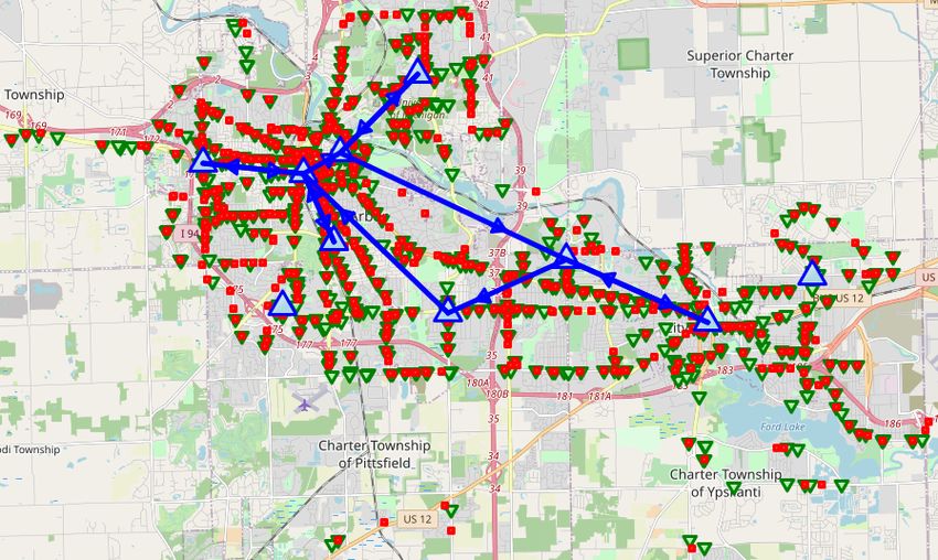
in fixed bus routes, and by making the bus network design a key part of the decision problem. Moreover,
shuttle routes may perform multiple intermediate stops to serve riders with different origins and destinations,
potentially requiring fewer shuttles to serve all the requests.
In relation to fleet size optimization, Raghunathan et al. (2018b); Serra et al. (2019) study a problem that
under some specific parameters is equivalent to minimizing the number of shuttle rides. A survey on fleet
planning is provided in Baykasoğlu et al. (2019), which focuses on single and multi-modal transportation
systems. Contexts where fleet sizing is of particular importance include meal delivery (Auad et al., 2020) and
airline scheduling (Wang et al., 2015).

3      Network Design with Ridesharing

This paper considers the design of an ODMTS that features fixed bus lines, on-demand shuttles to serve the
first and last miles, and the possibility of ride-sharing. The objective function jointly minimizes the total cost
of the system, i.e., the fixed cost of operating the bus lines and the variable cost of each shuttle trip, and
the inconvenience of the passengers, i.e., the transit time from origin to destination. The design makes the
following assumptions.
    • Every shuttle has the same finite capacity.
    • Passengers with a common O-D pair and departure time are grouped into a single commodity3 up to the
      shuttle capacity. If the total number of passengers with common O-D pair and departure time exceeds
      the shuttle capacity, the request is split into multiple commodities.
    • Shuttle routes can be of three types: a direct O-D route, a pickup route, or a dropoff route. A direct route
      serves a trip from its origin to its destination and has no ride sharing. A pickup route starts at a pickup
      location, may involve multiple intermediate stops to pick up riders at different locations, and drops all of
      them off together at a particular hub. A dropoff route starts at a bus hub with a set of passengers on
      board, makes a set of sequential stops to drop each of them off, and ends at the destination of the last
      rider.
    • Shuttle routes may involve multiple passengers, as long as (i) the individual departure times of the
      passengers included in the shared route fall in a common predefined time window; and (ii) the total time
      that each involved passenger spends aboard the shuttle does not exceed a predefined time threshold
      relative to the duration of the direct route.
    • Buses are considered to be available for connections after a fixed waiting time.

3.1     Problem Formulation

The design input contains the following elements:
    (i) a complete graph G with a set N of nodes, where the nodes represent virtual stops and the arcs represent
        links between them;
 (ii) a subset H ⊆ N of nodes that are designated as bus hubs; bus lines are only between hubs;
(iii) time and distance matrices T and D that respect the triangle inequality but can be asymmetric: for
      each i, j ∈ N , Tij and Dij denotes the time and distance from node i to j, respectively;
(iv) a set C of commodities (trips) to serve: each commodity r ∈ C is characterized by an origin or(r), a
     destination de(r), a number of passengers p(r), and a departure time t0 (r);
 (v) A time horizon [Tmin , Tmax ] during which departures occur, i.e., t0 (r) ∈ [Tmin , Tmax ], ∀r ∈ C.
3
    The terms commodity and trip are interchangeably used throughout this work, and refer to a set of passengers with
    a common O-D pair and departure time.

                                                          5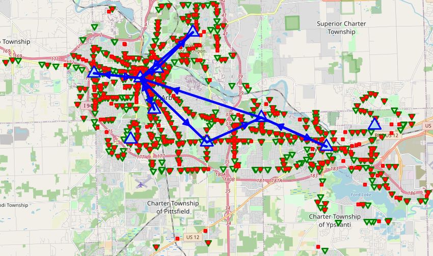
The ODMTS problem jointly optimizes the fixed cost of opening bus lines, a distance-based cost incurred
by the system, and the inconvenience of passengers measured in terms of travel time. The distance cost is
computed by multiplying the travel distance by the corresponding shuttle and bus variable costs. To capture
the sub-objectives in a single cost function, the model uses a conversion factor α that represents a “value of
time”: a rider inconvenience is translated to a cost by multiplying the total travel time (including waiting
times during transfers) by α. The objective function is thus the sum of the total inconvenience and the
operational cost multiplied by (1 − α). Higher values of α give more priority to minimizing inconvenience,
while lower values translate into an optimal solution that primarily seeks to minimize costs. The following
nomenclature is used to compute the total cost:
 • K: shuttle passenger capacity;
 • c: variable cost per kilometer of a shuttle;
 • b: variable cost per kilometer of a bus;
 • n: the number of buses per time period for a given bus line if opened (assumed to be the same for each
   opened bus line);
 • S: the fixed bus waiting time incurred by a passenger at a given bus hub.
The cost function associated with each mode of transportation accurately captures its characteristics. For
               .
buses, let BL = {(h, l) ∈ H × H : h 6= l} be the set of possible bus lines that can be opened. The decision of
opening a bus line requires a cost equivalent to the cost of running n buses during a time period of interest
(thus this cost is modeled as a one-time setup payment). More precisely, for any (h, l) ∈ BL, the cost of
opening a bus line from h to l during a time period of interest is explicitly given by
                                                .
                                           βhl = (1 − α)b · n · Dhl
Once bus line (h, l) is opened, the cost incurred by a passenger from using such line is only the associated
converted inconvenience, i.e.,
                                                  .
                                              γhl = α(Thl + S)

For a commodity r ∈ C, since waiting and travel times are incurred by each passenger, the inconvenience
cost of the p(r) riders using bus line (h, l) ∈ BL is computed as
                                                  r .
                                                 γhl = p(r) · γhl

This definition assumes that buses have infinite capacity (they are almost never full in simulation studies),
which means that the p(r) riders can always follow the same multi-modal route. Each shuttle route ω is
characterized by
 • kω : the number of commodities served by route ω.
 • r ω : a vector of commodities (r1ω , r2ω , . . . , rkωω ) served by a shuttle following route ω, where rjω corresponds
   to the j-th commodity picked up (dropped off) in a pickup (dropoff) shuttle route.
 • hω : the bus hub associated with route ω; in pickup routes, hω corresponds to the route ending point; in
   dropoff routes, hω corresponds to the starting point of the route; direct O-D routes do not involve hubs
   and so this parameter does not apply.
 • ξ ω : a time vector (ξ1ω , ξ2ω , . . . , ξkωω ) where ξjω denotes the total time that commodity rjω incurs to complete
   route ω, i.e., the time from departure time t0 (rjω ) to when rjω leaves the shuttle.
 • pω : the total number of passengers picked up (dropped off) by a shuttle following route ω, with
                                                               kω
                                                         . X
                                                      pω =   p(rjω )
                                                            j=1

                                                           6
• Aω : the set of arcs (i, j) ∈ N × N traversed by a shuttle following route ω.
• dω : the total distance driven by a shuttle following route ω, i.e.,
. X
dω = Dij
(i,j)∈Aω
• cω : the total cost (combining distance cost and inconvenience) incurred by a shuttle following route ω,
computed as
kω
. X
cω = (1 − α)c · dω + α p(rjω ) · ξjω
j=1
Direct shuttle routes result in a lower inconvenience, but routes serving multiple trips have lower costs. To
illustrate this trade-off, consider a small instance with commodities C = {r1 , r2 } with p(r1 ) = p(r2 ) = 1 and
t0 (r1 ) = t0 (r2 ) = 0, and a hub h. Furthermore, assume Tor(r),h = 5, Dor(r),h = 4, ∀r ∈ C, Tor(r1 ),or(r2 ) = 2,
and Dor(r1 ),or(r2 ) = 1. If each commodity r ∈ C takes a direct shuttle route ωr from or(r) to h, then the total
shuttle cost is given by
cω1 + cω2 = (1 − α)c · (dω1 + dω2 ) + α(p(r1 ) · ξ1ω1 + p(r2 ) · ξ1ω2 )
= (1 − α)c · (Dor(r1 ),h + Dor(r2 ),h ) + α(1 · Tor(r1 ),h + 1 · Tor(r2 ),h )
= (1 − α)c · (4 + 4) + α(5 + 5)
= 8c(1 − α) + 10α.
Alternatively, consider a shared route ω1,2 that sequentially picks up commodities r1 and r2 , and then drops
them off at hub h, i.e., Aω1,2 = {(or(r1 ), or(r2 )), (or(r2 ), h)}. In this case, the total shuttle cost corresponds
to
ω ω
cω1,2 = (1 − α)c · dω1,2 + α(p(r1 ) · ξ1 1,2 + p(r2 ) · ξ2 1,2 )
= (1 − α)c · (Dor(r1 ),or(r2 ) + Dor(r2 ),h )
+ α · 1 · (Tor(r1 ),or(r2 ) + max{0, t0 (r2 ) − t0 (r1 ) − Tor(r1 ),or(r2 ) } + Tor(r2 ),h )
+ α · 1 · (max{0, t0 (r1 ) + Tor(r1 ),or(r2 ) − t0 (r2 )} + Tor(r2 ),h )
= (1 − α)c · (1 + 4) + α(2 + max{0, −2} + 5) + α(max{0, 2} + 5)
= 5c(1 − α) + 14α.
The cost savings of employing ridesharing are cω1 + cω2 − cω1,2 = 3c(1 − α) − 4α. It follows that distance cost
savings (3c(1 − α) in the example) may exist when the distance between pickup locations is small compared
to the sum of individual distances from pickup locations to hub h, and they may outweigh the increase in
inconvenience cost (in the example, 4α).
3.2 The MIP Model
This section presents the MIP model associated with the design of the ODMTS. The MIP model receives as
input a set of shuttle routes and uses the following notations:
• Ωr− : the set of pickup routes ω such that r ∈ r ω for commodity r ∈ C;
• Ωr+ : the set of dropoff routes ω such that r ∈ r ω for commodity r ∈ C.
. S . S
The set of pickup routes is denoted by Ω − = r∈C Ωr− and the set of dropoff routes by Ω + = r∈C Ωr+ . The
construction of these routes is discussed in Section 3.3.
7X X X X X
min βh,l zh,l + τr ηr + cp xp + cp xp + r
γh,l r
yh,l (1a)
(h,l)∈BL r∈C p∈Ωr− p∈Ωr+ (h,l)∈BL
X X
s.t. zh,l = zl,h ∀h ∈ H (1b)
l∈H l∈H
X
ηr + xp ≥ 1 ∀r ∈ C (1c)
p∈Ωr−
X
ηr + xp ≥ 1 ∀r ∈ C (1d)
p∈Ωr+
r
yh,l ≤ zh,l ∀(h, l) ∈ BL, ∀r ∈ C (1e)
X X X X
r
yl,h + xp = r
yh,l + xp ∀r ∈ C, ∀h ∈ H (1f)
l∈H p∈Ωr− l∈H p∈Ωr+
if ph =h if ph =h
r
zh,l , yh,l , xp , ηr ∈ {0, 1} (1g)
Fig. 1: The MIP Model for the ODMTS with Ridesharing.
The MIP model considers two interacting decisions: it determines (i) which bus lines to open, and (ii) which
route riders follow from their origin to their destination, either using a direct route or multi-modal routes
combining shuttle and bus legs. Multi-modal routes can only use opened bus legs. The MIP formulation
models these decisions using the following binary decision variables: zh,l = 1 iff bus line (h, l) ∈ BL is selected
to be opened; yh,l
r
= 1 iff riders in r ∈ C take bus line (h, l) ∈ BL; xω = 1 iff shuttle route ω ∈ Ω − ∪ Ω + is
selected to be served; ηr = 1 iff riders in r ∈ C take a direct shuttle route from or(r) to de(r).
Figure 1 presents the MIP model that optimally designs the ODMTS. Objective (1a) minimizes the total
cost, which includes the routing costs (the cost and inconvenience of direct and multi-modal routes) and
the cost of opening bus lines. Constraints (1b) enforce a weak connectivity on the resulting bus network,
requiring that, for each hub h ∈ H, the number of opened bus lines inbound to h must match the number of
outbound opened lines. As mentioned in Maheo et al. (2017), although (1b) by itself does not theoretically
guarantee full connectivity of the resulting bus network, in practice, the spatial distribution of the origins and
destinations makes this set of constraints sufficient for this purpose. Constraint sets (1c) and (1d) guarantee
that each commodity r ∈ C is both picked up at its origin and dropped off at its destination, either by a
direct or a shared route. Constraints (1e) restrict bus legs to only use opened bus lines, and Constraints (1f)
enforce the flow conservation constraints at each hub.
3.3 The Route Enumeration Algorithm
This section describes the generation of the shared routes used as inputs for the MIP model in Figure 1.
Practical Considerations The algorithm restricts attention to routes of practical interest, using a route
duration threshold δ > 0 and a consolidation time window length W > 0. Consider a sequence of m ≥ 1
commodities (r1 , r2 , . . . , rm ) and a hub h ∈ H. In order for the route enumeration algorithm to define a route
ω with r ω = (r1 , r2 , . . . , rm ) and hω = h, ω must satisfy three conditions:
1. if ω is a pickup route, ξjω ≤ (1 + δ) · Tor(rjω ),h , j ∈ {1, 2, . . . , m};
2. if ω is a dropoff route, ξjω ≤ (1 + δ) · Th,de(rjω ) , j ∈ {1, 2, . . . , m};
3. pω ≤ K.
8Algorithm 1 Pickup Route Enumeration
Input: C, K, H, δ
Output: For each r ∈ C, set of pickup routes Ωr−
1: for r1 ∈ C do
2: Ωr−1 ← ∅
3: for h ∈ H do
4: Ωr−1 ← Ωr−1 ∪ {or(r1 ) → h}
5: for k ∈ {2, . . . , K} do
6: σperm ← {All (k − 1)-element permutations of trips (r2 , . . . , rk ) ∈ (C \ {r1 })k such that a route
ω with r = (r1 , r2 , . . . , rk ) and hω = h satisfies practical conditions 1, 3 and 4}
ω
7: for (r2 , . . . , rk ) ∈ σperm do
8: ω ← pickup route with r ω = (r1 , r2 , . . . , rk ) and hω = h
9: for j ∈ {1, 2, . . . , k} do
10: Ωr−j ← Ωr−j ∪ {ω}
Condition 1 requires that the total time spent by commodity rj in a shared pickup route towards hub h does
not exceed (1 + δ) times the duration of the direct shuttle route from or(rj ) to h, and condition 2 imposes
similar requirements for dropoff routes. Condition 3 enforces that the number of riders served by a route
cannot exceed the shuttle capacity K.
Ride-shared routes should only consider riders with close departure times. The operating time horizon
[Tmin , Tmax ] is partitioned into d TmaxW −Tmin
e time windows of W minutes. A set of commodities can be served
by a shuttle route only if their departure times lie in one of these W -minute time windows. Pickup routes
can easily be consolidated based on the departure times of their riders (i.e., t0 (r), r ∈ C). However, dropoff
routes raise an interesting issue since the arrival of riders at their starting hubs requires an ODMTS design.
To overcome this difficulty, for each commodity r ∈ C and each hub l, the algorithm approximates the
time t1 (r, l) when the p(r) riders may reach hub l in their path toward their final destination de(r); this
approximation is then used to decide which commodities can be grouped together in a dropoff route. This
estimation is computed as the average of the total travel times obtained from each of the |H| paths that start
at or(r) at time t0 (r), travel by shuttle to one of the |H| existing hubs, and then take a bus leg to l, i.e.,
. 1
X
t1 (r, l) = t0 (r) + |H| (Tor(r),h + S + Th,l ).
h∈H
Note that the only purpose of this approximation is to decide which riders may be grouped together to avoid
the generation of impractical shared routes. As a result, a shuttle route ω shared by any two commodities
r, s ∈ C must satisfy one of the following timing conditions:
4. if ω is a pickup route, then there exists q ∈ Z+ such that t0 (r), t0 (s) ∈ [Tmin + qW, min{Tmin + (q +
1)W, Tmax }];
5. if ω is a dropoff route, then there exists q ∈ Z+ such that t1 (r, hω ), t1 (s, hω ) ∈ [Tmin + qW, min{Tmin +
(q + 1)W, Tmax }].
These considerations are motivated by the fact that riders may not agree to share a shuttle if the shared
route results in considerably longer travel or waiting times.
The Algorithm This section describes the algorithm to construct the sets of routes Ωr− and Ωr+ for every
commodity r ∈ C, considering homogeneous shuttles with fixed capacity K. Algorithm 1 shows a general
sketch of the enumeration process for Ωr− . For each r1 ∈ C and hub h ∈ H, the algorithm first generates the
individual pickup route that travels from or(r1 ) to h (lines 3 - 4). Then for the multi-passenger routes, it sets
commodity r1 as the first pickup in the route and iterates over all the possible permutations of sizes 1 up to
9K − 1 of the remaining commodities in C, considering only permutations of commodities whose travel time
in ω satisfies Conditions 1, 3, and 4 (5 - 6). For each of such permutations, the algorithm constructs a route
ω that picks up commodities r1 , r2 , . . . , rk in that order and drops them off at hub h (line 8) and adds this
route to the set of pickup routes Ωr−j of each picked up commodity rj , j ∈ {1, . . . , k} (line 10). The procedure
is repeated by fixing every commodity r ∈ C to be the first pickup in a route. The algorithm to construct
the set of dropoff routes Ωr+ follows an almost identical sequence of steps as Algorithm 1. To speed up the
enumerating process, the algorithms are implemented using a depth-first approach that prunes the search
space using the number of passengers and the duration of the constructed route. In addition, although these
algorithms may generate multiple routes that serve a same subset of commodities C in different order, only
the least cost route among them is of practical interest, since the optimization model always selects the least
cost route over the other routes covering the same commodity subset C. This allows to significantly reduce
the number of routes generated by this enumerating process.
4 Fleet-Sizing Optimization
This section discusses the fleet-sizing optimization that minimizes the number of shuttles needed by the
ODMTS. It starts with a general formulation which is then improved for computational efficiency.
4.1 General Formulation
Given the set of optimal routes defined by solution vectors η ∗ , x∗ , and y ∗ from solving the ODMTS design
model in Figure 1, this section presents a MIP model which minimizes the number of shuttles required to
serve all the shuttle routes on time. Recall that the route enumeration algorithm uses an estimate t1 (r, l) for
the arrival at hub l of commodity r. After solving the ODMTS design model, this estimate can be replaced
by its actual arrival time t̃1 (r, hω ) in the designed network, computed as
. X
t̃1 (r, hω ) = t0 (r) + ξ1p x∗ω + r∗
(Th,l + S)yh,l
(h,l)∈BL
when ηr∗ = 0 and x∗ω = 1.
The input for the fleet-sizing optimization is a set of shuttle routes Ω obtained by solving the ODMTS design
model, where each route ω ∈ Ω is characterized by a start location `ω 0 , an end location `f , a start time τω ,
ω
and a duration ∆ω . In particular,
• If ω is a pickup route, then (`ω
0 , `f , τω , ∆ω ) = (or(r1 ), hω , t0 (r1 ), ξ1 ). The route starts at location or(r1 )
ω ω ω ω ω
where the first commodity r1 is picked up at departure time t0 (r1 ). Moreover, the route ends at the hub
ω ω
hω , where all the pickups are dropped off for a total duration of ξ1ω .
• If ω is a dropoff route then (`ω
0 , `f , τω , ∆ω ) = (hω , de(rkω ), maxj {t̃1 (rj , hω )}, ξkω ). The route starts at
ω ω ω ω
hub hω when all commodities r arrive to hω and the start time is computed as maxj {t̃1 (rjω , hω )}. The
ω
route ends at de(rkωω ) when the last commodity rkωω is dropped off and hence its duration is ξkωω .
• Direct O-D routes are also considered in the set of routes Ω. Particularly, for each r ∈ C such that ηr∗ = 1,
Ω considers p(r) additional individual routes, each with (`ω ω
0 , `f , τω , ∆ω ) = (or(r), de(r), t0 (r), Tor(r),de(r) ).
Each of these routes starts at location or(r) at t0 (r) and travels directly to de(r), arriving at time
t0 (r) + Tor(r),de(r) .
The fleet-sizing optimization first builds a directed graph G = (V, A) with a unique source node s and
sink node s0 , and where each node in V \ {s, s0 } uniquely represents a shuttle route in Ω. As a result, the
presentation in this section uses “node” and “route”, as well as V \ {s, s0 } and Ω, interchangeably. The source
connects to every node ω ∈ Ω through an arc (s, ω), and every node ω ∈ Ω connects to the sink s0 via an
10Algorithm 2 The Fleet-Sizing Graph Construction.
Input: Set of routes Ω.
Output: Task network G = (V, A).
1: Let s and s0 be the source and sink nodes, respectively.
2: V ← Ω ∪ {s, s0 }, A ← ∅
3: for ω ∈ Ω do
4: A ← A ∪ {(s, ω), (ω, s0 )}
5: for µ ∈ {ω 0 ∈ Ω : τω0 > τω } do
6: if τω + ∆ω + T`ωf ,`µ0 ≤ τµ then
7: A ← A ∪ {(ω, µ)}
X
min vs,ω (2a)
ω∈δs+
X
s.t. vµ,ω = 1, ∀ω ∈ Ω (2b)
−
µ∈δω
X X
vµ,ω = vω,µ , ∀ω ∈ Ω (2c)
− +
µ∈δω µ∈δω
vω,µ ∈ {0, 1}, ∀(ω, µ) ∈ A (2d)
Fig. 2: The MIP model for Fleet-Size Minimization.
arc (ω, s0 ). Furthermore, for each pair of routes ω, µ ∈ V \ {s, s0 }, there is an arc (ω, µ) ∈ A when a single
shuttle may feasibly serve routes ω and µ in that order, i.e., when τω + ∆ω + T`ωf ,`µ0 ≤ τµ . The construction
algorithm for G is shown in Algorithm 2.
The fleet-sizing optimization uses a binary decision variable vω,µ for each route pair (ω, µ) ∈ A whose value
.
is 1 iff a shuttle serves route µ immediately after serving route ω. Let δω− = {ω 0 ∈ V : (ω 0 , ω) ∈ A}, and
+ .
δω = {ω ∈ V : (ω, ω ) ∈ A}. Figure 2 presents the MIP model to minimize the fleet size needed to serve
0 0
all the selected shuttle routes associated with a given hub. Objective (2a) captures the number of shuttles
needed to cover all routes as the total flow from the source s to any other node. Constraints (2b) require that
every route ω ∈ Ω is visited by one unit of flow, and Constraints (2c) enforce flow conservation at all nodes
other than the source and sink. The coefficient matrix of the fleet-sizing model is totally unimodular: since
the right-hand side is integer, the model can be formulated as a linear program.
Figure 3 provides an example of the output of Algorithm 2 for a simple instance with Ω = {1, 2, . . . , 6}.
Routes are indexed based on the start time, with smaller index implying earlier start time.4 Given that the
arcs represent all the feasible sequential completion of routes, at least 3 shuttles are required to complete
all the requests on time. The solution of this formulation also specifies the sequence of routes each shuttle
serves, which opens the possibility to optimize other objectives that depend on this information (e.g., driven
distance, total travel time).
4.2 A Sparse Fleet-Sizing Formulation
Experimental results on solving the fleet-sizing model in Figure 2 indicated that practical case studies create
an excessive number of feasible arcs, slowing down the solving process considerably due to the large number
4
Note that arc (2, 4) is not defined even though (2, 3) is and τ3 < τ4 . This is because the repositioning time T`2 ,`4 is
f 0
too long for a single shuttle to serve routes 2 and 4 in sequence.
11Fig. 3: A Fleet-Sizing Graph with |Ω| = 6 Routes and an Optimal Fleet Size of 3.
Algorithm 3 The Sparse Fleet-Sizing Graph Construction.
Input: List of routes Ω sorted by earliest start route.
Output: Task network G = (V, A).
1: Let s and s0 be source and sink nodes, respectively.
2: V ← Ω ∪ {s, s0 }, A ← ∅
3: for ω ∈ Ω do
4: for µ ∈ Ωω do
5: if {ω 0 ∈ Ωω : µ ∈ Ωω0 } = ∅ then
6: A ← A ∪ {(ω, µ)}
−
7: if δω = ∅ then
8: A ← A ∪ {(s, ω)}
9: for ω ∈ Ω do
10: if δω+ = ∅ then
11: A ← A ∪ {(ω, s0 )}
of variables and significant memory consumption. To overcome these computational issues, this section
introduces an arc filtering procedure that results in a significantly sparser fleet-sizing graph. The key idea
underlying the filtering is rooted in the fact that shuttles are formulated as a flow and that computing the
optimal fleet size only requires ensuring that every node is visited by at least one shuttle; as long as this is
satisfied, it is not necessary to explicitly define all the arcs between routes. As a result, it is possible to reduce
the number of arcs by removing transitive arcs between routes: if arcs (ω1 , ω2 ) and (ω2 , ω3 ) are defined, then
it is not necessary to define arc (ω1 , ω3 ) even though it represents a feasible service sequence. Instead, it is
sufficient to remove the capacity limit of arcs (ω1 , ω2 ) and (ω2 , ω3 ) and to allow “multiple shuttles” to traverse
the arcs. Once the new formulation is solved, it is possible to recover the path followed by each shuttle. At
termination, the algorithm produces a set of routes whose cardinality matches to the optimal fleet size.
12X
min vs,ω (3a)
ω∈δs+
X
s.t. vµ,ω ≥ 1, ∀ω ∈ Ω (3b)
−
µ∈δω
X X
vµ,ω = vω,µ , ∀ω ∈ Ω (3c)
− +
µ∈δω µ∈δω
vω,µ ∈ Z+ , ∀(ω, µ) ∈ A (3d)
Fig. 4: The Sparse MIP Model for the Fleet-Sizing Optimization.
Algorithm 4 Recovery of Shuttle Paths
Input: Optimal flow vector v ∗ from the sparse fleet-sizing model.
Output: Set of shuttle paths P .
1: P ← ∅
2: Ω ← Ω
3: while v ∗ 6= 0 do
4: p←∅
5: Identify a path Apath = {(s, ω1 ), (ω1 , ω2 ), . . . , (ωk , s0 )} such that va∗ > 0, ∀a ∈ Apath .
6: for a ∈ Apath do
7: va∗ ← va∗ − 1
8: for j ∈ {1, 2, . . . , k} do
9: if ωj ∈ Ω then
10: p ← p ∪ {ωj }
11: Ω ← Ω \ {ωj }
12: P ← P ∪ {p}
.
To formulate the new graph construction algorithm, consider each route w ∈ Ω and let Ωω = {w0 ∈ Ω :
τω + ∆ω + T`ω ,`ω0 ≤ τω0 } be the set of routes that may be served immediately after ω with the same shuttle.
f 0
The modified network construction procedure is then presented in Algorithm 3. For routes ω ∈ Ω and µ ∈ Ωω ,
the arc (ω, µ) is created only if no intermediate route ω 0 exists such that ω 0 ∈ Ωω and µ ∈ Ωω0 , as stated in
lines 5 and 6.
Given this new fleet-sizing graph, it is possible to define a new optimization model with the following
decision variables: variable vω,µ represents the number of shuttles traversing arc (ω, µ). The sparse fleet-sizing
optimization model is shown in Figure 4. Objective (3a) minimizes the total number of shuttles used to
complete all the routes. Constraints (3b) ensure that every node is visited by at least one shuttle; this is
a relaxation with respect to model in Figure 2 that is necessary due to the more limited number of arcs
in the sparser graph. Constraints (3c) enforce flow conservation at all nodes, and Constraints (3d) admit
uncapacitated flows but requires them to take integer values. Given an optimal flow vector v ∗ , it is possible
to recover the paths followed by each shuttle by executing Algorithm 4.
The sparse graph construction for the example from Section 4.1 is illustrated in Figure 5. Despite the notorious
simplicity of the new network compared to the one from Section 4.1, the new underlying optimization model
is still able to determine the correct optimal fleet size. The resulting set of shuttle paths can be either
P = {(1, 4), (2, 5), (3, 6)} or P = {(1, 4), (2, 3, 6), (5)}.
13Fig. 5: Sparse fleet-sizing graph for the example with |Ω| = 6 shuttle routes. The new formulation correctly
concludes that the optimal fleet size is 3, with set of shuttle paths P = {(1, 4), (2, 5), (3, 6)}.
5 Experimental Results
This section describes computational results for an ODMTS with ridesharing to illustrate the technical
results of the paper. It reports results obtained by solving the ODMTS design model in Figure 1 and the
sparse fleet-sizing model in Figure 4 using data from a real case study concerning the AAATA public transit
system for the broad region of Ann Arbor and Ypsilanti in Michigan. The considered transit system network
comprises a set N of 1267 virtual stops, with a subset H of 10 bus hub candidates for the final ODMTS bus
network design.
With the exception of Section 5.4, all reported results are based on a base instance that considers historical
data of 6606 riders who used the public transit system between 6:00 am and 10:00 am of a particular weekday
(respectively denoted as Tmin = 0 and Tmax = 240 minutes). The grouping of riders into routes assumes a
base time window of length W = 3 minutes. For instance, riders that placed their request between 6:00:00 AM
and 6:02:59 AM are in principle eligible for sharing a shuttle route and so on for each subsequent 3-minute
window. The grouping also assumes a route duration threshold of δ = 50%. Additionally, to prevent excessively
long shuttle routes, the analysis assumes that riders may only enter the bus network through one of the 3
bus hubs closest to their origin, and only exit the network via one of the 3 bus hubs closest to their final
destination. The shuttle capacity used in the experiments varies per section: Sections 5.1 and 5.2 explore
values K ∈ {1, 2, 3, 4} and analyze their effect on the system performance, while Sections 5.3 and 5.4 consider
a unique capacity value of K = 3.
The cost structure considers a shuttle variable cost per kilometer of c = $1.00 and a bus variable cost per
kilometer of b = $3.75. These costs are obtained from assuming that (1) shuttles drive at an average speed of
17 miles per hour and cost $27.00 per hour; and (2) buses drive at an average speed of 12 miles per hour and
cost $72.00 per hour. Furthermore, the bus frequency in any opened bus line is set to 4 buses per hour, which
translates into an average bus transfer time of S = 7.5 minutes and a total of n = 16 buses per opened bus
line in the operating period between 6:00 am and 10:00 am. All the waiting and travel times are converted to
monetary cost using a conversion rate of α = 10−3 dollars per second.
14Fig. 6: Illustration of the Real Case Study Instance from 6:00 am to 10:00 am: Origins (green inverted
triangles), Destinations (red squares), and Hub locations (blue triangles).
The results are presented in the form of six key metrics: the total operating cost of the system in dollars, the
average inconvenience of the riders in minutes, the optimal bus network design, the average shuttle utilization
as the number of riders per shuttle route, the number of riders that use direct O-D routes, and the optimal
fleet size required to serve all the shuttle requests.
5.1 The Case Study
This section illustrates the potential of ridesharing using ridership data from 6:00 am to 10:00 am. Figure 6
specifies the potential bus hub locations, and the origins and destinations of the considered riders, represented
by up-oriented blue triangles, down-oriented green triangles, and small red squares respectively.
Figure 7 shows the optimal bus hub network obtained by solving the ODMTS design model for different
shuttle capacities. Note that some of the arcs are bidirectional while others follow a single direction. Intuitively,
this is related to the spatial distribution of destinations of each commodity with respect to its origin, as well
as to the weak connectivity conditions imposed by Constraints (1b). For K = 1, the resulting bus network
consists of 14 opened lines and has a large 3-hub cycle at its center that connects the two most populated
areas in the extremes of the map, each extreme having in turn its own sub-network with short-length cyclical
routes. When K ∈ {2, 3, 4}, however, the number of opened bus lines decreases to 13 by disconnecting one
hub in the western side and resizing the associated loop. The resulting central sub-network now includes 4
bus lines that describe a 4-hub cycle that connects to both extremes of the territory. Observe that increasing
the shuttle capacity results in a few modifications to the optimal bus network. The economies of scale of
ridesharing allows shuttles to drive riders to/from hubs that are further away from their origins/destinations
for a substantially lower distance cost. As a result, some bus lines that are opened when K = 1, can be closed
to achieve additional savings.
Table 1 shows the effect of shuttle capacity on the total costs and the numbers of direct shuttle routes, and
Figure 8 illustrates the relative variations of the associated total costs, the numbers of direct O-D routes, and
the average inconveniences. Table 2 contains the average inconvenience and average shuttle usage for all the
shuttle capacity values considered, and Figure 9 displays a cost breakdown for the different types of costs for
all capacities.
15(a) K = 1 (b) K ∈ {2, 3, 4}
Fig. 7: Visualization of Optimal Design for Different Shuttle Capacities.
Capacity
1.0 1
Fraction with respect to no sharing
2
3
4
0.8
0.6
0.4
0.2
0.0
Total cost Fleet size Direct trips Average inconvenience
Fig. 8: Relative Effect of Ridesharing on Total Cost, Number of Shuttles, Number of Direct Routes, and
Average Rider Inconvenience.
Total Fleet # direct # opened
K
cost size O-D routes bus legs
1 $ 25,951.03 328 2,800 14
2 $ 21,396.08 225 1,280 13
3 $ 19,798.72 187 1,024 13
4 $ 19,134.08 166 902 13
Table 1: Effect of Ridesharing on Total Cost, Number of Shuttles, Frequency of Direct O-D Routes, and
Number of Opened Bus Legs.
As it can be seen, the total cost is reduced by 17.6% when K is increased just from 1 to 2, and by up
to 26.3% when it is further increased to 4. The main reason behind this result are the savings in driven
distance costs when increasing the shuttle capacity, which allows a single shuttle to transport multiple riders
in one multi-stop route instead of requiring a separate route for each of them. On the other hand, a larger
shuttle capacity implies an increase in the inconvenience, as observed in Table 2 and Figure 8. However, this
deterioration is overall low, with only a 5.2% degradation when K is increased to 2. More interestingly, further
increasing K improves the average inconvenience, narrowing the relative degradation down to only 3.7% when
K = 4. Unsurprisingly, a shuttle capacity of K = 1 decreases rider inconvenience as no other passengers are
16Average Average shuttle
K
inconvenience usage
1 15.31 1.00
2 16.11 1.58
3 15.97 1.89
4 15.88 2.09
Table 2: Effect of Ridesharing on Average Convenience (Measured in Minutes per Rider) and Average Shuttle
Usage (Riders per Shuttle Ride).
18000 Capacity
1
2
15000 3
4
12000
USD
9000
6000
3000
0
Distance cost Inconvenience cost Direct trip costs Bus opening cost
Fig. 9: Effect of Ridesharing on each Type of Cost.
served on the same route; yet when K is large enough, namely K ∈ {3, 4}, it becomes beneficial to group
riders in longer shared shuttle routes that drop them off (pick them up) at a bus hub that is closer to their
destination (origin), saving them a number of intermediate bus transfers that they would incur if K = 2.
Despite these results, the average effective shuttle occupation is small compared to the maximum capacity K,
being near 50% of the shuttle capacity when K = 4 as shown in Table 2.
A similar decrease is observed in Figure 9 for the costs incurred by direct O-D routes. As K increases, a
major decrease in the number of direct rides is observed, going down from 2,800 when K = 1 to only 902
when K = 4, which constitutes a 67.8% reduction. This in turn dramatically decreases the cost associated
with direct rides, producing a 74.9% reduction for K = 4 compared to the cost incurred when K = 1.
Since multiple passengers may complete their shuttle legs in a common route when ridesharing is allowed, a
reduction of the number of shuttles is expected as the shuttle capacity becomes larger. Figure 8 and Table
1 present the effect of shuttle capacity on the optimal fleet size. For K = 2, the total number of shuttles
required to serve all the routes experiences a considerable decrease of 31.4%, and these savings increase to
49.4% when K = 4. This illustrates the significant potential savings from adopting ridesharing since the
shuttle fleet capital expenditures can be cut down by almost a half when increasing the shuttle capacity.
In addition, a fleet-size reduction is advantageous from a logistic, managerial and environmental point of
view, as a smaller fleet produces less traffic congestion and emission, and coordination at pickup and dropoff
locations (e.g., at bus hubs), is easier to coordinate.
17Total Fleet # direct # opened
W K
cost size O-D routes bus legs
2 $ 22,147.80 233 1,461 13
1 3 $ 20,881.17 193 1,236 13
4 $ 20,321.92 181 1,139 13
2 $ 21,396.08 225 1,280 13
3 3 $ 19,798.72 187 1,024 13
4 $ 19,134.08 166 902 13
2 $ 21,241.85 223 1,255 13
5 3 $ 19,559.67 186 973 13
4 $ 18,790.22 161 862 13
Table 3: Effect of Ridesharing on Total Cost, Number of Shuttles, Frequency of Direct O-D Routes, and
Number of Opened Bus Legs.
Average Average shuttle
W K
inconvenience usage
2 15.89 1.50
1 3 15.83 1.75
4 15.67 1.87
2 16.11 1.58
3 3 15.97 1.89
4 15.88 2.09
2 16.11 1.59
5 3 15.99 1.94
4 15.77 2.14
Table 4: Effect of Ridesharing on Average Inconvenience (Measured in Minutes per Passenger) and Average
Shuttle Usage (Passengers per Shuttle Ride).
5.2 Time Window Sensitivity
This section analyzes the impact of the time window size W . The experiments replicate the simulation from
Section 5.1 with values W ∈ {1, 5}. Obviously this parameter has no effect on the results if K = 1. Table 3
shows that decreasing W to 1 minute results in a total cost increase of up to 6.2%, whereas increasing W up
to 5 minutes yields a cost reduction of up to 1.8%. Likewise, the fleet size seems to be robust to changes in
the value of W : decreasing W to 1 minute produces a 5.3% increase in the number of shuttles, while raising
W to 5 minutes results in an average decrease of 1.5%. This is also reflected in the number of direct O-D
routes: a value of W = 5 results in a 3.8% reduction of direct O-D routes, while W = 1 produces an average
increase of 20.4%. The only exception to the observed pattern is the case K = 2, where increasing W from
3 to 5 minutes results in a slim 1.3% increase in the fleet size. This is reasonable since the fleet size is not
optimized by the ODMTS design model, and such a minor change may occur due to the selection of other
cost-effective routes when changing the value of W .
Results on passengers inconvenience and average shuttle utilization are summarized in Table 4. All changes
in inconvenience due to perturbing W are negligible with respect to the base case W = 3. In general, a
larger value of W translates into greater shuttle utilization and fewer number of direct routes, which slightly
increase the overall inconvenience. An exception is the case K = 4, where the value W = 5 is large enough so
that the larger set of riders that can be grouped results in shuttle routes that are efficient in both cost and
duration. In terms of shuttle utilization, decreasing W to 1 minute reduces the average number of riders in a
route by 7.7%, whereas increasing W to 5 minutes results in an overall increase of 1.9%.
182.0
1.5
1.0
0.5
0.0
8 6 4 2 0 2 4 6 8
Minutes
Fig. 10: Density function used to sample the perturbations for t1 (r, h), which corresponds to Laplace(0, 1)
For each shuttle capacity value K, the considered values W ∈ {1, 5} results in an optimal bus network which
is identical to the one obtained for W = 3 in Section 5.1. This evidences the robustness of the bus network
design with respect to both the shuttle capacity and the length of the time windows in which multiple riders
can be grouped in a single shuttle route.
5.3 Sensitivity Analysis on the Estimated Hub Arrival Time
This section studies how sensitive the proposed model is to perturbations in the estimate arrival time to the
last hub t1 (r, h). This analysis helps assessing the validity of using this estimation as an input instead of
leaving t1 (r, h) as part of the variables, which would make the model much harder. For this purpose, for each
commodity r ∈ C and each hub h, a noise sampled from a Laplace distribution (in minutes) is added to
t1 (r, h) (see Figure 10 for the exact distribution). The ODMTS design model and the sparse fleet-sizing model
are then solved using the perturbed estimates. Such change in the arrival times to the last hub will result
in some passengers arriving earlier or later than in the base instance from Section 5.1, possibly modifying
the set of trips that can be consolidated in the last shuttle leg. In order to capture the effect of variations
in t1 (r, h), such procedure is repeated a total of 50 times and report some statistics for various metrics for
shuttle capacity of K = 3.
The results are shown in Table 5, where the performance metrics for the perturbed instances are compared
with those of the base instance. Overall, the metric values from the base instance are either contained in,
or very close to, the reported range from the perturbed instances. In particular, the model proves to be
robust in terms of operational cost, with a minor increase between 1.2% to 1.6% with respect to the base cost.
Furthermore, it is also robust in terms of the inconvenience and optimal fleet size: perturbed inconvenience
experiences an overall increase between -0.9% to 1.8% from the base inconvenience, and the perturbed optimal
fleet size between -1.1% and 4.3%. In terms of shuttle occupancy, perturbing t1 (r, h) produces an overall
decrease of 8.3% in last leg routes: the perturbations restrict the consolidation opportunities in the last leg
of trips, in turn increasing the overall costs due to having a larger driven distance. This also makes long
last shuttle legs too costly since the driving cost is split among fewer riders, in turn requiring riders travel
more by bus; as a result, some instances show an overall increase in inconvenience. It is also observed a slight
overall increase in the number of direct routes, which explains the raise in total cost. In the particular case of
the optimal bus network, each of the 50 runs opens exactly the same bus lines, giving additional evidence of
the robustness of this model to changes in t1 (r, h) and validating the assumption on its estimation.
19You can also read