A PHD FILTER BASED RELATIVE LOCALIZATION FILTER FOR ROBOTIC SWARMS
←
→
Page content transcription
If your browser does not render page correctly, please read the page content below
University of Rhode Island
DigitalCommons@URI

Open Access Master's Theses

2021

A PHD FILTER BASED RELATIVE LOCALIZATION FILTER FOR
ROBOTIC SWARMS
Rupasinghe Thivanka Perera
University of Rhode Island, thiva@uri.edu

Follow this and additional works at: https://digitalcommons.uri.edu/theses

Recommended Citation
Perera, Rupasinghe Thivanka, "A PHD FILTER BASED RELATIVE LOCALIZATION FILTER FOR ROBOTIC
SWARMS" (2021). Open Access Master's Theses. Paper 1927.
https://digitalcommons.uri.edu/theses/1927

This Thesis is brought to you for free and open access by DigitalCommons@URI. It has been accepted for inclusion
in Open Access Master's Theses by an authorized administrator of DigitalCommons@URI. For more information,
please contact digitalcommons@etal.uri.edu.
A PHD FILTER BASED RELATIVE LOCALIZATION FILTER FOR

                 ROBOTIC SWARMS

                        BY

 RUPASINGHE ARACHCHIGE THIVANKA NYOMAL PERERA

 A THESIS SUBMITTED IN PARTIAL FULFILLMENT OF THE

         REQUIREMENTS FOR THE DEGREE OF

                MASTER OF SCIENCE

                        IN

             ELECTRICAL ENGINEERING

            UNIVERSITY OF RHODE ISLAND

                       2021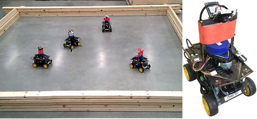
MASTER OF SCIENCE THESIS

                                OF

    RUPASINGHE ARACHCHIGE THIVANKA NYOMAL PERERA

APPROVED:
      Thesis Committee:

              Major Professor   Paolo Stegagno
                                Richard Vaccaro

                                Chengzhi Yuan

                                Brenton DeBoef
                                DEAN OF THE GRADUATE SCHOOL

                UNIVERSITY OF RHODE ISLAND

                                2021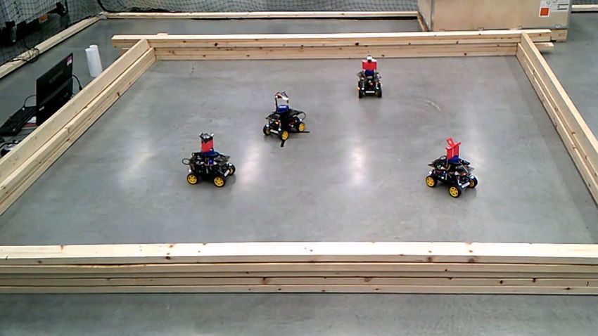
ABSTRACT

    In this thesis, we present a Probability Hypothesis Density (PHD) filter based

relative localization system for robotic swarms. The system is designed to use

only local information collected by onboard lidar and camera sensors to identify

and track other swarm members within proximity. The multi-sensor setup of the

system accounts for the inability of single sensors to provide enough information

for the simultaneous identification of teammates and estimation of their position.

However, it also requires the implementation of sensor fusion techniques that do

not employ complex computer vision or recognition algorithms, due to robots’

limited computational capabilities. The use of the PHD filter is fostered by its

inherent multi-sensor setup. Moreover, it aligns well with the overall goal of this

localization system and swarm setup that does not require the association of a

unique identifier to each team member. The system was tested on a team of four

robots. This thesis content was accepted to DARS-SWARM 2021 conference [1].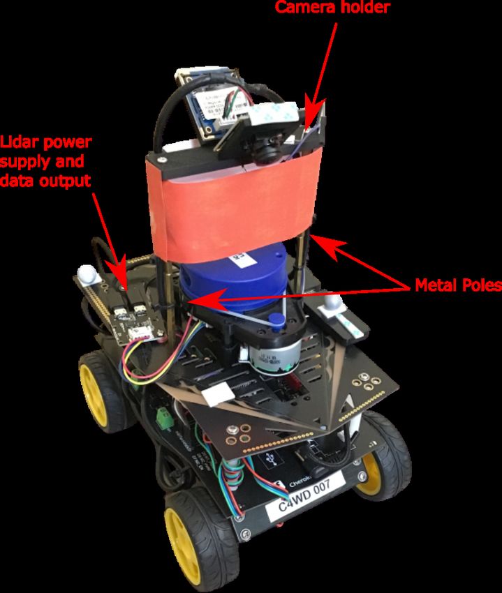
ACKNOWLEDGMENTS

    First and foremost I would like to acknowledge my supervisor and advisor

Professor Paolo Stegagno for his immense support, mentorship during this project

and throughout my graduate career. Thank you for the countless opportunities

you have given me. Additionally, I would like to acknowledge my committe mem-

bers Professor Richard J Vaccaro, Professor Chengzhi Yuan and committee chair

Professor Manbir Sodhi. My sincere thank goes to all the URI staff who have

helped me in many ways to make this research a success.

    I wish to thank my loving wife Nuwanthi for providing me continuous love,

encouragement and support throughout my entire graduate career and beyond.

Without your support, it wouldn’t have been possible. Also, I wish to thank my

parents and my sister for their extended love and support. Finally, I wish to thank

my friends who have been providing their support.

                                        iii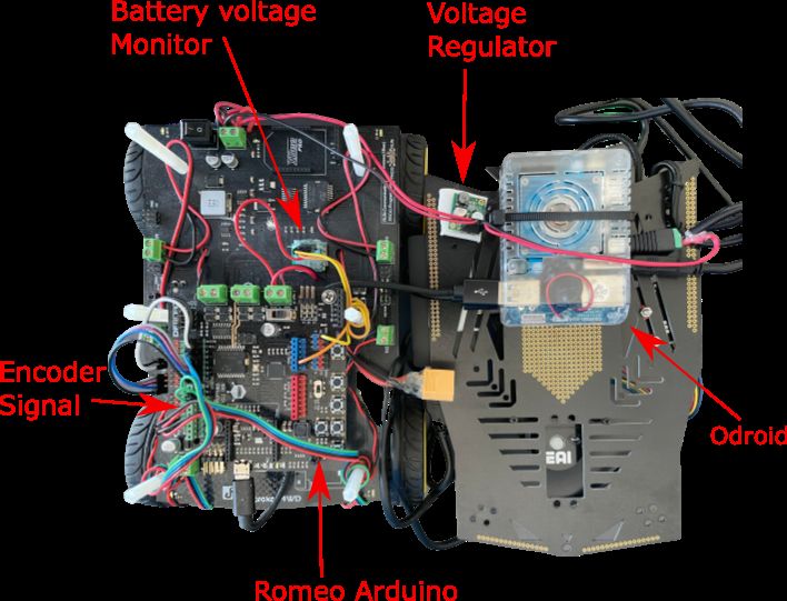
TABLE OF CONTENTS

ABSTRACT . . . . . . . . . . . . . . . . . . . . . . . . . . . . . . . . . .          ii

ACKNOWLEDGMENTS . . . . . . . . . . . . . . . . . . . . . . . . . .                  iii

TABLE OF CONTENTS . . . . . . . . . . . . . . . . . . . . . . . . . .                iv

LIST OF FIGURES . . . . . . . . . . . . . . . . . . . . . . . . . . . . . .          vi

CHAPTER

   1 Introduction . . . . . . . . . . . . . . . . . . . . . . . . . . . . . . .       1

      1.1   Localization methods in a Swarm . . . . . . . . . . . . . . . . .         2

      1.2   PHD filter approach . . . . . . . . . . . . . . . . . . . . . . . . .     4

      1.3   Statement of the problem . . . . . . . . . . . . . . . . . . . . . .      5

   2 Problem Setting and Background . . . . . . . . . . . . . . . . .                 6

      2.1   Multi-sensor PHD filter . . . . . . . . . . . . . . . . . . . . . . .     8

   3 PHD-Filter Based Relative Localization Module . . . . . . . .                   11

      3.1   Time Update . . . . . . . . . . . . . . . . . . . . . . . . . . . .      12

      3.2   Lidar Measurement Update . . . . . . . . . . . . . . . . . . . .         14

      3.3   Camera Measurement Update . . . . . . . . . . . . . . . . . . .          18

   4 Simulation . . . . . . . . . . . . . . . . . . . . . . . . . . . . . . . .      19

      4.1   Simulation results . . . . . . . . . . . . . . . . . . . . . . . . . .   20

   5 Experimental Setup . . . . . . . . . . . . . . . . . . . . . . . . . .          23

      5.1   UGV Platform . . . . . . . . . . . . . . . . . . . . . . . . . . . .     24

      5.2   Main Processing unit . . . . . . . . . . . . . . . . . . . . . . . .     25

                                         iv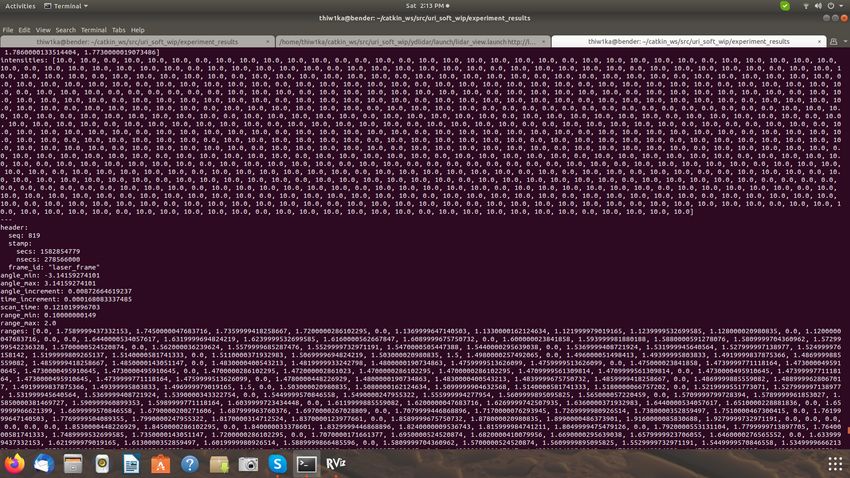
Page
5.3 Odometry system . . . . . . . . . . . . . . . . . . . . . . . . . . 26
5.4 UGV Sensors . . . . . . . . . . . . . . . . . . . . . . . . . . . . 27
5.4.1 Lidar sensor . . . . . . . . . . . . . . . . . . . . . . . . . 28
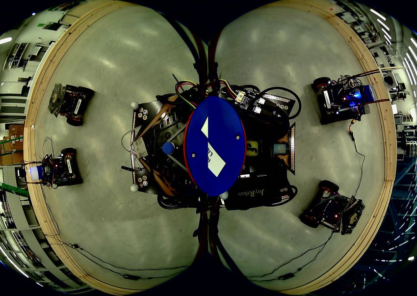
5.4.2 Omni-directional Cameras . . . . . . . . . . . . . . . . . 29
5.5 The testing area . . . . . . . . . . . . . . . . . . . . . . . . . . . 30
5.6 Lidar Measurements . . . . . . . . . . . . . . . . . . . . . . . . 31
5.7 Camera Measurements . . . . . . . . . . . . . . . . . . . . . . . 32
6 Experimental Results . . . . . . . . . . . . . . . . . . . . . . . . . 34
7 Conclusion . . . . . . . . . . . . . . . . . . . . . . . . . . . . . . . . 36
LIST OF REFERENCES . . . . . . . . . . . . . . . . . . . . . . . . . . 37
BIBLIOGRAPHY . . . . . . . . . . . . . . . . . . . . . . . . . . . . . . . 41
v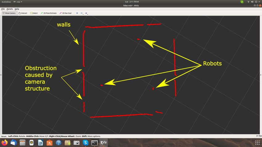
LIST OF FIGURES
Figure Page
1 Left: the robotic swarm used to validate our localization system.
Center: one of the robots used in this work. Right: a representa-
tion of the problem setting: triangles are robots, false positives
are circles, × are lidar measurements lkh , straight dashed lines
are camera measurements chk , blind spots in the lidar measure-
ments are represented as shaded areas. . . . . . . . . . . . . . . 7
2 Filter schematic . . . . . . . . . . . . . . . . . . . . . . . . . . . 11
3 Probaility of Survival Psi . . . . . . . . . . . . . . . . . . . . . . 13
4 Probability of detection for blind spots created by camera struc-
ture . . . . . . . . . . . . . . . . . . . . . . . . . . . . . . . . . 16
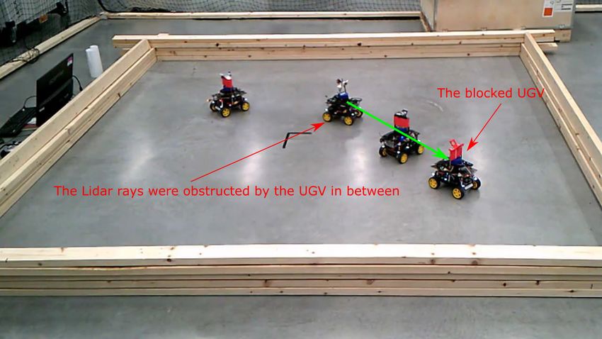
5 Robots block each other . . . . . . . . . . . . . . . . . . . . . . 17
6 Gazebo 20 UGVs simulation . . . . . . . . . . . . . . . . . . . . 19
7 Percentage of time for which each UGV error was greater than
30 cm . . . . . . . . . . . . . . . . . . . . . . . . . . . . . . . . 21
8 No of components estimated by the filter . . . . . . . . . . . . . 22
9 UGV paths during the simulation - LC method . . . . . . . . . 22
10 Final Robot Design . . . . . . . . . . . . . . . . . . . . . . . . . 23
11 Robot Platform - DFRobot Cherokey [2] . . . . . . . . . . . . . 24
12 Inside UGV . . . . . . . . . . . . . . . . . . . . . . . . . . . . . 25
13 Odroid-XU4 . . . . . . . . . . . . . . . . . . . . . . . . . . . . . 25
14 Motor with Encoder . . . . . . . . . . . . . . . . . . . . . . . . 26
15 UGV Front View . . . . . . . . . . . . . . . . . . . . . . . . . . 27
16 YD-Lidar X4 [3] . . . . . . . . . . . . . . . . . . . . . . . . . . 28
17 Camera Sensor . . . . . . . . . . . . . . . . . . . . . . . . . . . 29
vi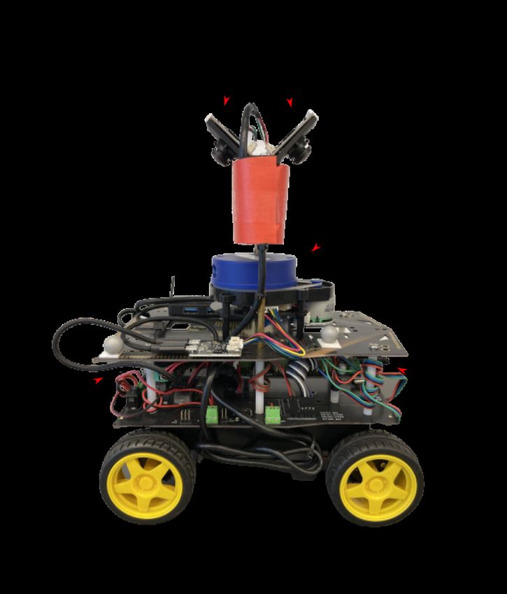
Figure                                                                        Page

  18     Front and rear camera images . . . . . . . . . . . . . . . . . . .       29

  19     Testing area . . . . . . . . . . . . . . . . . . . . . . . . . . . . .   30

  20     Points provided by a typical lidar scan during the experiment.
         visualized using Rviz . . . . . . . . . . . . . . . . . . . . . . . .    31

  21     ROS message - Single Lidar scan . . . . . . . . . . . . . . . . .        32

  22     Image sensor . . . . . . . . . . . . . . . . . . . . . . . . . . . .     33

  23     Distance error of the three UGVs in the LC (left) and LO (right)
         experiments. . . . . . . . . . . . . . . . . . . . . . . . . . . . . .   35

  24     Comparison between the LO and LC experiments. Left: sum of
         the weights of all the components with LO (blue) and LC (red).
         Right: percentage of time that the error on the position of each
         robot is greater than 30cm with LO and LC. . . . . . . . . . . .         35

                                      vii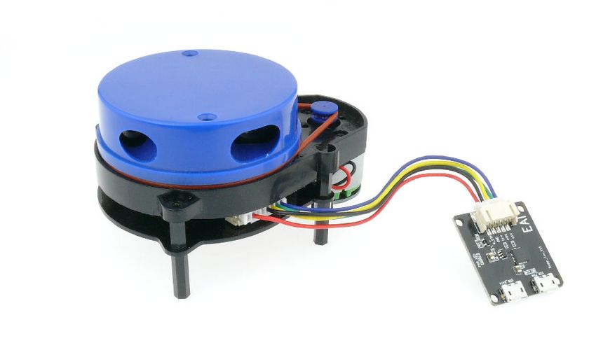
CHAPTER 1

                                  Introduction

    In recent years, robotic swarms have been receiving increasing attention

thanks to many potential applications [4]. Tasks as target search and tracking

[5], search and rescue [6], exploration [7], information gathering, clean up of toxic

spills [8, 9], and construction [10] have been proposed throughout the years.

    A robotic swarm is defined as a group of low cost, relatively simple robots that

intends to perform tasks in an unknown/undiscovered environments. In a swarm,

each individual member performs its own task and collectively the swarm intends

to achieve the main goal.

    Robotics swarms are highly depend on its member locations. Having a cen-

tralised common positioning system for a swarm is not feasible in the above men-

tioned environments, hence each member must have the knowledge of other mem-

bers in its attached frame of reference. This knowledge is gained by utilizing its

own sensors without depending on an external system.

    Most works focus on control algorithms; however, many control laws and

collaborative swarm behaviors require the ability to identify other robots in the

environment, and compute an estimate of their position.

    To retrieve this information many localization algorithms in different oper-

ative conditions have been proposed for multi-robot systems. In cooperative lo-

calization (e.g., [11]), the robots communicate each other’s odometry and relative

measurements to compute the location of each team member in a common frame

of reference, usually through an online Bayesian filter (e.g., [12, 13]) or estimator

(e.g., [14]). However, the assumption of a common frame of reference accounts as

a form of centralization and should be avoided in a robotic swarm setting.

                                         1
1.1 Localization methods in a Swarm
In relative localization algorithms, the assumption of a common frame of ref-
erence is eased and the goal of each robot is to estimate the pose of other robots
in its attached frame of reference. This has been addressed through Bayesian fil-
ters [15], geometrical arguments [16], or a combination of both [17]. Usually, both
relative and cooperative localization algorithms require not only some position,
bearing or distance measurements, but also that each measurement comes with
the unique identifier of the measured robot. However, unique identification of each
robot could be difficult or undesirable. Typical approaches include visually tagging
each robot and extracting the tag through cameras [18], using dedicated infrared
systems [19] or RFIDs [20]. Tagging and ID exchange in many cases are not viable
solutions. It could be technically unfeasible, particularly in case of large numbers
of robots or with sensors, as laser scanners, that do not allow for unique identifi-
cation capabilities. It also accounts as a form of centralization, meaning that all
robots need to know the same set of IDs. Last but not least, it may jeopardize the
task to make explicit the identity of each robot, if the swarm is for example in an
escorting or disguising mission.
In a number of papers, the problem of computing an estimate of other robot’s
location with untagged measurements has been referred to as localization with
anonymous measurements [17, 21], or unknown data association. In [21], using
odometry and untagged relative measurements communicated from other robots,
the robots were able to produce tagged (i.e., associated with a unique identifier)
relative pose estimates.
However, associating ids to each robot is not a mandatory condition to per-
form cooperative tasks as formation control [22], encircling [23], and connectivity
maintenance [24], as long as each robot is able to identify that some entities in the
2environment are generically teammates, and compute an estimate of their relative
positions. Moreover, in a robotic swarm setup, robots could have limited or no
communication capabilities, and should rely only on local self-gathered measure-
ments to perform their tasks.
In this situation, the choice of the sensor equipment endowed to the robots
becomes even more crucial. On the one hand, the sensors should provide enough
information to allow (non-unique) identification of other robots, and quantita-
tive estimation of their relative position. On the other hand, robotic swarms are
usually composed of relatively small and cheap robots, featuring limited computa-
tional capabilities that are not compatible with expensive informative rich sensor
equipment. Single sensor approaches are limited by the sensing technology. Using
distance sensors as lidars, robots can be easily mistaken for obstacles of similar
size, and vice versa. On the other hand, camera sensors would be able to iden-
tify robots more reliably, but they would directly provide only bearing information,
and distance estimates could be affected by consistent noise, have long convergence
time, and require persisting excitation conditions [25, 26]. RGB-D sensors offer
the best of both worlds but usually have limited fields of view, while the robots
should be aware of teammates and obstacles in entirety of their surroundings.
31.2 PHD filter approach
Given the multi-target multi-sensor tracking nature of the proposed problem,
a natural choice would be the employment of a Probability Hypothesis Density
(PHD) filter. The PHD filter was first proposed in [27] as a recursive filter for
multi-target multi-sensor tracking. The filter in its theoretical form would require
infinite computational power. However, some authors have proposed Gaussian
mixture [28] and particle based implementations [29] among others.
PHD filters have already been employed in multi-robot localization. In [30],
the authors presented a PHD filter to incorporate absolute poses exchanged by
robots and local sensory measurement to maintain robots’ formation when com-
munication fails. In [31], a team of mobile sensors was employed to cooperatively
localize an unknown number of targets via PHD filter. However, in these two
works a common frame of reference was assumed, which is not compatible with
our setup. In [32], the authors implemented a PHD filter to fuse ground robot
(UGV) odometry and aerial camera measurements to estimate the location and
identity of the UGVs. However, only the aerial robot computes the position of
the other robots, and not every team member. In [33], the authors used two dif-
ferent visual features to describe the target of interest enhancing the PHD-based
tracking. However, this is an example of video tracking and the metric pose of the
targets are not estimated. Therefore, none of the setups discussed in literature is
compatible with the needs of a robotic swarm and our settings.
41.3 Statement of the problem
In this thesis we propose a multi-model approach in which we employ multiple
sensors, fisheye cameras and laser scanners, to combine the recognition capability
of the first with the accuracy of the second. However, this approach requires
non-trivial data fusion techniques. Hence we propose a novel robo-centric imple-
mentation of the PHD filter for the fusion of lidar and camera measurements in a
swarm setup.
The proposed filter design runs independently on each robot to compute es-
timates of other teammates position in its attached frame of reference. The mea-
surements for the filter will be obtained using on-board lidar and camera sensors
and will not depend on any external sensor data. The filter computations are done
in the on-board main processing unit, which computes estimates in real time.
The filter will be first tested in a simulated robotic swarm where each swarm
member is equipped with above mentioned sensors. Then we develop a UGV (Un-
manned ground vehicle) to test the filter in a real robotic swarm. Each UGV will
be equipped with said sensors and a processing unit as per filter requirement. The
issues that arose during the experiment will be investigated and will be addressed
by modifying filter parameters.
5CHAPTER 2
Problem Setting and Background
The system we consider (Figure 1) consists of n UGVs {R1 , R2 , ..., Rn } in a
2D space, with n unknown and time-variant. The generic robot Rj is modeled as
a rigid body moving in 2D space and is equipped with an attached reference frame
Fj = {Oj , Xj , Yj } whose origin coincides with a representative point of the robot.
Let qhj ∈ R2 be and ψhj ∈ SO(1) respectively the position and orientation of Rh in
Fj , and let ojh be the position of Oh in Fj . In the following, we indicate with R(φ)
the elementary 2D rotation matrix of an angle φ:
cos(φ) −sin(φ)
R(φ) = . (1)
sin(φ) cos(φ)
Robot Rj is equipped with multiple sensors. First, the odometry module of
Rj provides, at each time k, a measurement Ukj = [∆xjk ∆ykj ∆ψkj ]T ∈ R2 × SO(1)
of the robot linear and angular displacement between two consecutive sampling
instants k − 1 and k on the XY plane.
Rj is also equipped with a lidar sensor. Lidar measurements are processed
with a feature extraction algorithm that identifies all objects in the scan (includ-
ing robots) whose size is comparable with the size of the robots. In general, we
assume that there is an unknown number of objects in the environment that will
be detected in the lidar as possible robots. Therefore, at each time step k the
algorithm provides a set of lk relative position measurements Lk = {lk1 , ..., lklk } in
Fj , representing the position of robots or obstacles in the field of view of the sen-
sor. The sensor is affected by false positive (some measurements may not refer to
actual objects) and false negative measurements (some object or robot may not be
detected) due to obstructions and errors of the feature extraction algorithm.
6lidar field of view
blind spot
due to
obstruction
false
positive
lidar
measurements
camera
measurements
blind spots due to
camera holders
Figure 1: Left: the robotic swarm used to validate our localization system. Center:
one of the robots used in this work. Right: a representation of the problem setting:
triangles are robots, false positives are circles, × are lidar measurements lkh , straight
dashed lines are camera measurements chk , blind spots in the lidar measurements
are represented as shaded areas.
Lastly, two fisheye cameras are mounted on Rj , one oriented towards the front
of the robot, and one towards the back. This setup allows us to identify robots in
a 360◦ field of view. The images from the cameras are processed using a feature
extraction algorithm that has the capability of identifying a generic robot based
on color. The algorithm does not uniquely identify and label each robot. At time
step k, the cameras provide a set of ck bearing measurements Ck = {c1 , ...cckk } in
Fj . Also in this case, there may be false positive (non-robots identified as robots)
and false negative (missed robot detections) measurements. In the following, the
camera and lidar measurements collected at time k will be denoted together as
Zk = {Lk , Ck }. Note that camera and lidar have different rates and in general are
not synchronized. Therefore, without loss of generality, for some k it may be either
Lk = ∅, or Ck = ∅, or both. A representation of all sensor readings is provided in
Figure 1.
The objective of Rj is to compute at each time step k an estimate of the
number n(k) and positions of all robots in the environment.
72.1 Multi-sensor PHD filter
This Section provides the necessary background on the PHD filter and is
mostly based on [27, 28, 29]. Assuming that there are n (with n unknown and
variable over time) targets living in a space X , the goal of the standard PHD filter
is to compute an estimate of the PHD of targets in X . The PHD fk (x) at time
k is defined as the function such that its integral over any subset S ⊆ X is the
R
expected number of targets N (S) in that subset, i.e., N (S) = S fk (x)dx.
The PHD filter is a recursive estimator composed of two main steps: a time
update and a measurement update. The time update is meant to produce a pre-
diction of the PHD fk|k−1 (x) at time step k given the estimate fk−1|k−1 (x) at time
k − 1, through the time update equation:
Z
fk|k−1 = bk|k−1 (x) + [Ps (x0 )fk|k−1 (x|x0 ) + bk|k−1 (x|x0 )]fk−1|k−1 (x0 )dx0 (2)
where bk|k−1 (x) is the probability that a new target appears in x between times
k − 1 and k, Ps (x0 ) is the probability that a target in x0 at time k − 1 will survive
into step k, fk|k−1 (x|x0 ) is the probability density that a target in x0 moves to x,
and bk|k−1 (x|x0 ) is the probability that a new target spawns in x at time k from a
target in x0 at time k − 1.
Note that both fk−1|k−1 (x) and fk|k−1 (x) are computed considering only the
measurements up to time k − 1. Measurements Zk collected at time k are incorpo-
rated in the estimate through the measurements update to compute the posterior
PHD:
fk|k (x) =
" #
X PD (x)g(z|x)
fk|k−1 (x) 1 − PD (x) + R (3)
z∈Zk
λc(z) + PD (x0 )g(z|x0 )fk|k−1 (x0 )dx0
where PD (x) is the probability that an observation is collected from a target with
state x, g(z|x) is the sensor likelihood function, and λc(z) expresses the probability
8that a given measurement z is a false positive.
Although elegant, equations (2) and (3) cannot be implemented in practice
for generic functions. A popular approximation, the Gaussian Mixture PHD filter
(GM-PHD) considers all PHD functions fk−1|k−1 (x), fk|k−1 (x), and fk|k (x) to be
sums of weighted Gaussian functions in the form:
X X
i i
f∗|∗ (x) = f∗|∗ (x) = w∗|∗ N (x; mi∗|∗ , pi∗|∗ ) (4)
i i
i i
where f∗|∗ (x) is the generic i-th component, w∗|∗ , mi∗|∗ , and pi∗|∗ are respectively
the weight, mean and covariance matrix of the i-th component. Introducing the
GM representation (4) in equation (2), and assuming that the probability of sur-
vival can be approximated as a constant for each component (Ps (x0 ) ' Psi ), the
spawning probability bk|k−1 (x|x0 ) is zero, and the system model fk|k−1 (x|x0 ) and
target birth probability bk|k−1 (x) are Gaussian functions, the GM-PHD filter time
update equation becomes:
X Z
fk|k−1 = bk|k−1 (x) + i
wk−1|k−1 Psi fk|k−1 (x|x0 )fk−1|k−1
i
(x0 )dx0 (5)
i
Therefore, the PHD prediction will have a component for each component in the
PHD posterior fk−1|k−1 (x). Moreover, the integral term will be the same as a
prediction step of the standard Kalman filter, so every component of fk|k−1 (x) will
be a Gaussian function, and it will be possible to compute the PHD prediction by
simply applying component-wise the time update of a Kalman filter.
Introducing the GM representation (4) in equation (3), assuming that the
probability of detection can be approximated as a constant PD (x) ' PDi for each
i
component fk+1|k (x), and c(z) = 0, the GM-PHD filter measurement update equa-
tion becomes:
X
i
XX PDi fk|k−1
i
(x)g(z|x)
PDi
fk|k (x) = fk|k−1 (x) 1− + P R . (6)
i i z∈Zk i PDi g(z|x0 )fk|k−1
i
(x0 )dx0
9i
showing that, if Zk contains m measurements, each component fk|k−1 (x) generates
m + 1 components in fk|k (x). Moreover, if g(z|x) is a Gaussian function, the last
term is a sum of Gaussian functions, each function being the result of a single-
component Kalman filter measurement update step.
An additional pruning step is needed to limit the number of components in the
PHD. In fact, if all components were kept at each time step, their number would
grow exponentially with the number of measurements. Therefore, all components
whose weight is below a given threshold at the end of the measurement update are
eliminated.
It is clear from its formulation that the PHD filter is inherently multi-sensor.
In fact, when multiple sensors are present, multiple measurement updates can be
applied consecutively, each one as a component-wise Kalman filter update step.
10CHAPTER 3
PHD-Filter Based Relative Localization Module
Prior Estimate
Time step (t‐1)
Time Update using
Odometry
New Lidar
Lidar Measurement Measurement
Update available
Yes
No
New Camera
Camera Measurement
Measurement Update available
Yes
No
Final Estimate
Time step (t)
Figure 2: Filter schematic
Following the scheme presented in the Section 2.1, our localization module
consists of a time update step and two measurement update steps. Note that
the module is asynchronous, so there is no particular order or sequence in which
these steps are performed. While the time update is periodically performed, the
measurement updates are performed if and when measurements become available.
11The estimated state of the target robots is their position in Fj , mik|k = q∗j (k) ∈ R2 ,
where the ∗ expresses the concept that the i-th component may refer to any of the
tracked target robots. The covariance of mik|k is therefore pik|k ∈ R2×2 .
3.1 Time Update
During the time update, the owner’s Rj odometry Ukj = [∆xjk ∆ykj ∆ψkj ]T is
used to update the mean and covariance of all components of the PHD. The k th
time update for the generic ith component is given by:
mik|k−1 = R(∆ψkj )(mik−1|k−1 − [∆xjk ∆ykj ]T ) (7)
T T
pik|k−1 = R(∆ψkj )pik−1|k−1 R(∆ψkj ) + R(∆ψkj )Qk−1 R(∆ψkj ) (8)
i
wk|k−1 = Psi wk−1|k−1
i
(9)
where Psi is the survival probability from time step k − 1 to the time step k of the
ith component fk−1|k−1
i
, and Qk−1 is the system noise.
Ideally, the survival probability Psi , depends on the real probability that a
target disappear. In a robotic swarm context, this probability would be extremely
low in the whole domain. Therefore, we have used it as a design parameter to meet
the objectives of the localization module. Coherently with the task and motivation
of this thesis, only local information is required and available to each robot. Using
Psi , we prefer to let too far components fade. At this aim, we use an inverse sigmoid
function (Figure 3) to compute Psi :
1
Psi = i (10)
(1.05 + e4(||mk−1|k−1 ||−4) )
This creates a circular area in around Rj in which it tracks other robots. To
account for targets that enters into this area from outside, a birth target component
bk|k−1 (x) is added at each time update, such that its mean, covariance and weight
121
0.9
0.8
0.7
Survival Probaility Ps
0.6
0.5
0.4
0.3
0.2
0.1
0
0 1 2 3 4 5 6 7 8 9 10
Distance (m)
Figure 3: Probaility of Survival Psi
are respectively:
b b 4 0
, wb = 0.001
m = 0 0 , p = (11)
0 4
The assigned weight is very low so if there is no correspondence with the measure-
ments (i.e., at least one measurement without a good correspondence with one or
more components of the PHD prior), bk|k−1 (x) will be pruned immediately. The
choice of limiting the area in which each robot tracks its teammates is also bene-
ficial for the scalability of the method. In fact, even if the swarm was comprised
of hundreds of agents, each robot would only track the ones that are closer to it,
therefore linking the computational complexity of the filter to the density of the
swarm rather than to the total number of robots.
133.2 Lidar Measurement Update
After the time update, the lidar measurement update is performed only when
new measurements are available. We assume that the lidar at time k collect lk
position measurements lkh ∈ Lk , h = 1, ..., lk in Fj . Following equation (6), each
i i(l +1) i(l +1)+h
component fk|k−1 of fk|k−1 generates lk + 1 components fk|kk , fk|kk , h =
i(l ) i(l )
1, ..., lk in fk|k . One component fk|kk+1 has the same mean mk|kk+1 = mik|k−1 and
i(l )
same covariance pk|kk+1 = pik|k−1 of the original component, while the weight is
updated as:
i(l +1)
wk|kk = (1 − L Pdi )wk|k−1
i
(12)
where L Pdi is the probability that a target corresponding to component fk|k−1
i
is
detected by the lidar. The other lk components are created using measurement
update equations of the Kalman filter:
i(l +1)+h
mk|kk = mik|k−1 +L Kki (lkh − mik|k−1 ) (13)
i(l +1)+h
pk|kk = (I −L Kki L Hk )pik|k−1 (14)
i(l +1)+h
wk|kk = L Pdi wk|k−1
i
N {lkh ; mik|k−1 , pik|k−1 } (15)
where L Hk is the lidar observation matrix and Kk is the associated Kalman gain:
1 0
L
Hk = L
Kki = pik|k−1 L HkT (L Hk pik|k−1 L HkT + L Rk )−1 (16)
0 1
where L Rk is the covariance of the noise on the lidar measurements, that is deter-
mined experimentally as:
L 0.0025 0
Rk = (17)
0 0.0025
The probability of detection L Pdi is a key parameter for the success of the
i
filter. For each component fk|k−1 ,L Pdi is calculated considering four factors that
limit the lidar sensor ability to detect objects. Distance, blind spots caused by the
14camera holders, obstruction of a robot by another robot, and interference caused
by other lidar sensors. The final L Pdj is the product of all those factors:
L
Pdj =L Pd|dis
i
∗L Pd|cs
i
∗L Pd|b
i
∗L Pd|in
i
(18)
i
The first factor is the distance of each component fk|k−1 which is related to
the lidar sensor range. If a component is located beyond the range of the lidar,
then it will not be detected. In our particular case, the range of the lidar is limited
to 2m. A sigmoid function was used to calculate L Pd|dis
i
:
L i 1
Pd|dis = i
(19)
1.02 + e8∗(||mk+1|k ||−1.5)
The second factor is due to the two pillars that support the fish eye cameras on
Rj , that create four blind spots in the field of view (FOV) of the lidar, whose centers
αi , i = 1, . . . , 4 and angular width βi , i = 1, . . . , 4 were determined experimentally.
i
Denoting with θk|k−1 the bearing angle of the mean of the i-th component, a sum
of Gaussian functions is implemented to calculate L Pd|cs
i
(Figure 4):
4
X
L j i
Pd|cs = 1 − N {θk|k−1 ; αi , βi /2} . (20)
i=1
The third factor L Pd|b
i
models the situation in which robots block each other
from the FOV of the lidar, that is therefore unable to collect a measurement for
the robot that is behind. Similar situation seen in Figure 5. Hence the probability
of detection of each component is reduced incorporating a zero mean Gaussian
function L Pd|b
i
based on i) the angle difference θdif f between pairs of components;
and ii) their Euclidean distance ||mik+1|k || from Rj . When θdif f becomes close to
zero for some pair, the robot which has the shortest Euclidean distance from Rj
i
will block the other robot. For the generic component fk+1|k (x), using all the
components, L Pd|b
i
is calculated as:
151
probability for blindspots by camera structure
0.9
0.8
0.7
0.6
0.5
0.4
0.3
0.2
0.1
0
-150 -100 -50 0 50 100 150
Angle -180 to 180 (Degrees)
Figure 4: Probability of detection for blind spots created by camera structure
j i
θdif f = |θk|k−1 − θk|k−1 | (21)
X j
L i
Pd|b = (1 − wk|k−1 N (θdif f ; 0, 3deg)) (22)
∀{i,j}:||mjk|k−1 ||ϑ = 0, 0.5, . . . , 360. Therefore we used the intensity readings to calculate L Pd|in
i
for
i
fk+1|k (x):
i ϑ 2
L i
X 1 − 0.6 ∗ e−(θk|k−1 −∠lint )
Pd|in = (23)
ϑ =0,ϑ=0,0.5,...360}
2 ∗ c2
∀{lint
ϑ
where c denotes the covariance of each lint = 0.
Figure 5: Robots block each other
173.3 Camera Measurement Update
Similar to the lidar measurement update, the camera update is performed only
when new camera measurements Ck = {c1k , ...cckk } are available. Each c1k is provided
as a 2D normalized vector pointing in the direction of a target. Following equation
i
(6), each component fk|k−1 generates ck + 1 components in fk|k . As for the lidar
i(c +1) i(c +1)
measurements, one component fk|kk has the same mean mk|kk = mik|k−1 and
i(l )
covariance pk|kk+1 = pik|k−1 of the original component, while the weight is updated
as:
i(ck +1)
wk = (1 − C Pdi )wk|k−1
i
(24)
The other ck components are computed using the Kalman filter equations:
i(c +1)+h
mk|kk = mik|k−1 + C Kki (chk − mik|k−1 ) (25)
i(c +1)+h
pk|kk = (I − C Kki C Hk )pik|k−1 (26)
i(c +1)+h
wk|kk = C Pdi wk|k−1
i
N {chk ; mik|k−1 , pik|k−1 } (27)
where C Pdi is the camera probability of detection, Hk is the observation matrix,
and Kk is Kalman gain:
!
−y i xi
Hk = , Kki = pik|k−1 HkT (Hk pik|k−1 HkT + C Rk )−1 (28)
||mik|k−1 || ||mik|k−1 ||
where mik|k−1 = [xi y i ]T and C
Rk = 25deg is the covariance of the noise of the
camera measurements.
The probability of detection C Pdi is computed as the product of two factors,
distance from Rj and obstruction of a robot by another robot:
C
Pdi = C Pd|dis
i
∗ C Pd|b
i
(29)
The first factor is computed with an inverse sigmoid function:
C i 1
Pd|dis = (30)
5∗(||mjk+1|k ||−4)
(1.1 + e )
while for the second factor, C Pd|b
i
= L Pd|b
i
.
18CHAPTER 4
Simulation
Figure 6: Gazebo 20 UGVs simulation
The filter was first tested in simulation before testing in real robot experiment.
A swarm of UGVs was simulated in Gazebo/ROS. The UGV model was equipped
with a simulated lidar sensor. The implementation of a fish-eye camera was difficult
due to unavailability of its manufacture parameters and the computational load of
simultaneously simulating 10 -20 camera sensors, hence the camera measurements
were generated directly using the UGV locations. A zero mean Gaussian noise was
added to the camera measurements to simulate realistic measurements.
Figure 6 shows the typical simulation setup with a 6m x 6m square testing
area with walls to keep the UGVs in close proximity to each other. The experiment
consists of 20 UGVs where a single UGV executes the filter to estimate the position
of other 19 UGVs. All UGVs perform a pseudo random motion with obstacle
avoiding capabilities. In Figure 6 the red colored UGV performs the filter and its
19knowledge is visualized in the visualizer window on the left side. The visualizer
was developed in openCV to interpret the filter output and simplify the debugging
process. Additionally, it visualizes the measurements provided by the sensors. The
Visualizer provides 360 degree view around the UGV with the 2m range in each
side. 2 meters was considered as the lidar sensor range and 3m for the camera
sensor. In the Visualizer, the symbol ’x’ shows the lidar measurement, arrows
represents the bearing measurements from the camera and the circles show the
weight of each component of the estimated PHD. The experiment was conducted
for 300 seconds and the filter results were recorded to a ROS bag. The ROS bag
was later analysed using Matlab software to generate the plots.
4.1 Simulation results
Three plots were generated using simulated results to evaluate the performance
of the filter and illustrate the benefits of the proposed multi-sensor approach. The
multi-sensor approach was compared by running the filter with (Lidar+Camera -
LC) and without camera measurements (Lidar only - LO).
The bar chart in Figure 7 represents the percentage of time for which each
UGV error was greater than 30 cm only considering the time when the UGV was
within the sensor range. The filter estimates was compared with the actual UGV
locations provided by the simulator to compute the error. Overall out of 20 UGVs
only four UGVs had the error greater than 25 percent in LC method and 9 robots
in LO. It is well seen in the Bar chart that LC method performs well compared to
LO method.
Figure 8 represents the total sum of the weight of all components with respect
to the time during the whole experiment. The filter estimated in average 15 UGVs
in the duration of the simulation using LC method.
In Figure 9 the plot shows the path for each UGV during the simulation when
2070
LO Method
LC Method
60
50
Error Percentage %(s)
40
30
20
10
0
0 2 4 6 8 10 12 14 16 18 20
Robot ID
Figure 7: Percentage of time for which each UGV error was greater than 30 cm
LC method used. The symbol ’x’ represents the mean of the components computed
by the filter. At each time step, the UGV path and the relevant estimates were
plotted. Overall the filter was able to follow an accurate path of the UGVs. Note
that the UGV paths that are not near estimates refers to UGV that were out of
the sensor range during that time step.
2150
LO method
45 LC method
40
Sums of weights 35
30
25
20
15
10
5
0 50 100 150 200 250 300
Time (s)
Figure 8: No of components estimated by the filter
Robot 1
2
Robot 2
Robot 3
Robot 4
1.5
Robot 5
Robot 6
Robot 7
1
Robot 8
Robot 9
Robot 10
0.5 Robot 11
Robot 12
y Coordinates (m)
Robot 13
0 Robot 14
Robot 15
Robot 16
-0.5 Robot 17
Robot 18
Robot 19
-1 Robot 20
-1.5
-2
-2.5
-3
-3 -2 -1 0 1 2 3
x coordinates (m)
Figure 9: UGV paths during the simulation - LC method
22CHAPTER 5
Experimental Setup
The relative localization system has been tested in robot experiments with four
Unmanned Ground Vehicles (UGV). During a typical experiment, the UGVs will
run a simple pseudo-random motion with obstacle avoidance. All computations
are done on the on-board Odroid and using on-board sensors. Similar to the
simulation, one UGV performs the estimation algorithm and the final estimates
were published on a ROS topic and recorded to a ROS bag along with ground
truth provided by an Optitrack motion capture system.
Figure 10: Final Robot Design
Figure 10 shows the final design of the UGV that is used for the experiment.
The design consist of a four-wheeled base equipped with two Omni-directional
23cameras, one Lidar sensor, a main processing unit, a lower level processing unit,
wheel encoders and a 12V battery pack to provide power. Additionally each UGV
was retrofitted with a red color strip on the camera structure to improve the
detection in camera measurements.
5.1 UGV Platform
The UGVs were constructed using a commercially available four wheeled dif-
ferential drive robot platform, the DFRobot Cherokey (22.5cm x 17.5cm). Each
UGV is equipped with wheel encoders and a Romeo V2 (an Arduino Robot Board
(Arduino Leonardo) with Motor Driver). The Romeo V2 processes and executes
the low level control to follow desired velocity commands.
Figure 11: Robot Platform - DFRobot Cherokey [2]
The DFRobot Cherokey has two levels in its platform. The lower level plat-
form is embedded with motor controllers and the power distribution for the motors.
The space between two levels is utilized to accommodate the Battery pack, main
processing unit, voltage divider circuits and Arduino robot board. The top level
is utilized to attach the three sensors.
245.2 Main Processing unit
Figure 12: Inside UGV
For processing higher level tasks, an Odroid-XU4 - a small single board com-
puter - is mounted on the robot. The Odroid-XU4 hosts an Exynos5422 Cortex™-
A15 2Ghz Quad core and a Cortex™-A7 1.5Ghz Quad core CPUs with Mali-T628
MP6 GPU [34]. The Odroid runs a GNU-Linux OS along with Robot Operating
System (ROS) to manage sensor data collection and real time processing.
Figure 13: Odroid-XU4
255.3 Odometry system
The odometry system was implemented to compute the displacement of the
robot. The displacement during a given time period is required to compute the time
update of the filter. The implementation of the odometry was done by counting the
impulses provided by the motor encoders for a given time period. The encoders are
connected to Romeo Arduino board’s interrupt pins to count the received impulses.
Figure 14: Motor with Encoder
For a single motor revolution, the encoder provides 16 pulses. The 120:1
gear box attached to the motor increases the encoder pulses to 1920 per wheel
revolution. By counting the pulses Pt at time t, the linear displacement Dt and
Angular displacement θt is given by:
π ∗ 2 ∗ rw ∗ 0.5 ∗ (PtL + PtR )
Dt = (31)
1920
π ∗ 2 ∗ rw ∗ (PtL − PtR )
θt = (32)
1920 ∗ wax
where PtL , PtR are pulses of the left side motor and pulsars of the right side motor,
rw is the wheel radius, and wax is the UGV axis width.
265.4 UGV Sensors
Each UGV is equipped with a Lidar and two omni directional cameras that
are integrated to have 360 degree field of view. All three sensors are connected to
the Odroid using standard USB ports. Both the lidar and the cameras are fixed
in the origin Oj of Fj and aligned with the X axis, eliminating rotational and
translational complexities during the image and scan processing.
Figure 15: UGV Front View
275.4.1 Lidar sensor
The Lidar model XU4 from YDLidar was selected as the lidar sensor for
the UGV. The XU4 is a low-cost, light-weight, belt driven, two dimensional range
finder. It can provide range information up to 10m in all 360 degrees at 7 Hz frame
rate. For a single revolution it provides 720 range data points with the resolution
of data point per 0.5 degree. The lidar is mounted on the center of the top platform
to align with the UGV’s frame of reference system. A ROS software package is
provided with the lidar that publishes the scan data. A separate algorithm was
developed to read scan data from the ROS topic and search for other UGVs.
Figure 16: YD-Lidar X4 [3]
285.4.2 Omni-directional Cameras
The two cameras are standard USB web cameras equipped with a 180 degree
fish-eye lens. Each camera provides two megapixel 1920x1080 resolution images at
30 fps rate.
Figure 17: Camera Sensor
A camera holder was designed and 3D printed to hold the cameras above
the lidar at an height of 130mm from UGV and a 45 downward degree angle.
This specific height and angle is designed to maximize the horizontal FOV of the
combined camera images.
All the UGVs have been equipped with a red strip around the camera holder
in order to allow camera tracking via color extraction.
Figure 18: Front and rear camera images
295.5 The testing area
The testing area is a 3m x 3m square space with raised walls to avoid distur-
bances from the external environment and keep the robots in proximity of each
other. However, it is also larger than the FOV of the lidar to allow robots to exit
and re-enter the tracking radius. Ground truth of the actual position of the robots
is provided at each time by an Optitrack 6Dof motion tracking system.
Figure 19: Testing area
305.6 Lidar Measurements
An algorithm was developed to obtain each lidar scan published in the ROS
topic and search for other UGV. During a typical lidar scan, the laser beam is
reflected when it hits on other UGV’s lidar structure which has a shape of a circle.
As seen in Figure 20 each UGV was represented by small set of points, which
has a shape of an arch when inspected closely. Arc lengths of these points were
computed and compared with the diameter of lidar structure to distinguish UGVs
from larger obstacles. The measured diameter of typical lidar structure is 65mm.
Figure 20: Points provided by a typical lidar scan during the experiment. visualized
using Rviz
The arc lengths which were less than 65mm were extracted as the possible
measurements for other UGVs. Range and bearing for these possible measurements
were translated into Cartesian coordinates, rotated to UGV frame of reference and
provided as the lidar measurements to the filter.
31Figure 21: ROS message - Single Lidar scan
5.7 Camera Measurements
The camera measurement are generated using a color extraction method. The
color extraction algorithm first defines the boundaries for RGB (Red, Green, Blue)
color space to filter the red color. When an image is received from an UGV camera,
it is sent through the color filter to eliminate other colors except red. The remaining
red color blobs were extracted and their pixel coordinates are used to compute the
bearing measurements.
Spherical coordinate system was used to compute the angular measurements
from the pixel coordinates. Given pixel coordinate xp , yp for an identified blob,
pixel distance Ds between sensor and fish eye lens, the angular measurement in
camera frame of reference c θ1 :
32Lens
Distance from sensor to lens
sn
loe
ro t
sn
es
m
or
ec f
at n
siD
Polar angle
Z Y
p
Azemuth Xp,Y
X angle
nsor
g e se
Ima
Figure 22: Image sensor
p
θazimuth = xp 2 + y p 2 (33)
p
xp 2 + y p 2
θpolar = arcsin( ) (34)
Ds
xc sin θpolar ∗ cos θazimuth
yc = sin θpolar ∗ sin θazimuth (35)
zc cos θpolar
ZR1 j = RcRj ∗ Zc (36)
c 1 y Rj
θ = arctan (37)
xR j
R
Where Rc j is the rotational matrix from camera frame of reference to UGV
frame of reference and yRj ,xRj are the coordinates in UGV frame of reference.
Figure 22 shows the geometric argument for the sensor and the lens.
33CHAPTER 6
Experimental Results
The experimental data was analysed in Matlab software to highlight the ben-
efit of the proposed multi-sensor approach with (Lidar+Camera - LC) and without
(Lidar only - LO) providing the camera measurements.
Figure 23 shows the distance error for each robot from the closest component
whose weight is greater than 0.1. Overall, the LC method performs well except
for some instants near time 150s and 190s in which the robot performing the
estimate was consistently in a corner of the arena, hence with a limited field of view,
effectively leading to robot’s UGV 07 position not being measured for several tens
of seconds. The plots show also that the LC method outperforms the LO method
being able to keep the error bounded for most of the time when measurements are
available.
A numerical comparison between the LC and LO methods is provided in
Figure 24. In order to quantify the better performance of the LC filter, we have
computed the percentage of time for which each robot’s distance error is greater
than 30cm. The values, reported in the table in Figure 24(left), show how the
employment of camera measurements in addition to the lidar greatly reduces the
error time of a factor 2 to 5. Finally, in Figure 24(right) we report the total sum
of the weight of all components with respect to time during the whole experiment.
From this plot, it is possible to establish that the LC method is more effective in
correctly estimating the number of robots, and therefore in eliminating estimates
that refer to objects in the environment and not robots.
342 2
UGV 07 UGV 07
1.8 UGV 02 1.8 UGV 02
UGV 10 UGV 10
1.6 1.6
min(|Ground Truth - mik|) in m
min(|Ground Truth - mik|) in m
1.4 1.4
1.2 1.2
1 1
0.8 0.8
0.6 0.6
0.4 0.4
0.2 0.2
0 0
0 50 100 150 200 250 0 50 100 150 200 250
Time (s) Time (s)
Figure 23: Distance error of the three UGVs in the LC (left) and LO (right)
experiments.
20
L
18 LC
16
14
sum of the weights
12 Method LO LC
10 UGV 07 20.7% 12.7%
8 UGV 02 10.9% 2.6%
6 UGV 10 1% 0.2%
4
2
0 50 100 150 200 250
Time (s)
Figure 24: Comparison between the LO and LC experiments. Left: sum of the
weights of all the components with LO (blue) and LC (red). Right: percentage of
time that the error on the position of each robot is greater than 30cm with LO
and LC.
35CHAPTER 7
Conclusion
In this thesis we have presented a multi-sensor relative localization system
for robotic swarms based on the PHD filter. Our system has been tested with
real robot experiments, and evaluated against a single-sensor method based on the
same principle. The results show that the multi-sensor approach performs better
than the single-sensor method.
In the future, on the one hand we plan on improving the relative localization
and include negative information measurements to simultaneously track robots
and obstacles. On the other hand, we plan to pair the localization system with a
decentralized formation control methods to perform real-world tasks as exploration,
SLAM, patrolling and human-swarm interaction.
36LIST OF REFERENCES
[1] R. T. Perera, C. Yuan, and P. Stegagno, “A phd filter based localization
system for robotic swarms,” in Proceedings DARS-SWARM2021 conference,
June 2021.
[2] “Cherokey: 4WD Mobile Robot for Arduino - DFRobot,” Mar 2021, [Online;
accessed 20. Mar. 2021]. [Online]. Available: https://www.dfrobot.com/
product-896.html
[3] “Review: Low cost YDLidar X4 sees 360º all around itself,” Mar 2021, [Online;
accessed 20. Mar. 2021]. [Online]. Available: https://www.elektormagazine.
com/news/review-low-cost-ydlidar-x4-sees-360-all-around-itself
[4] Zhong-yangZheng and Yang Tan, “Research advance in swarm robotics,” De-
fence Technology, vol. 9, pp. 18–39, 2013.
[5] M. Senanayake, I. Senthooran, J. C. Barca, H. Chung, J. Kamruzzaman,
and M. Murshed, “Search and tracking algorithms for swarms of robots:
A survey,” Robotics and Autonomous Systems, vol. 75, pp. 422 – 434,
2016. [Online]. Available: http://www.sciencedirect.com/science/article/pii/
S0921889015001876
[6] M. Bakhshipour, M. J. Ghadi, and F. Namdari, “Swarm robotics search
& rescue: A novel artificial intelligence-inspired optimization approach,”
Applied Soft Computing, vol. 57, pp. 708 – 726, 2017. [Online]. Available:
http://www.sciencedirect.com/science/article/pii/S1568494617301072
[7] K. N. McGuire, C. De Wagter, K. Tuyls, H. J. Kappen, and G. C. H. E.
de Croon, “Minimal navigation solution for a swarm of tiny flying robots to
explore an unknown environment,” Science Robotics, vol. 4, no. 35, 2019.
[Online]. Available: https://robotics.sciencemag.org/content/4/35/eaaw9710
[8] E. Zahugi, M. Shanta, and T. Prasad, “Oil spill cleaning up using swarm of
robots,” Advances in Intelligent Systems and Computing, vol. 178, pp. 215–
224, 01 2013.
[9] N. Kakalis and Y. Ventikos, “Robotic swarm concept for efficient oil spill
confrontation,” Journal of hazardous materials, vol. 154, pp. 880–7, 07 2008.
[10] M. Kayser, L. Cai, S. Falcone, C. Bader, N. Inglessis, B. Darweesh, and
N. Oxman, “Design of a multi-agent, fiber composite digital fabrication
system,” Science Robotics, vol. 3, no. 22, 2018. [Online]. Available:
https://robotics.sciencemag.org/content/3/22/eaau5630
37[11] S. I. Roumeliotis and G. A. Bekey, “Distributed multirobot localization,”
IEEE Transactions on Robotics and Automation, vol. 18, no. 5, pp. 781–795,
2002.
[12] F. Bravo, A. Vale, and I. Ribeiro, “Particle-filter approach for cooperative lo-
calization in unstructured scenarios,” Lecture Notes in Electrical Engineering,
vol. 15, 01 2008.
[13] G. Huang, N. Trawny, A. Mourikis, and S. Roumeliotis, “Observability-
based consistent ekf estimators for multi-robot cooperative localization,” Au-
tonomous Robots, vol. 30, pp. 99–122, 09 2011.
[14] E. D. Nerurkar, S. I. Roumeliotis, and A. Martinelli, “Distributed maximum a
posteriori estimation for multi-robot cooperative localization,” in 2009 IEEE
International Conference on Robotics and Automation, 2009, pp. 1402–1409.
[15] A. Howard, M. J. Mataric, and G. S. Sukhatme, “Putting the ’i’ in ’team’: an
ego-centric approach to cooperative localization,” in 2003 IEEE International
Conference on Robotics and Automation (Cat. No.03CH37422), vol. 1, 2003,
pp. 868–874 vol.1.
[16] X. S. Zhou and S. I. Roumeliotis, “Determining 3-d relative transformations
for any combination of range and bearing measurements,” IEEE Transactions
on Robotics, vol. 29, no. 2, pp. 458–474, 2013.
[17] A. Franchi, G. Oriolo, and P. Stegagno, “Mutual localization in multi-robot
systems using anonymous relative measurements,” The International Journal
of Robotics Research, vol. 32, no. 11, pp. 1302–1322, 2013. [Online]. Available:
https://doi.org/10.1177/0278364913495425
[18] M. Ye, B. D. O. Anderson, and C. Yu, “Bearing-only measurement self-
localization, velocity consensus and formation control,” IEEE Transactions
on Aerospace and Electronic Systems, vol. 53, no. 2, pp. 575–586, 2017.
[19] R. Falconi, S. Gowal, and A. Martinoli, “Graph based distributed control of
non-holonomic vehicles endowed with local positioning information engaged
in escorting missions,” in 2010 IEEE International Conference on Robotics
and Automation, 2010, pp. 3207–3214.
[20] D. Katić and A. Rodić, “Intelligent multi robot systems for contemporary
shopping malls,” in IEEE 8th International Symposium on Intelligent Systems
and Informatics, 2010, pp. 109–113.
[21] P. Stegagno, M. Cognetti, G. Oriolo, H. H. Bülthoff, and A. Franchi, “Ground
and aerial mutual localization using anonymous relative-bearing measure-
ments,” IEEE Transactions on Robotics, vol. 32, no. 5, pp. 1133–1151, 2016.
38[22] A. Rashid and B. Abdulrazaaq, “A survey of multi-mobile robot formation
control,” International Journal of Computer Applications, vol. 181, pp. 12–16,
04 2019.
[23] A. Franchi, P. Stegagno, and G. Oriolo, “Decentralized multi-robot encir-
clement of a 3d target with guaranteed collision avoidance,” Autonomous
Robots, vol. 40, 07 2015.
[24] L. Siligardi, J. Panerati, M. Kaufmann, M. Minelli, C. Ghedini, G. Beltrame,
and L. Sabattini, “Robust area coverage with connectivity maintenance,” in
2019 International Conference on Robotics and Automation (ICRA), 2019,
pp. 2202–2208.
[25] M. Hossein Mirabdollah and B. Mertsching, “Bearing only mobile robots’ lo-
calization: Observability and formulation using sis particle filters,” in 2011
International Conference on Communications, Computing and Control Appli-
cations (CCCA), 2011, pp. 1–5.
[26] A. Martinelli and R. Siegwart, “Observability analysis for mobile robot local-
ization,” Proc. IEEE/RSJ Int. Conf. Intell. Robots Syst, 01 2005.
[27] R. Mahler, “The multisensor phd filter: I. general solution via multitarget
calculus,” Proceedings of SPIE - The International Society for Optical Engi-
neering, 05 2009.
[28] B.Vo and W.Ma, “The gaussian mixture probability hypothesis density filter,”
IEEE Transactions on Signal Processing, vol. 54, no. 11, pp. 4091–4104, 2006.
[29] W. Junjie, Z. Lingling, S. Xiaohong, and M. Peijun, “Distributed computation
particle phd filter,” 2015.
[30] A. Wasik, P. Lima, and A. Martinoli, “A robust localization system for multi-
robot formations based on an extension of a gaussian mixture probability
hypothesis density filter,” Autonomous Robots, pp. 395–414, 2020.
[31] P. Dames and V. Kumar, “Autonomous localization of an unknown number
of targets without data association using teams of mobile sensors,” IEEE
Transactions on Automation Science and Engineering, vol. 12, no. 3, pp. 850–
864, 2015.
[32] P. Stegagno, M. Cognetti, L. Rosa, P. Peliti, and G. Oriolo, “Relative localiza-
tion and identification in a heterogeneous multi-robot system,” in 2013 IEEE
International Conference on Robotics and Automation, 2013, pp. 1857–1864.
[33] Jingjing Wu, Yang Wang, and Shiqiang Hua, “Adaptive multifeature visual
tracking in a probability-hypothesis-density filtering framework,” Signal Pro-
cessing, vol. 93, no. 2915-2926, pp. 850–864, 2013.
39[34] “ODROID-XU4 Special Price – ODROID,” Mar 2021, [Online; accessed
20. Mar. 2021]. [Online]. Available: https://www.hardkernel.com/shop/
odroid-xu4-special-price
40BIBLIOGRAPHY
“Cherokey: 4WD Mobile Robot for Arduino - DFRobot,” Mar 2021, [Online;
accessed 20. Mar. 2021]. [Online]. Available: https://www.dfrobot.com/
product-896.html
“ODROID-XU4 Special Price – ODROID,” Mar 2021, [Online; accessed
20. Mar. 2021]. [Online]. Available: https://www.hardkernel.com/shop/
odroid-xu4-special-price
“Review: Low cost YDLidar X4 sees 360º all around itself,” Mar 2021, [Online;
accessed 20. Mar. 2021]. [Online]. Available: https://www.elektormagazine.
com/news/review-low-cost-ydlidar-x4-sees-360-all-around-itself
Bakhshipour, M., Ghadi, M. J., and Namdari, F., “Swarm robotics search
& rescue: A novel artificial intelligence-inspired optimization approach,”
Applied Soft Computing, vol. 57, pp. 708 – 726, 2017. [Online]. Available:
http://www.sciencedirect.com/science/article/pii/S1568494617301072
Bravo, F., Vale, A., and Ribeiro, I., “Particle-filter approach for cooperative lo-
calization in unstructured scenarios,” Lecture Notes in Electrical Engineering,
vol. 15, 01 2008.
B.Vo and W.Ma, “The gaussian mixture probability hypothesis density filter,”
IEEE Transactions on Signal Processing, vol. 54, no. 11, pp. 4091–4104, 2006.
Dames, P. and Kumar, V., “Autonomous localization of an unknown number of
targets without data association using teams of mobile sensors,” IEEE Trans-
actions on Automation Science and Engineering, vol. 12, no. 3, pp. 850–864,
2015.
Falconi, R., Gowal, S., and Martinoli, A., “Graph based distributed control of
non-holonomic vehicles endowed with local positioning information engaged
in escorting missions,” in 2010 IEEE International Conference on Robotics
and Automation, 2010, pp. 3207–3214.
Franchi, A., Oriolo, G., and Stegagno, P., “Mutual localization in multi-robot
systems using anonymous relative measurements,” The International Journal
of Robotics Research, vol. 32, no. 11, pp. 1302–1322, 2013. [Online]. Available:
https://doi.org/10.1177/0278364913495425
Franchi, A., Stegagno, P., and Oriolo, G., “Decentralized multi-robot encirclement
of a 3d target with guaranteed collision avoidance,” Autonomous Robots,
vol. 40, 07 2015.
41You can also read