Incorporating Temporal Information in Entailment Graph Mining
←
→
Page content transcription
If your browser does not render page correctly, please read the page content below
Incorporating Temporal Information in Entailment Graph Mining

         Liane Guillou†∗ , Sander Bijl De Vroe†∗ , Mohammad Javad Hosseini†‡ ,
                          Mark Johnson§ , and Mark Steedman†
     †
       University of Edinburgh, ‡ The Alan Turing Institute, UK, § Macquarie University
 liane.guillou@ed.ac.uk, sbdv@ed.ac.uk, javad.hosseini@ed.ac.uk
             mark.johnson@mq.edu.au, steedman@inf.ed.ac.uk

                                                    Abstract
    We present a novel method for injecting temporality into entailment graphs to address the prob-
    lem of spurious entailments, which may arise from similar but temporally distinct events involv-
    ing the same pair of entities. We focus on the sports domain in which the same pairs of teams play
    on different occasions, with different outcomes. We present an unsupervised model that aims to
    learn entailments such as win/lose → play, while avoiding the pitfall of learning non-entailments
    such as win 6→ lose. We evaluate our model on a manually constructed dataset, showing that in-
    corporating time intervals and applying a temporal window around them, are effective strategies.
1   Introduction
Recognising textual entailment and paraphrases is core to many downstream NLP applications such as
question answering and semantic parsing. In the case of open-domain question answering over unstruc-
tured data, the answer to a question may not be explicitly stated in the text, but may be recovered via
paraphrases and/or entailment rules.
   Entailment graphs (Berant et al., 2011; Berant et al., 2015; Hosseini et al., 2018), in which nodes
represent predicates and edges are entailment relations, have been proposed as a means to answer such
questions. They can be mined using unsupervised methods applied over large collections of text, by
keeping track of which entity pairs occur with which predicates. One common error made by these
graphs, however, is that they assert spurious associations between similar but temporally distinct events
that occur with the same entity pairs. For example, both the predicates beat and lost against will apply
to sports team entity pairs such as (Arsenal, Man United). This is likely to mislead the current methods
into incorrectly assigning an entailment relation between these two predicates.
   In this paper we extend the framework of Hosseini et al. (2018) to incorporate the temporal location
of events, with the aim of mitigating these spurious entailments. Temporal information can be used to
disentangle these groups of highly correlated predicates, because although they will share entity pairs,
they will never occur at the same time. For example, in Figure 1 Arsenal and Man United played each
other three times in 2019, with three different outcomes: win (beat), lose (lost against), tie (tied with).
   In previous methods, the context in which the predicates occur appears to be the same, because they
only consider entity pairs as context. Therefore they mistakenly take the examples in Figure 1 as evidence
of entailments or paraphrases between the three outcome predicates (win, lose, and tie), depending on
the distributions found in the data. Our method enriches this context to include time interval information,
thereby filtering out combinations that are not temporally near each other. Thus we hope to avoid learning
that beat → lost against, while still learning that beat → play.
   As an initial test domain, we focus on the sports news genre, using extracted relations that involve
two sports teams. We evaluate on a manually constructed dataset of 1,312 entailment pairs based on
paraphrases of the predicates in the graph on the right hand side of Figure 1. Our goal is to recover
the structure of this graph in an unsupervised way, separating each of the highly correlated outcome
predicates while predicting that they all entail play.
This work is licensed under a Creative Commons Attribution 4.0 International Licence.     Licence details: http://
creativecommons.org/licenses/by/4.0/.
  *
    The first two authors contributed equally to this work

                                                        60
          Proceedings of the Graph-based Methods for Natural Language Processing (TextGraphs), pages 60–71
                                    Barcelona, Spain (Online), December 13, 2020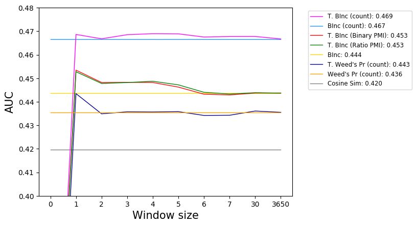
Arsenal-played and lost against-Man United 1-3 (25/01/2019)
    Arsenal-played and beat-Man United 2-0 (10/03/2018)
    Arsenal-played and tied with-Man United 1-1 (30/09/2019)

          Figure 1: Example sentences (left) and their resulting (collapsed) entailment/non-entailment graph (right)

  The contributions of this work are: 1) a model for incorporating relation-level time intervals into an
entailment graph mining procedure, outperforming non-temporal models, and 2) a manually constructed
evaluation dataset of sports domain predicates. To our knowledge this is the first attempt to incorporate
temporal information for learning entailment graphs.

2     Related Work
2.1    Entailment Graphs
Entailment graphs have been constructed for a range of domains, including newswire (Hosseini et al.,
2018), health (Levy et al., 2014), and commonsense (Yu et al., 2020). In order to leverage temporal
information, our work focuses on the news domain, in which each article has a known publication date
and temporal expressions are commonly used.
   A range of node representations have been explored, including Open-IE propositions (Levy et al.,
2014), typed predicates (Berant et al., 2011; Hosseini et al., 2018), and eventualities (Yu et al., 2020). In
this work we use typed predicates, leveraging the second level in the FIGER hierarchy (Ling and Weld,
2012), to enable a close examination of events that take place between two sports teams.
   Whether predicates in the graph entail each other may be determined using a variety of similarity
measures. These are inspired by the Distributional Inclusion Hypothesis, which states that a predicate
p entails another predicate q if for any context in which p can be used, q may be used in its place
(Dagan et al., 1999; Geffet and Dagan, 2005). They include the symmetric Lin’s similarity measure (Lin,
1998), the directional Weeds’ precision and recall measures (Weeds and Weir, 2003), and the Balanced
Inclusion score (BInc) (Szpektor and Dagan, 2008). BInc, the geometric mean of Lin’s similarity and
Weed’s precision, combines the desirable behaviors of symmetric and directional measures. We adapt
and examine each of these similarity measures using our evaluation dataset.
   Alternatively, Hosseini et al. (2019) performed link prediction on the set of relation triples extracted
from the text, and showed improvements over BInc by augmenting the data with additional predicted
triples. We consider this link prediction model to be beyond the scope of this work.

2.2    Evaluating Entailment Graphs
The construction of entailment datasets has been framed as a number of manual annotation tasks includ-
ing image captioning (Bowman et al., 2015) and question answering (Levy and Dagan, 2016).
   The dataset creation method used by Levy and Dagan (2016) aims to address the bias towards real
world knowledge. They ask human annotators to mark possible answers to questions as True/False
(entailment/non-entailment), with entities in the answer replaced using tokens representing their type
(e.g. London becomes city). The method also aims to address the bias of other datasets such as Zeichner’s
dataset (Zeichner et al., 2012) and the SherLIic dataset (Schmitt and Schütze, 2019), in which candidate
entailments were automatically pre-selected for manual annotation according to a similarity measure.
Entailments that exist, but are not captured by these similarity measures will therefore be excluded.
   There has been very little work on the specific problem of evaluating entailment of a temporal nature.
The FraCas test suite (Cooper et al., 1996) contains a small section of which only a few examples are

                                                             61
entailments between predicates. The TEA dataset (Kober et al., 2019) consists of pairs of sentences in
which temporally ordered predicates have varying tense and aspect, such as is visiting → has arrived,
but does not include non-entailments that can be learned through the temporal separation of events (such
as the outcome predicates win and lose that we are interested in). Since there is no dataset to evaluate
this phenomenon, we construct our own (Section 4.1). Our method for dataset construction is similar to
that of Berant et al. (2011). They manually annotated all edges in 10 typed entailment graphs, resulting
in 3,427 edges (entailments) and 35,585 non-edges (non-entailments).
3 Method
3.1 Relation Extraction
We use a pipeline based on a Combinatory Categorial Grammar (CCG, (Steedman, 2000)) parser to
extract binary relations with time intervals. These relations are used to construct typed entailment graphs
using the unsupervised method of Hosseini et al. (2018), adapted to compare only pairs of relations
that are temporally near each other. We extract binary relations of the form arg1-predicate-arg2 (e.g.
Arsenal-beat-Man United), following the example of Lewis and Steedman (2013) and Berant et al.
(2015). We use a pipeline approach similar to that described by Hosseini et al. (2018), which allows us
to extract open-domain relations. Relations are extracted from the NewsSpike corpus (Zhang and Weld,
2013) of news articles collected from multiple sources over a period of approximately six weeks.
We traverse dependency graphs generated over the output of the Rotating CCG parser (Stanojević and
Steedman, 2019), starting from verb and preposition nodes, until we reach an argument leaf node. The
traversed nodes are used to form (lemmatised) predicate strings, and arguments are classified as either a
Named Entity (extracted by the CoreNLP Named Entity recogniser), or a general entity (all other nouns
and noun phrases). Predicate strings may include (non-auxiliary) verbs, verb particles, adjectives, and
prepositions. Negation nodes are detected via string match (“not”, “n’t”, and “never”), and are included
in the predicate if there is a path between the negation node and a node in the predicate. We map passive
predicates to active ones. Modifiers such as “managed to” as in the example “Arsenal managed to beat
Man United” are also extracted and included in the predicate. As the modifiers may be rather sparse, we
extract the relation both with and without the modifier.
We extract and resolve time expressions in the document text, using SUTime (Chang and Manning,
2012), available via CoreNLP. If there is a path in the CCG dependency graph between the time expres-
sion and a node in the predicate, the relation is assigned a time interval. Entities are mapped to types
by linking to their Freebase (Bollacker et al., 2008) IDs using AIDA-Light (Nguyen et al., 2014), and
subsequently mapping these IDs to their fine-grained FIGER types (Ling and Weld, 2012).
To restrict the data to the sports domain we filter the set of output relations, accepting only those
involving two entities of the fine-grained FIGER type organization/sports team. This results in a set of
78,439 binary relations extracted from 24,147 articles, of which 14,664 (approximately 19%) have time
intervals derived from SUTime. The sports domain has the advantage that events are similar and should
be easily separable in time, and it provides the straightforward win-lose-tie outcome set. Sports data is
common in NewsSpike, and sports teams have reliable Named Entity linking, making it suitable for an
initial investigation. In the future we will apply this method to other entity type pairs.
3.2 Graph Construction
The input to the graph construction step is the set of typed binary relations paired with their time intervals.
As we focus on events that involve two sports teams, the output is a single organization-organization
graph, rather than the typical set of graphs (one for every pair of types). Note that these graphs con-
tain only locally learned entailments, and that global inference across graphs is not performed. This is
sufficient to demonstrate the benefit of incorporating time intervals.
In the original method for computing local entailment scores, Hosseini et al. (2018) extract a feature
vector for each typed predicate (e.g. play with type pair organization-organization). The entity pairs
from the binary relations (e.g. Arsenal, Man United) are used as the feature types, and the pointwise
62mutual information (PMI) between the predicate and the entity pair is the value. These feature vectors
are then used to compute local similarity scores.
We extend this method to consider the time intervals for each of the binary relations, with the goal of
comparing only those events that are temporally near each other. To achieve this, we filter the counts of
predicate q according to whether each event’s time interval overlaps with any of p’s. In other words, an
event in q is retained if it is close enough to any event in p. We consider new local similarity scores based
on both the filtered counts, and scaled PMI scores.
Algorithm 1 describes the process of filtering counts using time intervals. The process uses a set of
edges E between predicate nodes to store filtered count information. We loop through each entity pair ep
and get the list of predicates that occur with that entity pair (line 4). Then, for each pair of predicates,
we instantiate edgeObjects (line 7) between predicates p and q (in both directions), to store the filtered
count information. We also retrieve p and q’s timeObjects, containing a list of the time intervals at which
the predicate and entity pair co-occurred (lines 8–9). For each pair of time intervals we compute whether
there is an overlap (lines 12–19). The filtered count is the total number of events in predicate p that
temporally overlap with any event in predicate q.
The count is stored in the edgeObject edgep,q . Once all counts have been collected, they are used
to compute the similarity measures. The computation of temporal measures is identical to that of the
non-temporal counterparts, but they use the filtered counts as input instead of the regular counts. Each
edgeObject populates a cell in W, the sparse matrix of all similarity scores between predicates p and
q, as presented by Hosseini et al. (2018). The filtered counts are also used to scale the PMI scores (see
section 4.2).
Consider the following minimal worked example: Two matches between Arsenal and Man United,
one where Arsenal wins (on 10/03/2018), and one where they lose (on 25/01/2019). This initially results
in the following extracted predicates and counts: play (2), win (1), lose (1). After filtering, we add a
count of 1 to both the win → play and lose → play edges, and a count of 0 to the win → lose edge (and
its reverse).
We consider three possible sources of time intervals: 1) the resolved time expressions extracted from
raw text using SUTime, 2) the document creation date (provided as metadata in the NewsSpike corpus),
and 3) a combination of the two – using resolved time expressions where these are available, and backing
off to the document creation date where they are not. The intuition behind using time expressions ex-
tracted from the article text is that these ought to more accurately pinpoint the time interval of the events.
However, as such expressions may be sparse, we also investigate the use of the document creation date,
under the assumption that sports news is likely to be reported very close the day of the event.
We also consider a temporal window to extend the time intervals by N days either side. This would
mitigate the problem of sports events being reported several days after the event, especially when we fall
back to the document creation date. For sports matches we would expect to see a benefit in using a small
window of a few days, and a detrimental effect as that window grows increasingly larger. Specifically,
we expect that larger windows would render temporal information useless, preventing our model from
being able to distinguish between two different matches involving the same pair of teams. Time interval
source and window size are event-specific parameters that we experiment with in Section 5.1.
4 Evaluation
4.1 Dataset Construction
We propose a semi-automatic method to construct a small evaluation dataset based on manually con-
structed paraphrase clusters. We start with a small set of predicates for which we know the entailment
pattern, in our case {win, play, lose and tie}. We restrict the dataset to include only those binary rela-
tions that involve two sports teams, by filtering on the fine-grained FIGER (Ling and Weld, 2012) type
organization/sports team. We then order the predicates by their frequency in the corpus, and manually
select paraphrases of our small set with a count of at least 20 (the 235 most frequent predicates). This
results in four clusters of paraphrases, with sizes of 26, 8, 3 and 5 respectively for win, lose, tie and play.
We then automatically generate entailment pairs (1,312 in total), labelling them according to the pattern
63Algorithm 1 Temporal filtering in local graph computation
1: procedure T EMPORAL F ILTER(entity pairs, predicates)
2: E ← initialiseAllEdgeObjects(predicates) . Initialise set of edges
3: for ep in entity pairs do
4: predicatesep ← getP redicatesF orEntityP air(predicates, ep)
5: for p ← 0 to length(predicatesep ) do
6: for q ← p + 1 to length(predicatesep ) do
7: edgep,q , edgeq,p ← getEdgeObjects(E, p, q)
8: time objectsep,p ← getT imeObjects(ep, p)
9: time objectsep,q ← getT imeObjects(ep, q)
10: overlapp ← initialiseV ectorOf Zeros(length(time objectsep,p ))
11: overlapq ← initialiseV ectorOf Zeros(length(time objectsep,q ))
12: for i ← 0 to length(time objectsep,p ) do
13: for j ← 0 to length(time objectsep,q ) do
14: if compareIntervals(time objectsep,p [i], time objectsep,q [j]) = 1 then
15: overlapp .set(i, 1)
16: overlapq .set(j, 1)
17: end if
18: end for
19: end for
20: edgep,q .addEdgeCounts(sum(overlapp )) . Events in p that temporally overlap with any q
21: edgeq,p .addEdgeCounts(sum(overlapq ))
22: end for
23: E.update(edgep,q , edgeq,p )
24: end for
25: end for
26: return E
27: end procedure
in Table 1, with premises in the rows and hypotheses in the columns.
We include the paraphrase category for completeness, although we are more interested in the effect
of separating temporally disjoint sports match outcomes. The paraphrase category contains predicates
of varying gradation, such as crush suggesting a strong victory or eliminate indicating that a team is
knocked out of a tournament. We wish to avoid specific predicates such as eliminate entailing non-
specific predicates like beat. To avoid this issue we manually annotated the predicates for specificity, and
for the paraphrase entailments subset we only generate pairs for non-specific predicates. More generally,
a set of paraphrase clusters with a total of n predicates yields n2 − n pairs (not taking into account the
paraphrase subsets reduction).1 The dataset of 1,312 entailment pairs is available here.
(b) Examples from the evaluation dataset
(a) 1 = entailment, 0 = non-entailment. Blue = base (en-
tailments, and non-entailments from temporally disjoint out- Category Examples Size
comes), orange = directional non-entailment, green = para- defeat → vs
phrases entailment 1 272
crush → face
win lose tie play beat → fall to
outcome 0 446
win 1 0 0 1 outscore → lose
lose 0 1 0 1 play → win
directional 0 272
tie 0 0 1 1 go against → tie
play 0 0 0 1 top → knock off
paraphrase 1 322
defeat → outplay
Table 1: Entailment pairs evaluation dataset
4.2 Similarity Measures
We compute both symmetric and directional similarity measures to learn entailments, making use of
the temporally filtered counts and PMI scores described in Section 3.2. Specifically, we adapted Lin’s
1
The subtracted term comes from duplicate pairs like defeat-defeat
64similarity measure (Lin, 1998), Weeds’ precision and recall measures (Weeds and Weir, 2003), and BInc
(Szpektor and Dagan, 2008). The adaptations of these measures are:
Temporal count-based measures using the temporally filtered counts: Weeds’ precision, recall, and
similarity (harmonic average of precision and recall); Lin’s similarity; BInc using Weed’s precision and
count-based Lin’s similarity.
Temporal PMI-based measures: As a proxy to computing Conditional PMI between an entity pair,
predicate p, and predicate q, which would be computationally expensive (if not infeasible) given the
existing graph construction framework, we scale the original PMI scores. We apply two strategies: 1)
Ratio: scale the original PMI scores according to the ratio of filtered counts to regular counts, 2) Binary:
use the original PMI score if any of the events in predicate p overlap with any event in predicate q,
otherwise set the score to zero. The following measures use the Ratio and Binary PMI strategies: Weeds’
precision, recall, and similarity; Lin’s similarity; BInc using Weed’s PMI precision and Lin’s similarity.
Temporal hybrid BInc measures: Computed using count-based Weeds’ precision and PMI-based
Lin’s similarity, using the temporally filtered counts. We do this for both Ratio and Binary PMI.
We also ensure that for every temporal measure, its non-temporal counterpart is also included, and we
include cosine similarity as a symmetric baseline. In total, we experiment with 29 similarity measures.
5 Experiments, Results and Analysis
5.1 Experimental Settings
As described in Section 3.1 we extract all possible relations from the NewsSpike corpus and map their
entities to types using the FIGER hierarchy. We construct a typed entailment graph for the organiza-
tion/organization type pair using the subset of these relations where both entities are sports teams. We
compute entailment scores using the set of 29 similarity measures described in Section 4.2. Due to space
constraints we highlight results for eight of these measures: BInc and cosine similarity baselines, and the
best performing temporal measures and their non-temporal counterparts.
We experimented with different values for the event-specific time information source and temporal
window described in Section 3.2. We constructed typed entailment graphs using only time expressions
(timexOnly), only the document creation date (docDateOnly), and using time expressions where avail-
able, otherwise backing off to the document creation date (timexAndDocDate). For each of the time
interval sources, we also applied windows of 1, 2, 3, 4, 5, 6, 7, 30 and 3,650 days, as well as no window.
We used the evaluation dataset described in Section 4.1 and Table 1 to evaluate entailments captured
under each of these experimental settings. We evaluate on three different configurations of the dataset:
Base (entailment 1 and outcome 0), Directional (entailment 1 and directional 0), and All (entailment 1,
outcome 0, directional 0, paraphrase 1). When we introduce parameter tuning in future work, we plan to
assign a development/test split to the dataset.
5.2 Temporal Information Source
See Table 2 for area under the curve (AUC) scores for each of the three temporal information sources, for
a range of temporal (T) and non-temporal similarity measures. To evaluate the similarity measures fairly
we calculate AUC under a recall threshold (a recall of 0.75 is reached by all non-timexOnly measures).
The timexOnly source has the weakest performance, since it has access to a sparser set of time intervals
(with only 19% of relations linked to a time expression in the text). When we focus on the low recall
range (< 0.15), however, we find that the temporal measures outperform the non-temporal ones. This
is especially promising as it highlights the benefit of using the more accurate time intervals resolved
from time expressions in the text; these give temporal measures a larger increase than the document date.
When using only the document creation date (docDateOnly), we find that temporal and non temporal
measures perform similarly. Results for the timexAndDocDate source show that leveraging both time
expression and document time information together leads to the most effective model.
65Similarity measure timexOnly docDateOnly timexAndDocDate
rec < 0.15 rec < 0.75 rec < 0.75 rec < 0.75
T. BInc (Count) 0.111 0.127 0.467 0.469
BInc (Count) 0.106 0.467 0.467 0.467
T. BInc (Ratio PMI) 0.108 0.108 0.446 0.449
T. BInc (Binary PMI) 0.114 0.114 0.446 0.448
BInc 0.093 0.444 0.444 0.444
T. Weed’s Pr (Count) 0.113 0.129 0.436 0.436
Weed’s Pr (Count) 0.087 0.436 0.436 0.436
Cosine Sim 0.100 0.420 0.420 0.420
Table 2: Temporal information source: AUC scores for the base evaluation dataset, and a temporal window size of 4 days
5.3 Temporal Window Size
In Figure 2 we can see that there is a sharp improvement in AUC score for all of the temporally-informed
similarity measures when a window of one day is applied2 . This is likely due to data sparsity and
because sports articles report on the same event on different days. The horizontal lines represent the non-
temporally-informed similarity measures. We can also see that the choice of window size depends on
the similarity measure. For the majority of the temporally-informed similarity measures, a window size
between one and four days works well. For this class of predicates a window size of 4 seems suitable, as
it avoids conflating games that happen on consecutive weekends, while giving some leeway. We discuss
the possibility of using a dynamic window in Section 6.
Figure 2: Effects of window size for the timexAndDocDate temporal information source
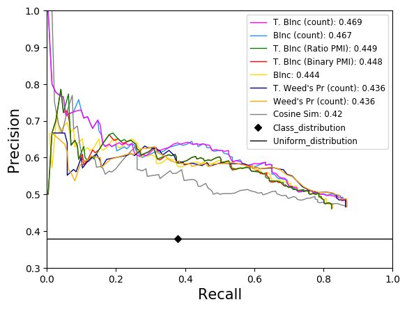
5.4 Comparing Similarity Measures
We can see from Figure 3 that BInc, a state-of-the-art measure for relation entailment, does not perform
well within the temporal setting and is outperformed by a number of the temporal measures. Of those,
T. BInc count sims, the version of BInc that uses the temporally filtered counts, produces the best results
on the base subset of the evaluation dataset. The two temporally informed measures that use scaled PMI
scores (T. Ratio BInc sims and T. Binary BInc sims) also outperform BInc but to a lesser degree. This
may be due to sparsity in the set of binary relations making it difficult to estimate accurate scaled PMI
scores. We hope to alleviate this problem by moving to a larger corpus in future work3 . In more general
terms, for each similarity measure, the temporal version performs better (with the exception of Weed’s
probabilistic precision, for which there is no change).
2
With no window, the temporally informed similarity measures perform poorly (between 0.24 and 0.26)
3
We have already compiled a dataset of 10 years worth of news data from multiple sources
665.5 Performance on Data Subsets
Our main interest is in performance on the base dataset, but for completeness and comparison to previous
work, which tests directionality more, we also evaluated on the all and directional subsets (see Table 3).
To investigate the challenge of directionality in entailment we consider the set of entailments and their
reverse, e.g. play → win (“entailment 1” and “directional 0” in Table 1(b)). We find that in general
the temporal similarity measures still perform strongly. T. Weeds’ precision, the only purely directional
measure in the set, performs comparably to its non-temporal counterpart on the directional subset. The
second best measure is BInc which is unsurprising given that it also captures directionality, and that the
dataset no longer tests temporality.
We also evaluate on the complete dataset (all) which includes paraphrases (“paraphrase 1” in Ta-
ble 1(b)). Here we find that T. Weeds’ precision is again the best measure, closely followed by the
PMI-based T. BInc scores (Binary and Ratio). We expect that the strong performance of T. Weeds’
precision is due to correctly identifying the directional entailments in the dataset, and that the drop in
performance between the directional and all subsets is due to the inclusion of paraphrases, which are
challenging for all measures, but particularly for the Weed’s precision measures which have no symmet-
ric component. BInc also performs reasonably well on this subset, showing that temporally-uninformed
measures remain competitive when multiple phenomena are tested. In general we find that at least one
temporally-informed similarity measure still performs strongly for each of the subsets in the dataset.
Figure 3: Best results on the base evaluation dataset: timexAndDocDate with a temporal window size of 4 days. For calculating
AUC the recall threshold is set to < 0.75 for all similarity measures
5.6 Effects of Using Temporal Information
To see the benefits of including temporal information, we compare the AUC scores for the temporal and
non-temporal similarity measures. We use the timexAndDocDate temporal information source, and a
window size of four days (see Figure 3). The organization-organization graph has 46,899 nodes and be-
tween 7,888,372 and 8,256,182 edges depending on the similarity measure. We can see that the temporal
similarity measure T. BInc count outperforms BInc, the state-of-the-art non-temporal similarity measure
for relation entailment employed by Berant et al. (2011) and Hosseini et al. (2018). We conclude that in-
corporating temporal information is beneficial for accurately predicting entailments and non-entailments
for highly correlated predicates that are part of distinct events.
67Similarity measure Base Dir All
T. BInc (Count) 0.469 0.433 0.433
BInc (Count) 0.467 0.433 0.434
T. BInc (Ratio PMI) 0.449 0.449 0.442
T. BInc (Binary PMI) 0.448 0.449 0.442
BInc 0.444 0.447 0.442
T. Weed’s Pr (Count) 0.436 0.491 0.448
Weed’s Pr (Count) 0.436 0.492 0.447
Cosine Sim 0.420 0.372 0.397
Table 3: AUC scores for different subsets of the evaluation dataset. Temporal information source is timexAndDocDate,
temporal window size is 4 days
6 Discussion and Future Work
The NewsSpike corpus covers a period of approximately six weeks so the outcomes of two matches
between two teams within this period may be fairly similar (as there will have been few changes to the
teams management, players, etc.). In future work we plan to move to a corpus covering a larger time
period, for which we would expect to observe a greater effect. Expanding beyond the sports team domain
would also allow us to study events with longer duration, such as a president holding office, preceded by
their campaign, and election.
Expanding the domain will also give us a collection of local graphs of types beyond just organization-
organization, across which we can then learn globally consistent similarity scores (as in Hosseini et al.
(2018)). We can then also collapse cliques in the graph into paraphrase clusters with a single relation
identifier, which we hope will improve performance, especially on sparser predicates. Our dataset is
perfectly suited to evaluating benefits from this addition due to its origin in paraphrase clusters.
Whilst we can observe a positive effect when using temporal information, the effect is modest. Upon
closer inspection we found that this was due to relatively few events being filtered. An analysis of a
subset of sentences revealed that relations were being extracted spuriously due to various linguistic phe-
nomena. Issues are caused by conditionals (e.g. “if Arsenal win”), modals (“I still expect Arsenal. . . ”),
incorrect future predictions (“Arsenal will win”) and counterfactuals (“had Arsenal won,...”). These types
of predictions appear to be especially common in the sports domain. Another issue arose due to an in-
correct application of passive to active conversion (Arsenal-lost to-Man United from “Man United lost
to Arsenal”) resulting from incorrect verb feature labels in the CCG parses. Finally, SUTime sometimes
provides partial time information which can result in a whole year being used as an interval, creating spu-
rious overlaps4 . Addressing these issues should lead to a larger effect from using temporal information,
because it would reduce overlaps and allow more filtering.
Our algorithm lends itself naturally to mining entailments with a temporal relation such as visit →
arrived. We plan to achieve this by splitting the window into a before and after frame, producing separate
entailment scores for different orderings. We also plan to investigate setting the window dynamically. In
the current setup, events stay relevant for a similar amount of time, but different predicates should allow
comparison for different granularities of time. For example, the window around a person being president
should be larger than a person visiting a location. Initially we might aim to learn a different window size
per predicate (for example by taking into account average predicate duration and granularity). Dynamic
windowing could become particularly valuable with a broader domain.
More generally, our method could incorporate in its filtering any function of the contextualised events
to determine whether their co-occurrence should contribute to an entailment score. Currently a binary
decision is made based on time interval overlap, but one might use features such as (lexical) aspect, tense,
the presence of other entities, etc. Previous work was limited to using the presence of two entities as a
proxy for entailment relevance; with our refinements we could expand to involving not only time but also
4
Focusing only on short time intervals failed to offset the other sources of spurious overlaps
68other features of the contextualised events.
We will also explore the use of other temporal resolution systems and aim to develop more sophisti-
cated ways of linking times to events, which currently only occurs through CCG dependencies. More
time intervals might be propagated using the TempEval (UzZaman et al., 2013) ordering approach or
through other means, for instance by reasoning about tense, Reichenbachian reference time (Reichen-
bach, 1947), or event coreference (within, or across documents).
7 Conclusions
We injected temporal information into the local entailment graph construction method of Hosseini et al.
(2018), with the goal of comparing only those events that are temporally near each other. This is achieved
by filtering the counts of predicate p according to whether its events’ time intervals overlap with the those
of predicate q. We considered a range of new local similarity scores based on both temporally filtered
counts and scaled PMI scores, which we evaluate on a semi-automatically constructed dataset, based on
manually constructed paraphrase clusters.
Our temporal similarity measures outperform their non-temporal counterparts, including BInc, the
state-of-the-art measure for relation entailment. We also show that using a combination of time expres-
sions recovered from the text and the document creation date performed better than using only one of
these sources, and that adding a temporal window around the time intervals of the events is essential. The
performance of the temporal similarity measures over the non-temporal measures is particularly strong
at the low recall range when only time expressions from the text are used. This is especially promising
as it suggests that there is much room for improvement in using more sophisticated temporal resolution
systems and methods for linking times to events.
Acknowledgements
We thank Miloš Stanojević for assistance with the Rotating CCG parser, Nick McKenna and Ian Wood
for helpful discussions, and the reviewers for their valuable feedback. This work was funded by the ERC
H2020 Advanced Fellowship GA 742137 SEMANTAX, a grant from The University of Edinburgh and
Huawei Technologies, and The Alan Turing Institute under EPSRC grant EP/N510129/1.
References
Jonathan Berant, Ido Dagan, and Jacob Goldberger. 2011. Global learning of typed entailment rules. In Proceed-
ings of the 49th Annual Meeting of the Association for Computational Linguistics: Human Language Technolo-
gies, pages 610–619, Portland, Oregon, USA, June. Association for Computational Linguistics.
Jonathan Berant, Noga Alon, Ido Dagan, and Jacob Goldberger. 2015. Efficient global learning of entailment
graphs. Computational Linguistics, 41(2):221–263, June.
Kurt Bollacker, Colin Evans, Praveen Paritosh, Tim Sturge, and Jamie Taylor. 2008. Freebase: A collaboratively
created graph database for structuring human knowledge. In Proceedings of the 2008 ACM SIGMOD Interna-
tional Conference on Management of Data, SIGMOD ’08, page 1247–1250, New York, NY, USA. Association
for Computing Machinery.
Samuel R. Bowman, Gabor Angeli, Christopher Potts, and Christopher D. Manning. 2015. A large annotated
corpus for learning natural language inference. In Proceedings of the 2015 Conference on Empirical Methods
in Natural Language Processing, pages 632–642, Lisbon, Portugal, September. Association for Computational
Linguistics.
Angel X. Chang and Christopher Manning. 2012. SUTime: A library for recognizing and normalizing time
expressions. In Proceedings of the Eighth International Conference on Language Resources and Evaluation
(LREC’12), pages 3735–3740, Istanbul, Turkey, May. European Language Resources Association (ELRA).
Robin Cooper, Dick Crouch, Jan Van Eijck, Chris Fox, Josef Van Genabith, Jan Jaspars, Hans Kamp, David
Milward, Manfred Pinkal, Massimo Poesio, Steve Pulman, Ted Briscoe, Holger Maier, and Karsten Konrad.
1996. Using the framework.
69Ido Dagan, Lillian Lee, and Fernando C. N. Pereira. 1999. Similarity-based models of word cooccurrence proba-
bilities. Machine Learning, 34:43–69.
Maayan Geffet and Ido Dagan. 2005. The distributional inclusion hypotheses and lexical entailment. In Proceed-
ings of the 43rd Annual Meeting of the Association for Computational Linguistics (ACL’05), pages 107–114,
Ann Arbor, Michigan, June. Association for Computational Linguistics.
Mohammad Javad Hosseini, Nathanael Chambers, Siva Reddy, Xavier R. Holt, Shay B. Cohen, Mark Johnson,
and Mark Steedman. 2018. Learning typed entailment graphs with global soft constraints. Transactions of the
Association for Computational Linguistics, 6:703–717.
Mohammad Javad Hosseini, Shay B. Cohen, Mark Johnson, and Mark Steedman. 2019. Duality of link prediction
and entailment graph induction. In Proceedings of the 57th Annual Meeting of the Association for Computa-
tional Linguistics, pages 4736–4746, Florence, Italy, July. Association for Computational Linguistics.
Thomas Kober, Sander Bijl de Vroe, and Mark Steedman. 2019. Temporal and aspectual entailment. In Pro-
ceedings of the 13th International Conference on Computational Semantics - Long Papers, pages 103–119,
Gothenburg, Sweden, May. Association for Computational Linguistics.
Omer Levy and Ido Dagan. 2016. Annotating relation inference in context via question answering. In Proceedings
of the 54th Annual Meeting of the Association for Computational Linguistics (Volume 2: Short Papers), pages
249–255, Berlin, Germany, August. Association for Computational Linguistics.
Omer Levy, Ido Dagan, and Jacob Goldberger. 2014. Focused entailment graphs for open IE propositions. In
Proceedings of the Eighteenth Conference on Computational Natural Language Learning, pages 87–97, Ann
Arbor, Michigan, June. Association for Computational Linguistics.
Mike Lewis and Mark Steedman. 2013. Combined distributional and logical semantics. Transactions of the
Association for Computational Linguistics, 1:179–192.
Dekang Lin. 1998. An information-theoretic definition of similarity. In Proceedings of the Fifteenth International
Conference on Machine Learning, ICML ’98, page 296–304, San Francisco, CA, USA. Morgan Kaufmann
Publishers Inc.
Xiao Ling and Daniel S. Weld. 2012. Fine-grained entity recognition. In Proceedings of the Twenty-Sixth AAAI
Conference on Artificial Intelligence, AAAI’12, page 94–100. AAAI Press.
Dat Ba Nguyen, Johannes Hoffart, Martin Theobald, and Gerhard Weikum. 2014. Aida-light: High-throughput
named-entity disambiguation. Workshop on Linked Data on the Web, 1184:1–10.
Hans Reichenbach. 1947. The tenses of verbs. Time: From Concept to Narrative Construct: a Reader.
Martin Schmitt and Hinrich Schütze. 2019. SherLIiC: A typed event-focused lexical inference benchmark for
evaluating natural language inference. In Proceedings of the 57th Annual Meeting of the Association for Com-
putational Linguistics, pages 902–914, Florence, Italy, July. Association for Computational Linguistics.
Miloš Stanojević and Mark Steedman. 2019. CCG parsing algorithm with incremental tree rotation. In Proceed-
ings of the 2019 Conference of the North American Chapter of the Association for Computational Linguistics:
Human Language Technologies, Volume 1 (Long and Short Papers), pages 228–239, Minneapolis, Minnesota,
June. Association for Computational Linguistics.
Mark Steedman. 2000. The Syntactic Process. MIT Press, Cambridge, MA, USA.
Idan Szpektor and Ido Dagan. 2008. Learning entailment rules for unary templates. In Proceedings of the
22nd International Conference on Computational Linguistics (Coling 2008), pages 849–856, Manchester, UK,
August. Coling 2008 Organizing Committee.
Naushad UzZaman, Hector Llorens, Leon Derczynski, James Allen, Marc Verhagen, and James Pustejovsky. 2013.
Semeval-2013 task 1: Tempeval-3: Evaluating time expressions, events, and temporal relations. In Second
Joint Conference on Lexical and Computational Semantics (* SEM), Volume 2: Proceedings of the Seventh
International Workshop on Semantic Evaluation (SemEval 2013), volume 2, pages 1–9.
Julie Weeds and David Weir. 2003. A general framework for distributional similarity. In Proceedings of the 2003
Conference on Empirical Methods in Natural Language Processing, pages 81–88.
Changlong Yu, Hongming Zhang, Yangqiu Song, Wilfred Ng, and Lifeng Shang. 2020. Enriching large-scale
eventuality knowledge graph with entailment relations. In Automated Knowledge Base Construction.
70Naomi Zeichner, Jonathan Berant, and Ido Dagan. 2012. Crowdsourcing inference-rule evaluation. In Proceed-
ings of the 50th Annual Meeting of the Association for Computational Linguistics (Volume 2: Short Papers),
pages 156–160, Jeju Island, Korea, July. Association for Computational Linguistics.
Congle Zhang and Daniel S Weld. 2013. Harvesting parallel news streams to generate paraphrases of event
relations. In Proceedings of the 2013 Conference on Empirical Methods in Natural Language Processing,
pages 1776–1786.
71You can also read