Improving Viability of Electric Taxis by Taxi Service Strategy Optimization: A Big Data Study of New York City - arXiv
←
→
Page content transcription
If your browser does not render page correctly, please read the page content below
1

                                                          Improving Viability of Electric Taxis by
                                                            Taxi Service Strategy Optimization:
                                                           A Big Data Study of New York City
                                                                                 Chien-Ming Tseng, Sid Chi-Kin Chau and Xue Liu

                                            Abstract—Electrification of transportation is critical for a low-          cation of private vehicles faces many obstacles, such as cost-
arXiv:1709.08463v2 [cs.CY] 18 May 2018

                                         carbon society. In particular, public vehicles (e.g., taxis) provide          effectiveness, availability of home charging infrastructure and
                                         a crucial opportunity for electrification. Despite the benefits of            users’ perception. However, electrification of public vehicles
                                         eco-friendliness and energy efficiency, adoption of electric taxis
                                         faces several obstacles, including constrained driving range, long            (e.g., buses, taxis) would be subject to fewer concerns, with
                                         recharging duration, limited charging stations and low gas price,             even a greater potential impact than that of private vehicles.
                                         all of which impede taxi drivers’ decisions to switch to electric             First, public vehicles are used more frequently, whose elec-
                                         taxis. On the other hand, the popularity of ride-hailing mobile               trification can effectively reduce greenhouse gas emissions.
                                         apps facilitates the computerization and optimization of taxi                 Second, public vehicles are likely to park in common facilities,
                                         service strategies, which can provide computer-assisted decisions
                                         of navigation and roaming for taxi drivers to locate potential                facilitating the installation of charging stations. Third, public
                                         customers. This paper examines the viability of electric taxis with           vehicles generally have shorter life cycles due to frequent
                                         the assistance of taxi service strategy optimization, in comparison           usage, and hence, are more ready to be replaced.
                                         with conventional taxis with internal combustion engines. A big                  Major cities worldwide are introducing plans to phase out
                                         data study is provided using a large dataset of real-world taxi               conventional ICE public vehicles for electric vehicles. For
                                         trips in New York City. Our methodology is to first model the
                                         computerized taxi service strategy by Markov Decision Process                 example, Chinese government has initiated several programs
                                         (MDP), and then obtain the optimized taxi service strategy                    to promote electrification of public vehicles for air pollu-
                                         based on NYC taxi trip dataset. The profitability of electric taxi            tion mitigation [3]. Electric taxi programs were launched in
                                         drivers is studied empirically under various battery capacity and             Shenzhen (in 2010) and Beijing (in 2014) to convert taxis to
                                         charging conditions. Consequently, we shed light on the solutions             electric vehicles, along with the installation of sufficient EV
                                         that can improve viability of electric taxis.
                                                                                                                       parking lots and fast charging points. In these programs, the
                                            Index Terms—Electric vehicles, big data study, taxi service                government also offer subsidies to taxi operators. Singapore
                                         strategy optimization                                                         government plans to roll out a total of 1,000 electric cars to be
                                                                                                                       supported by 2,000 charging points across the city by 2020.
                                                                  I. I NTRODUCTION                                        Nonetheless, unlike buses, taxis are often operated as private
                                                                                                                       businesses. Adoption of electric taxis critically depends on
                                            Taxis are an important part of public transportation system,               the willingness of taxi drivers to switch to electric taxis from
                                         offering both flexibility of private vehicles and shareability                conventional ICE taxis. However, it is not clear whether taxi
                                         of public transportation. In many cities around the world,                    drivers are willing to do so. Despite the initiatives from the
                                         there are usually a large of number of taxis, serving the ad                  governments, there are notable shortcomings of electric taxis:
                                         hoc demands of commuters. Notably, taxis consume a large                        1) Constrained Driving Range: One of the barriers pre-
                                         amount of fuel. For example, there are over 13,000 taxis                            venting wide adoptions of EVs is a shorter driving range.
                                         operating in New York City, which totally travel over 1.46                          With increasing battery capacity, the driving range has
                                         billion kilometers each year1 , and consume over 86 million                         been extended to more than 200 kilometers in production
                                         liters of gasoline. As a result, they emit over 242,900 metric                      EVs such as Chevrolet Bolt. Generally, the driving ranges
                                         tons of CO2 per year2 , which is equivalent to the amount                           of production EVs are sufficient for daily commutes of
                                         of around 25,650 US households’ average annual CO2 emis-                            personal purposes. However, a longer driving range is
                                         sions3 . A viable path toward a low-carbon sustainable society                      normally required by logistic vehicles and taxis (e.g.,
                                         is to promote electrification of transportation, replacing inter-                   more than 300 kilometers). The driving range of high-
                                         nal combustion engine (ICE) vehicles by more environment-                           end Tesla (as in 2017) may suffice to meet the required
                                         friendly and energy-efficient electric vehicles (EVs). Electrifi-                   driving distance, but are too costly for practical taxis.
                                                                                                                         2) Long Recharging Duration: Recharging the battery of
                                           S. C.-K. Chau is with the Australian National University. X. Liu is with
                                         McGill University. (Email: chi-kin.chau@cl.cam.ac.uk, xueliu@cs.mcgill.ca).         EVs can take considerable time. For example, charging
                                           This paper appears in IEEE Transactions on Intelligent Transportation             Nissan Leaf with 30 kwh battery capacity can take up to
                                         Systems (DOI:10.1109/TITS.2018.2839265).                                            4 hours using mode 3 charging, or half an hour using fast
                                           1 According to New York City taxi trip dataset in 2013 [1].
                                           2 Estimated by assuming 67% of New York Yellow taxis as hybrid vehicles           DC charging (without considering queuing delay). Taxis
                                         and 33% as ICE vehicles, as in 2016.                                                traveling long distances are likely to take more than an
                                           3 The average annual CO emission for US household is 9.5 metric tons [2].         hour for recharging between shifts, which is significantly
                                                                   2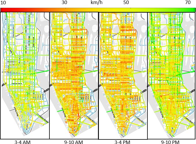
2

      longer than ICE taxis with faster refilling of gasoline.        is determined by a random event of passenger pick-up. The
  3) Limited Charging Stations: Todays, the number of                 uncertainty in taxi service strategy is the pick-up location
      charging stations are few. Also, some of charging stations      and destination of a passenger, which can be estimated by
      are reserved for specific models or brands with propri-         a historical taxi trip dataset.
      etary connectors. The expansion of charging stations is            This MDP model facilitates the optimization of comput-
      hampered by electrical infrastructure in certain regions.       erized taxi service strategies by providing computer-assisted
      As a result, electric taxi drivers always need sufficient       decisions to taxi drivers. Since human taxi service strategies
      reserve battery capacity in order to be able to return to       are inherently inefficient, optimizing computerized taxi service
      certain known charging stations, in case of emergence.          strategies can potentially improve the net revenues of taxi
  4) Low Gas Price: Nowadays, the oil price has come                  drivers, particularly in presence of constraints of driving range
      down considerably from historic heights. This reduces the       and charging stations. Computerized taxi service strategies are
      incentive to adopt EVs, as the gasoline is relatively af-       becoming more feasible, because the increasing adoption of
      fordable, despite cheaper and cleaner electricity sources.      ride-hailing mobile apps, which facilitates the integration of
      Unless carbon tax is introduced to mitigate greenhouse          computerized taxi service strategies in a recommender system
      gas emissions, gasoline ICE vehicles are still perceived        for taxi drivers using real-time data analytics from historical
      as cost-effective by the public in general.                     taxi trip dataset. In this paper, we obtain the optimal policy
   These shortcomings are likely to dissuade taxi drivers from        of MDP that maximizes the revenue of a taxi driver based on
adopting electric taxis. Particularly, it is not easy to operate a    New York City taxi trip dataset, and study the profitability
taxi under the constraints of shorter driving range and limited       of electric taxi drivers under various conditions of battery
charging stations, in comparison with conventional taxis. In          capacity and charging modes.
fact, it has been reported in media that taxi drivers tended
to shun electric taxis. Without taxi drivers’ participation, it is    B. Summary
futile to promote electric taxis. Therefore, it is important to         Our contributions in this paper are summarized as follows:
provide a viability analysis of electric taxis. Such an analysis       1) We formulate an MDP to model computerized electric
can also be used as a basis to determine proper governmental              taxi service strategies, with explicit consideration of con-
subsidies for electric taxis to promote their adoptions.                  straints of EVs, such as battery capacity and locations of
   In this paper, we identify that a key problem of adopting              charging stations.
electric taxis is the ineffective service strategies practiced by      2) We obtain the optimal policy of the MDP based on a big
today’s taxi drivers. In fact, we show that properly optimized            data study using a large dataset of real-world taxi trips
taxi service strategies will not suffer from the shortcomings             in New York City.
of electric vehicles. Therefore, there is a need to provide            3) We study the impact of factors such as battery capacity
an intelligent recommender system to assist taxi drivers to               and charging modes, and locations of charging stations
improve their taxi service strategies, and hence, to increase             on the net revenues of electric taxi drivers.
their willingness to switch to electric taxis. In particular, there    4) We project our study to understand the benefits of a wider
is a popular trend of ride-hailing mobile apps, which facilitates         adoption of electric taxis (up to 1000 taxis).
the computerization and optimization of taxi service strategies,
and provide an opportunity of integrating computer-assisted                                  II. BACKGROUND
optimized decisions of roaming and navigation to taxi drivers.
                                                                      A. Related Work
                                                                         Analyzing taxi trip dataset has been considered by several
A. Modeling Taxi Service Strategy by MDP                              research papers in the subjects of knowledge discovery and
   The net revenue of a taxi driver (i.e., the revenue from taxi      cloud-based intelligent transportation systems [4]. One of
fares minus energy costs) is determined by his/her service            the popular topics is the profit/revenue improvement for taxi
strategy of passenger searching and efficiency of passenger           drivers by developing a recommender system for assisting the
delivery. For example, skilful taxi drivers can identify the          drivers to find passengers more efficiently. The basic idea is to
popular spots for potential passengers, and deliver passengers        identify the good taxi service strategies. Several characteristics
efficiently by choosing faster routes. Note that the service          of taxi service strategies are reported in [5]. Their study
strategies of taxi drivers can be effectively optimized by uti-       shows that searching passengers near the drop-off location
lizing a large historical taxi trip dataset for demand prediction.    of previous passengers results in a higher revenue. They
   To optimize taxi service strategies for electric (or ICE) taxis,   also found that better taxi drivers can deliver the passengers
we first model computerized taxi service strategy by Markov           efficiently by choosing a uncongested route. Furthermore,
Decision Process (MDP). MDP is a general framework for                GPS mobility trace from taxis can be used to predict future
optimizing sequential decision process in the presence of             traffic conditions and optimize the route selections [6]. Also,
uncertainty. In summary, we denote a Markov state as the              community detection has been applied to the mobility trace to
time and location (and possibly battery state) of a taxi, and         reveal potential similar passengers’ travel patterns, as for social
an action as the driver’s decision to travel to the next location     recommendation [7] and improving transportation services [8].
(and possibly recharging operations). At each location, there            Other studies focus on the specific methods for improving
is a probabilistic transition to another location. The transition     the profit/revenue of the taxi drivers. One approach in [9]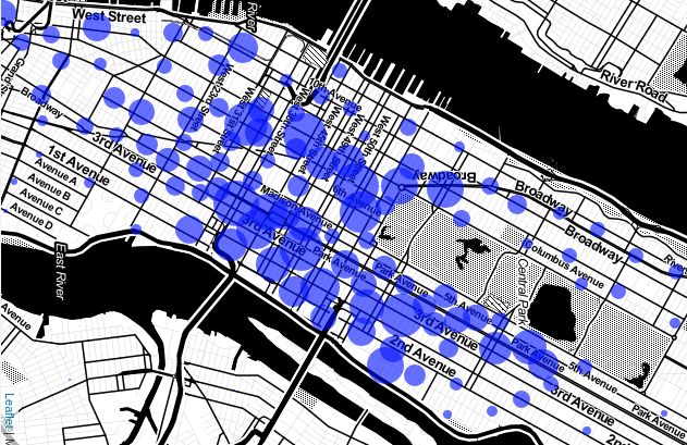
3

shows that experienced taxi drivers usually waits for pas-             displays the pick-up locations on January 16 at 8-9 AM. The
sengers at specific locations, and they are usually aware of           k-means algorithm is employed to cluster the pick-up locations
particular events like train arrivals or ending times of movies.       by 200 clusters. The sizes of circles indicate the number
   Instead of recommending separate pick-up locations, a bet-          of pick-up locations. We observe most of pick-ups occur in
ter approach is to maximize the revenue by selecting a route           Midtown Manhattan. Finally, Fig. 1c displays the locations of
of a sequence of likely pick-up locations at different times.          charging stations in NYC [16] that potentially recharge electric
The top-k profitable driving routes can be computed based on           taxis.
a route network with revenues and pick-up probabilities from
historical taxi trip data in [10]. To select an optimal route                   III. M ARKOV D ECISION P ROCESS M ODEL
with appropriate actions, Markov Decision Process (MDP) is
used to maximize the associated revenue in [11]. The optimal              In this work, we extend the Markov Decision Process
policy of MDP is determined to improve the taxi driver’s               (MDP) framework in [11] to model the computerized service
service strategy. The method of MDP is significantly extended          strategy of an electric taxi. MDP facilitates the formulation
in this paper to consider the constraints of EVs, such as battery      of computerized taxi service strategies, which can be imple-
capacity and locations of charging stations. Our preliminary           mented in a recommender system for taxi drivers. In general, a
study [12] uses a simplified model, whereas this paper presents        MDP comprises of a set of states and a set of possible actions
a more realistic model and a more extensive analysis.                  at each state. Each action transfers the current state to a new
   For EVs, limited driving range is a barrier preventing wide         state with a probability and a reward. The objective is to find
adoption. Therefore, the estimation of driving range for EVs           the optimal actions in the corresponding states that maximize
has been studied in a number of research papers. The driving           the expected total reward.
range of EVs is highly affected by driving speed and motor
efficiency. A black-box model is widely used in the literature         A. States and Actions
to predict the energy consumption of EVs and plug-in hybrid
EVs (PHEVs) [13], [14]. Such a black-box model is used in                First, we explain the states and actions of the MDP in
this paper to estimate the energy consumption of electric taxis.       our setting. A state for an electric taxi is described by three
   There are other studies that investigated the viability of          parameters: current time, current location and battery state, as
deploying electric taxis. For example, the return on investment        explained as follows.
(ROI) for taxi companies transitioning to EVs was studied                 • Current Time: We consider discrete timeslots. One minute
in [15], which considers the mobility trace of yellow cabs                  is used as the interval of a timeslot.
in San Francisco. The prior studies usually assumed that                  • Current Location: We consider the locations represented
electric taxi drivers will adopt the same service strategies as             by the nearest junctions, instead of the absolute locations.
driving a conventional ICE taxi. On the contrary, our study                 A road network is constructed using OpenStreetMap
allows distinctive optimized service strategies for electric taxi           (OSM) junction data. Each pick-up or drop-off location
drivers, taking into account that EVs have different operating              is assigned to the nearest junction in OSM. Let N be the
constraints than conventional ICE vehicles.                                 set of all junctions.
                                                                          • Battery State: We consider discrete levels of state-of-

B. New York City Taxi Trip Dataset                                          charge of battery of the electric taxi. The feasible battery
                                                                            state should be within the range [B, B].
   We describe the taxi trip dataset of New York City (NYC)
                                                                       We denote the location of a taxi at time t by S(t), and the
of 2013 that is used in our study. In the following, we list the
                                                                       battery state by B(t).
attributes of dataset that are used in our study. For each data
record (i.e., a trip), it is composed of following attributes:           The allowable actions at the current junction are the neigh-
                                                                       bors of the junction in the road network, and the recharging
   • Taxi ID (also known as medallion ID)
                                                                       duration, if the electric taxi is subject to recharging at this
   • Trip distance and duration
                                                                       junction. We denote an action from junction i to junction j
   • Times of pick-ups and drop-offs of passengers
                                                                       with recharging duration τ at i by A = (i → j, τ ), where i
   • GPS locations of pick-ups and drop-offs of passengers
                                                                       and j are neighbors in the road network.
We summarize the information of taxi trip dataset in Table I.

     TABLE I: New York City taxi trip dataset in 2013.                 B. State Transition and Objective Function
                       Attribute                           Quantity       The basic idea of the MDP for computerized taxi service
    Num. of medallions (i.e., rights to operate a taxi)      13437     strategy is illustrated in Fig. 2. Assuming the current location
       Annual average traveled distance per taxi          112,600 km
                 Total num. of trips                         175M
                                                                       is i, action A = (i → j, τ ) is taken. The next location will be
            Average num. of trips per day                   450,000    j after recharging for a duration τ at i. When entering junction
                Average trip distance                       4.2 km     j, there is a probability of not picking up any passenger,
                                                                       after which the taxi driver will make another action. On the
  The numbers of taxi trips of NYC dataset on different days           other hand, there is a probability of picking up a passenger,
of 2013 are depicted in Fig. 1a. There are about 450K trips            with a random destination. The taxi driver will decide if the
per day and the average trip distance is around 4.2 km. Fig. 1b        current battery state is sufficient to deliver the passenger to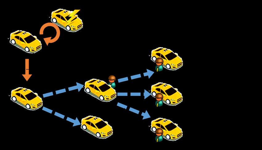
4

                     600000
Average distance Number of taxi trips
                     500000
                     400000
                     300000
                     200000
                                              0   50   100   150     200    250   300   350
                                        5.5
of taxi trips (km)

                                        5.0
                                        4.5
                                        4.0
                                        3.5
                                              0   50   100   150      200   250   300   350
                                                                   Day
                                                                                              (b) Pick-up locations in NYC based on
                                                                                              k-means clustering.                              (c) Charging stations in NYC.
 (a) Num. of trips and average trip distance of NYC
 taxi trip dataset.
                                                                   Fig. 1: Overview of NYC taxi trip dataset and locations of charging stations.

                                                                                                               where t0 , t + Tta (A). The required time of the action Tta (A)
                                                                                                               is computed as follows:
                                                                                                                 1) If recharging duration τ = 0, the taxi directly goes to
                                                                                                                    junction j. The required time of action is given by
                                                                                                                                           Tta (A) = Ttt (i, j)
                                                                                                                 2) If recharging duration τ > 0, before driving to junction
                                                                                                                    j, the taxi first goes to the nearest charging station r(i)
                                                                                                                    to recharge the electric taxi. The required traveling time
                                                                                                                    is Ttt (i, r(i)) to travel to charging station r(i). Then the
                                                                                                                    electric taxi is recharged for τ duration and next goes
                                                                                                                    from charging station r(i) to junction j, whose required
                                                                                                                    traveling time is Ttt+T t (i,r(i))+τ (r(i), j). Thus, the total
                                                                                                                                              t
                                                                                                                    required time of action is given by
 Fig. 2: An illustration of MDP for the computerized service
 strategy of an electric taxi.                                                                                           Tta (A) = Ttt (i, r(i)) + τ + Ttt+Ttt (i,r(i))+τ (r(i), j)
                                                                        Note that if the state-of-charge of battery is insufficient,
 the respective destination, or the trip is discarded. The detailed certain actions are infeasible (e.g., driving to a distant location
 descriptions of MDP are provided in the following.                  to pick up passengers). Therefore, an action needs to consider
    First, we define several parameters for the MDP as follows. the required energy consumption that can be supported by the
         p
     • Pt (i): The probability of successfully picking up a          current battery state. If the current battery state is B(t) = b,
       passenger at junction i at time t.                            after  action A = (i → j, τ ) has been taken, the new battery
         d
     • Pt (i, j): The probability of a passenger commuting from      state  at j will be B(t0 ) = b0 , min{b + τ C − Ete (i, j) −
       junction i to junction j at time t.                           Et (i, r(i)), B}, where C is the charging rate, and t0 , t +
                                                                       e

         a
     • Tt (A): The required time (mins) for executing action A.      Tta (A).
         t
     • Tt (i, j): The required traveling time (mins) from junction      At junction j, there are three possible state transitions:
       i to junction j at time t.                                   (C1)   The taxi successfully picks up a passenger at junction
         e
     • Et (i, j): The required energy consumption (kW) from                j (say, with destination k) and B(t0 ) is sufficient to
       junction i to junction j at time t.                                 deliver the passenger to junction k and then to the
     • Ft (i, j): The net revenue of transporting passengers from          nearest charging station r(k), if necessary. For each k,
       junction i to junction j, which is calculated based on              the probability is Ptp0 (j)Ptd0 (j, k), subject to the constraint
       the fare rule of New York taxi and the respective energy            Ete (j, k) + Ete (k, r(k)) + B ≤ b0 , such that the resultant
       costs. There are various surcharges in different times and          battery state is always larger than the minimal B. Hence,
       days, and hence, the net revenue is time-dependent.                 denote the probability of picking up a passenger by
                                                                                            p
         a
     • Ut (i, j): The energy cost from junction i to j at time t.          probability Pt0 (j)Pts0 (j), where Pts0 (j) is the probability
 Note that some of these parameters (e.g., Ptp (i), Ptd (i, j),            that the destination of passenger is reachable for the taxi
   t           e
 Tt (i, j), Et (i, j)) can be estimated from the taxi trip dataset,        under battery constraint, and is computed by
 which will be discussed in the subsequent section.                                                          X
                                                                                  Pts0 (j) =                                   Ptd0 (j, k)
    Next, we formulate a recurrent equation for describing the
                                                                                              k∈N :Ete (j,k)+Ete (k,r(k))+B≤b0
 MDP, namely, Eqn. (1) (as illustrated in Fig. 3).
    If the current location is S(t) = i, after action A = (i → (C2) The taxi successfully picks up a passenger at junction
 j, τ ) has been taken, the next location will be S(t0 ) = j,              j, but B(t0 ) is insufficient to deliver the passenger to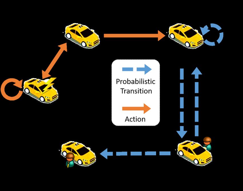
5

                                                          X
    R∗ [t, i, b, A] = 1 − Pt0 (j) +                                              Pt0 (j)Ptd0 (j, k) · R∗ [t0 , j, b0 ]
                           p                                                      p

                                             k∈N :Ete (j,k)+Ete (k,r(k))+B>b0
                                          X                                                                                                             (1)
                                                                Ptp0 (j)Ptd0 (j, k) · Ft0 (j, k) + R∗ t0 +Tj,k,t         0
                                                                                                          t

                         +                                                                                       0 , k, b    − Ete0 (j, k) − Uta (i, j)
                             k∈N :Ete (j,k)+Ete (k,r(k))+B≤b0

      junction k and then to the nearest charging station r(k).
      The total probability of such a case is
                          X
                                         Ptp0 (j)Ptd0 (j, k)
               k∈N :Ete (j,k)+Ete (k,r(k))+B>b0

(C3) The taxi cannot successfully pick up a passenger at
                                               p
      junction j. The probability is 1 − Pt0 (j).
   Note that the probability that the taxi does not deliver any
 passenger (including (C2) and (C3)) is 1 − Ptp0 (j) · Pts0 (j). The
 complement of Pts0 (j), i.e., 1 − Pts0 (j) is given by
                                  X
       1 − Pts0 (j) ,                                Ptd0 (j, k)
                          k∈N :Ete (j,k)+Ete (k,r(k))+B>b0

Hence, we obtain                                                                         Fig. 3: An illustration for the recurrent equation Eqn. (1).
     1−   Ptp0 (j)   · Pts0 (j)
   =1 −   Ptp0 (j)   + Ptp0 (j) · (1 − Pts0 (j))                                         To obtain the optimal policy for the MDP, one can use
                                     X                                                dynamic programming. The dynamic programming algorithm
   =1 −   Ptp0 (j)   +                                     Ptp0 (j)Ptd0 (j, k)
                                                                                      starts from the last timeslot and then works backwards to the
                        k∈N :Ete (j,k)+Ete (k,r(k))+B>b0
                                                                                      beginning timeslot. For example, to solve the optimal policy
   For (C1), the taxi driver will receive a fare of amount                            for a morning shift, the algorithm starts to solve the maximal
Ft0 (j, k), and the next location of the taxi becomes S(t0 +                          expected net revenue at the end of shift, and works backwards.
  t
Tj,k,t 0 ) = k. For (C2) and (C3), the taxi driver will not

receive any fare, and will decide to drive to another location                                IV. M ARKOV D ECISION P ROCESS PARAMETERS
or possibly recharge the taxi.
   The objective of the MDP is to maximize the total expected                           In this section, we estimate several parameters of MDP (e.g.,
                                                                                       p
net revenue. Note that the net revenue of the action is the                           Pt (i), Ptd (i, j), Ttt (i, j), Ete (i, j)) from NYC taxi trip dataset.
received fare minus the energy cost of the action. The expected
net revenue for an action A = (i → j, τ ) at state (t, i, b) is                       A. Driving Speed Network
denoted by R∗ [t, i, b, A], which can be computed recurrently                            First, we construct a driving speed network from the NYC
in Eqn. (1), where                                                                    taxi trip dataset, for the following purposes:
        0            a           0
   • t = t + Tt (A) and b = min{b + τ C, B}.                                            1) To estimate the traveling time from each junction to the
          ∗        0               ∗      0
   • R [t, j, b ] = maxA R [t, j, b , A] is the maximal ex-                                 nearest charging station.
      pected net revenue in state (t, j, b0 ) over all possible                         2) To estimate the energy consumption of a taxi for a trip.
      actions.                                                                        Note that traveling time and driving speed are time-dependent
          a
   • Ut (i, j) is the energy cost, as computed as follows:
                                                                                      parameters, since they are highly affected by traffic condition,
     1) If recharging duration τ = 0, the taxi directly goes to                       which is estimated from historical trip data. For example, the
           junction j. The energy cost is Uta (i, j) = Ete (i, j) · U ,               traveling time between the same pair of junction i and junction
           where U is the unit price, such that U =20 cent/kWh                        j will be higher in office hours and much lower at midnight.
           for electricity and U =2.5 USD$/gallon for gasoline.                          The first step of constructing the driving speed network is to
     2) If recharging duration τ > 0, the taxi goes to the                            determine the driving path of a taxi. Spatialite [17] is used to
           nearest charging station r(i) to recharge the electric                     calculate the shortest path for each pair of pick-up and drop-
           taxi at charging rate C. The energy cost of the action                     off locations. Spatialite utilizes OpenStreetMap (OSM) data.
           is given by                                                                A resulting path comprises a list of edges (i.e., segments)

           Uta (i, j) = Ete (i, r(i))+Ete+Ttt (i,r(i))+τ (r(i), k)+τ ·C ·U            described by two junctions. We then compare the recorded
                                                                                      trip distance in the taxi trip dataset to the computed shortest
  We seek to devise an optimal policy π for the MDP that                              path distance. If the difference is greater than 300 meters,
maximizes the expected net revenue:                                                   the record is discarded since the driver is likely to take other
     π(t, S(t), B(t)) = arg max R∗ t, S(t), B(t), A

                                                     (2)                              route. For each computed path, the segments of a path are
                                         A                                            labeled with the average speed using recorded traveling time
6
and distance. We can obtain the average speed for each taxi trip Denote by λ̄t1 ,t2 the median of idling ratio between time t1
record. Each segment has several average speeds by different and t2 in the distribution. Fig. 5 shows the distribution of idling
trips. We select the highest speed to represent the driving ratios. We observe that the median is 56% for 9-10 AM, but
speed of the segment, since this is usually the speed with only 33% for 3-4 AM due to less traffic.
minimal obstacles. Driving speed networks at different times
are visualized in Fig. 4. We observe there is relatively more B. Passenger Pick-up Probability Ptp (i)
congested traffic in 9 to 10 AM or 4 to 5 PM.
The passenger pick-up probability describes the chance of
a taxi driver can pick up a passenger at junction i at time t.
Following the idea in [11], we use the numbers of taxis and
pick-ups around a particular junction to calculate the pick-up
probability Ptp (i) in τ mins. First, denote the number of pick-
p
ups at junction i from time t to t + τ by Nt:t +τ (i). To estimate
the number of taxis around junction i in τ mins, denote the
number of drop-offs from time t−τ to t+τ within δ kilometers
distance from junction i by Ntd-τ :t+τ (i). Assuming the taxis
are vacant after dropping off the passengers and are roaming
immediately around junction i within δ kilometers in τ mins.
Thus, pick-up probability Ptp (i) can be estimated by
p
p Nt:t +τ (i)
Pt (i) = p (3)
Nt:t+τ (i) + Ntd-τ :t+τ (i)
The suitable parameters τ and δ can be obtained from the
historical taxi trip dataset. For example, τ can be estimated by
Fig. 4: Visualizations of driving speed networks. the average inter-pick-up duration, the time interval between
consecutive pick-ups of a taxi. Using the average driving
Given the driving speed network, we can estimate the speed, δ can be estimated by the reachable distance in the
driving time from the network. We can also estimate the average inter-pick-up duration. Fig. 6a depicts the average
idling time of each trip by subtracting the estimated driving inter-pick-up durations for weekdays and weekends. We ob-
time from the recorded traveling time. The detailed steps for serve that it takes more time to find a passenger at 4 AM
calculating the idling time are described as follows: on weekday and at 7 AM at weekends. Fig. 6b depicts the
1) Average traveling time Ttt (i, j): There may be several respective reachable distance in inter-pick-up duration.
trips start from junction i to junction j. However, their In the following study, we set time-varying τ and δ accord-
traveling times may be slightly different. We average the ing to the average inter-pick-up duration and the respective
traveling time of these trips. reachable distance from taxi trip dataset for each hour.
2) Driving time Ttd (i, j): The shortest path from junction i to
junction j is determined by Spatialite. Then, the driving 20 9
18 Weekday 8 Weekday
time in each segment is computed by its distance and the 16 Weekend 7 Weekend
duration (min)
14
Distance (km)
6
Inter pickup
driving speed from the driving speed network. 12 5
10 4
3) Idling time Tti (i, j): The idling time of a trip is obtained 8
6 3
by subtracting the driving time from the average traveling 4 2
time, Tti (i, j) = Ttt (i, j) − Ttd (i, j) 2 1
00 2 4 6 8 10 12 14 16 18 20 22 24 00 2 4 6 8 10 12 14 16 18 20 22 24
Hour of day Hour of day
1500 0.33 0.56 150 0.7 (a) Inter-pick-up durations for (b) Reachable distances in inter-
Median idling ratioλ̄
λ̄ 9, 10
1200 120 0.6 weekdays and weekends. pick-up durations.
λ̄ 3, 4
900 90
Number
0.5 Fig. 6: Parameters for estimating pick-up probability.
600 60
300 30 0.4
00.0 0.2 0.4 0.6 0.8 1.00 0.3 0 4
d
8 12 16 20 24 C. Passenger Destination Probability Pt (i, j)
Distribution of Idling ratio λ Time of day
The passenger destination probability describes the chance
(a) Distribution of idling ratios for 3-4 (b) Median idling ratios over that a passenger needs to commute from one junction to
AM and 9-10 AM a day.
another junction. This probability is time-dependent, because,
Fig. 5: Hourly distribution of idling ratios and median idling for example, passengers are more likely to commute from
ratio over a day. living places to offices in working hours. One-hour timeslot
is used to estimate passenger destination probability from
To understand traffic conditions, define a metric called the taxi trip dataset. In each timeslot, we obtain the number
T i (i,j)
idling ratio of each source and destination pair by λ , Ttt (i,j) . of trips between each pair of source and destination, and
t7
then is normalized by the total number of trips. Denote the 1) Spatialite is used to find the nearest charging station r(i)
destination probability from junction i to junction j at time for junction i in the road network by the shortest distance.
t by Ptd (i, j). Denote the number of pick-ups at junction 2) The shortest distance is converted into the required driv-
i by Ntp (i), and the number of corresponding drop-offs at ing time based on the driving speed network.
junction j by Ntd (i, j). The passenger destination probability 3) The median idling ratio λ̄ is used to estimate the idling
from junction i to junction x is estimated by time at time t.
4) Given the driving speed network and idling time, the
Ntd (i, j)
Ptd (i, j) = p (4) energy consumption Ete (i, r(i)) is obtained by Eqn. (5).
Nt (i)
F. Taxi Net Revenue Ft (i, j)
D. Energy Consumption Ete (i, j)
The fares are calculated according to the rules for New York
We use a black-box approach to estimate the energy con- taxis. Since there are different kinds of surcharge based on
sumption for EVs, based on the work in [13], [14]. The times and days, the fare is time-dependent, because of various
energy consumption model is based on the average driving surcharges5 . The net revenue of a trip can be calculated by
speed and auxiliary loading. The total energy consumption deducting fuel/electricity cost from the revenue. Therefore, the
can be decomposed into moving energy consumption and net revenue of a trip from junction i to junction j at time t is
auxiliary loading energy consumption, which can be estimated
by multivariate linear models (see [13], [14] for details): Ft (i, j) = FtR (i, j) − Ete (i, j) · U (8)
Ete (i, j) = Etmv (i, j) + Etax (i, j) (5) where FtR (i, j) is the recorded amount of base fare plus the
surcharges from i to j at time t, and U is the unit price.
Etmv (i, j) = β(α1 vt (i, j)2 + α2 vt (i, j) + α3 ) · D(i, j) (6)
Etax (i, j) = `t Ttt (i, j)/60 (7)
G. Charging Rate C
where vt (i, j) is the driving speed between junctions i and j Two types of charging rates are considered in this study:
at time t, obtained from driving speed network. D(i, j) is the mode 3 charging and (direct current) fast charging. Currently,
driving distance between junction i and junction j. mode 3 charging is more common than fast charging. The
The auxiliary loading `t is highly affected by weather charging power of mode 3 charging is 6.6 kW (e.g., for Nissan
temperatures which is time variant. The auxiliary loading Leaf), whereas the charge power of fast charging is 50 kW.
can be estimated from the historic weather temperature and
the average auxiliary loading measurements at particular tem-
V. E VALUATION BASED ON NYC TAXI T RIP DATASET
peratures4 . According to New York historical weather and
suggested power load, the average auxiliary loading is between In this section, we apply the MDP to optimize computerized
1.5 to 1 kW. The parameter β represents aggressiveness factor taxi service strategies and evaluate the improvement in net
to capture the driving behavior. Driver behavior has an impact revenues using NYC taxi trip dataset. We first examine the
on the energy consumption of vehicles, as driving range will be net revenue of conventional ICE taxis and improvement by
significantly decreased by aggressive acceleration and deceler- MDP under a basic setting with complete knowledge of taxi
ation. Mild driving behavior can save up to 30% to 40% energy trip information for one single taxi, which represents the best-
consumption comparing with aggressive driving behavior [19], case scenario. Next, we study a similar setting for electric
[20]. Therefore, we define three classes of driving behaviors: taxis. Then, we relax the basic setting by more realistic
i) mild drivers (β = 0.8), ii) normal drivers (β = 1), and iii) settings: (1) using only historical data as training dataset, (2)
aggressive drivers (β = 1.2). Based on previous work [13], an extension to multiple taxis, and (3) considering different
the parameters of energy consumption model for Nissan Leaf driving behavior.
are set as α1 = 0.1554, α2 = −5.4634, α3 = 189.297.
A. Basic Setting of ICE Taxi
E. Energy Consumption Ete (i, r(i)) Setting: This section presents an evaluation study based on
The electric taxis should arrive at each junction with cer- one-day data of January 9 2013 in the NYC taxi trip dataset.
tain battery state, which can guarantee them to reach the In Sec. V-G, an evaluation using a whole year’s data will be
nearest charging stations. The locations of NYC charging presented. First, we note that the NYC taxi trip dataset has only
station data are obtained from [16]. We consider the charging records of trip distance and duration, and pick-up and drop-off
stations for general EVs. Note that there are other charging information. There is no full mobility data trace of taxis, in
stations requiring memberships, and are not considered in this particular when the taxis are roaming without passengers. It
study. To estimate the minimum required energy consumption 5 The initial charge is $2.50. Plus 50 cents per 1/5 mile or 50 cents per
Ete (i, r(i)) to the nearest charging station r(i) at junction i 60 seconds in slow traffic or when the taxi is stopped. 50-cent MTA State
at time t, the minimum distance between the junction and the Surcharge is required for all trips that end in New York City. Another 30-
cent Improvement Surcharge is required. Daily 50-cent surcharge is required
nearest charging station is obtained as follows: from 8pm to 6am. $1 surcharge is required from 4pm to 8pm on weekdays,
excluding holidays. Toll fees are ignored since the taxi driver will not receive
4 See [18] for an empirical measurement study any revenue from tolls.8
700 224.9 440.3 79.7 155.0 213.2 484.3 79.9 168.4
600 MDP: 0.01% MDP: 0.7% MDP: 0.01% MDP: 0.2%
500 Median Median Median Median
Number
400
300
200
100
00 100 200 300 400 500 0 50 100 150 200 0 100 200 300 400 500 0 50 100 150 200
Estimated net revenues (USD) Delivery distances of passengers (km) Estimated net revenue (USD) Delivery distances of passengers (km)
(a) Estimated net revenues for morn- (b) Delivery distances of passen- (c) Estimated net revenues for (d) Delivery distances of passen-
ing shifts. gers for morning shifts. evening shifts. gers for evening shifts.
Fig. 7: Distributions of estimated net revenues and delivery distances of passengers.
500 8.7 26.8 36.7 500 7.8 30.0 40.3
Median MDP: 2.4% Median MDP: 4.4%
400 Median 400 Median
300 300
Number
Number
200 200
100 100
00 2 4 6 8 10 12 10 15 20 25 30 35 40 45 50 00 2 4 6 8 10 12 10 15 20 25 30 35 40 45 50
Working hour (hr) Hourly net revenue (USD/hr) Working hour (hr) Hourly net revenue (USD/hr)
(a) Working hours for morning (b) Estimated hourly net rev- (c) Working hours for evening (d) Estimated hourly net rev-
shifts. enues for morning shifts. shifts. enues for evening shifts.
Fig. 8: Distributions of working hours and estimated hourly net revenues.
is difficult to estimate the exact total travel distance (i.e., in- shifts. The blue dashed line indicates the median of taxi
cluding roaming and passenger delivery). Hence, we estimate drivers. We observe that 50% drivers earn above USD$223.
a lower bound for the total travel distance by connecting the The red dashed line indicates the expected estimated net
shortest path between a drop-off location and a subsequent revenues when a taxi driver follows the optimal policy of MDP
pick-up location. As such, we obtain an optimistic estimation assuming 12 working hours. This taxi driver is expected to
of net revenue (i.e., revenue minus fuel cost) by the lower earn USD$440. Therefore, optimizing the taxi service strategy
bound of total travel distance. We consider a basic setting, enables a taxi driver to earn at most among the top 0.01%.
such that the optimal policy of MDP is employed in one single Fig. 7b shows the delivery distances of passengers per taxi
taxi, based on complete knowledge of taxi trip information on drivers. More than 50% taxis travel more than 79 kilometers
the same day from the dataset. In Sec. V-D, using historical for passenger delivery. By optimizing taxi service strategy, a
data for prediction and multiple taxis will be presented. taxi driver is expected to travel up to 155 kilometers for pas-
Note that it is challenging to evaluate the exact performance senger delivery. Fig. 7c-7d show the distributions for evening
of modified taxi behavior using historical dataset. For example, shifts. The median net revenue is smaller than that of morning
when a passenger is picked up by a taxi with modified behav- shifts because of shorter working hours (Fig. 8c). Also, we
ior, who was originally picked up by another taxi in the dataset, observe that the median delivery distances of passengers for
it is not clear how original taxi should behave in the evaluation. the evening shift is similar to that of morning shifts.
Therefore, we consider a simple approach of evaluation, such
The computation of expected net revenue of the optimal
that other taxis always follow the recorded trajectories as in
policy of MDP assumes 12 working hours. The distribution
the dataset, no matter picking up the supposed passengers
of working hours for morning shifts is shown in Fig. 8a. We
of the dataset or not. Although this will not attain absolute
observe that most of drivers work less than 12 hours, and
accuracy, this is a simple approach without the knowledge of
the median working hours on the day is 8.7 hours. For a
the disrupted behavior of other taxis in real life. Note that if
normalized comparison, we also study the hourly net revenues,
we only modify the behavior of a small number of taxis, then
instead of net revenues per shifts. The distribution of estimated
this simple approach will give rather accurate evaluation.
hourly net revenues for morning shifts is presented in Fig. 8b.
Also, refueling is not considered for ICE taxis, because ICE
We observe that the hourly net revenue of MDP driver is the
taxi drivers normally fill up the gas tanks between the shifts6 .
top 5% in both shifts. We notice that higher hourly net revenue
Then the MDP model for an ICE taxi is identical to that of
is due to shorter working hour with long trips. Fig. 8c shows
an electric taxi in Sec. III, but without recharging decisions.
that taxi drivers have shorter working hours for evening shifts,
Observations: Based on the NYC taxi trip dataset, Fig. 7a
but their hourly net revenues, because of extra surcharge for
shows the distribution of (optimistically) estimated net rev-
evening shifts.
enues from all the trips (with 11746 taxi drivers) for morning
Ramifications: Optimizing taxi service strategies can sig-
6 Most
NYC taxis operate in two shifts per day. Each normally lasts for 12 nificantly improve the profitability of taxi drivers. Our evalua-
hours. More than 40% of taxi drivers change shifts at around 5 AM or 5 PM.
In this study, we assume that a morning shift is from 5 AM to 5 PM, whereas tion based on a basic setting shows that optimized service strat-
an evening shift is from 5 PM to 5 AM. egy for a conventional ICE taxi can earn at most among the9
ICE Benchmark Fast charging ICE Benchmark Fast charging 70 70
Total energy consumption
Total energy consumption
Mode 3 charging Mode 3 charging Mode 3 charging From charging station
500 500 60 60
475 475 Fast charging Original in battery
Net revenue (USD)
Net revenue (USD)
450 450 50 50
425 425 40 40
(kWh)
(kWh)
400 400 30 30
375 375 20 20
350 350
325 325 10 10
300 30 50 70 300 30 50 70 0 0
Battery capacity (kWh) Battery capacity (kWh) 30 50 70 30 50 70
Battery capacity (kWh) Battery capacity (kWh)
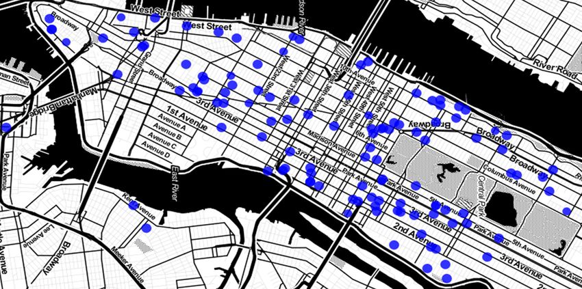
(a) Estimated net revenues of (b) Estimated net revenues of (c) Energy consumptions for morn- (d) Energy consumptions for
electric taxis for morning shifts. electric taxis for evening shifts. ing shifts. evening shifts.
Fig. 9: Estimated net revenues and energy consumptions of electric taxis.
440 ICE benchmark 440 ICE benchmark 440
Use Jan./6 (Sun) Use Jul./14 (Sun)
420 420 420
Net Revenue (USD)
Net Revenue (USD)
Net Revenue (USD)
Use Jan./6 Use Jul./14
400 Use Jan./7 400 (Sun) 400
380 Use Jan./8 380 Use Jul./15 380
360 Use Jan./9 360 Use Jul./16 360
Use Jan./10 Use Jul./17
340 340 Use Jul./18 340
Use Jan./11 Fast charging
320 Use Jan./12 320 Use Jul./19 320
Mode 3 charging
300Mon Tue
300Mon Tue Wed Thu Fri Sat Sun 300Mon Tue Wed Thu Fri Sat Sun Use Jul./20 Wed Thu Fri Sat Sun
(a) Estimated net revenues different dates in (b) Estimated net revenues different dates in July (c) Estimated net revenues using
January as training data with 70 kWh battery as training data with 70 kWh battery capacity. historical data with 30 kWh bat-
capacity. tery capacity.
Fig. 10: Estimated net revenues using historical data for electric taxis.
top 0.1%. Although this represents the best-case evaluation, using optimized service strategies (i.e., USD$426 benchmark),
the subsequent sections will relax to more realistic settings, because electricity cost is cheaper.
and yet still show a considerable advantage. Figs. 9c-9d show the driving distances and energy consump-
tions under different battery capacities. The blue bordered
bar represent the driving distances using fast charging while
B. Basic Setting of Electric Taxi red bordered bars represent those using mode 3 charging.
Setting: In this section, we apply a similar basic evaluation The green portions represent the amount of charging energy
based on the data of January 9 2013 to electric taxis. We received from charging stations, while gray portions represent
employ the energy consumption model of Nissan Leaf [13]. the amount from initial batteries. We observe that the total
In fact, the most determining factor of performance of EVs driving distance is around 242 kilometers without recharging
is battery capacity. Hence, the energy consumption model for morning shifts. At night, the electric taxis are expected
of Nissan Leaf suffices to provide a generic estimation of to drive longer distances because of less traffic. The required
energy consumption of electric taxis. Usually, the EVs will energy consumption without charging for morning shifts is
not allowed to be overly re/discharged to protect the battery. 43 kWh, which can be provided by 50 kWh battery (i.e.,
Therefore, we set the available battery level from 5% to 95% 45 kWh usable capacity) without recharging. For evening
of the capacity. We consider typical settings of battery capacity shifts, the required energy consumption increases to 45.1 kWh.
for EVs (e.g., 30 kWh, 50 kWh, 70 kWh). Each setting can Therefore, electric taxis with 50 kWh battery are then required
affect the recharging decisions and net revenues considerably. to recharge during shifts.
Observations: Figs. 9a-9b show the estimated net revenues Ramifications: Optimizing taxi service strategies for elec-
for electric taxis under different battery capacities. The blue tric taxis can improve the profitability of taxi drivers. But the
bars represent the net revenues using fast charging, while the effect depends on the battery capacity. With more capacity
red bars represent those using mode 3 charging. We observe (e.g., 50 kWh, 70kWh), the taxi driver can earn comparable
that electric taxis equipped with 50 kWh battery can make net revenue with the one of ICE taxi using optimized service
comparable net revenues with traditional ICE taxis using fast strategy. It is because that recharging will incur inefficiency
charging for morning shifts. Note that in general smaller for electric taxis with a low capacity battery.
batteries require more frequent recharging, which can reduce
revenue. EVs with smaller batteries are cheaper. The net C. Using Historical Data for Prediction
revenue gap between using fast charging and mode 3 charging Setting: The previous basic evaluation of net revenues is
is smaller when the battery capacity increases. The estimated based on MDP using the complete knowledge, which requires
net revenue reaches USD$438 when battery capacity is above knowing the pick-up demands and locations in a-priori man-
50 kWh. The net revenue is higher than that of ICE taxis ner. However, complete information is difficult to obtain in10
Driving distance Delivery distance
500 300 425 Mon Tue Wed Thu Fir Sat Sun
1.0 Profit 70 kWh 30 kWh EV 30 kWh EV
450 250
Net revenue (USD)
Net Revenue (USD)
400 fast charging mode 3 charging
0.8
Distance (km)
400 200 375
0.6 350 150 350
Ratio
0.4 300 100 325
0.2 250 50 300
600 800 10000
0.01 2 3 4 5 6 7 8 9 10 200 50 200 400 2750 200 400 600 800 1000 0 200 400 600 800 1000 0 200 400 600 800 1000
Num. of electric taxis in a junction Number of electric taxis Number of electric taxis
(a) Histogram of number of (b) Estimated net revenues for multiple (c) Estimated net revenues for multiple electric taxis over year 2013.
taxis in a junction. electric taxis with 70 kWh battery ca-
pacity.
Fig. 11: Estimated net revenues for multiple electric taxis.
practice. A more practical approach is to use only historical drivers. The junction will become less desirable, when the
data as training dataset for MDP, and then obtain an optimal number of taxis currently present exceeds a certain threshold.
policy as a heuristic for other days. In the following, we use Hence, they would not prefer to go to the junction.
the optimal policy of MDP obtained from 6th January to 12th We first empirically study the distribution of number of taxis
January (i.e., the first week after 1st January) as training data. at all the junctions over time from the dataset. We then set of
Then we employ the policy to all morning shifts in the year limit of the number of taxis at each junction according to the
in the evaluation. mean number of taxis at each junction from the dataset. To
Observations: Fig. 10 shows the estimated net revenue satisfy the constraint, some electric taxis would need to follow
using one-day training data on different days of a week. the second-best decisions in the optimal policy. Each taxi state
We observe that the highest net revenue occurs on Friday is initialized by the junction and the time according to the
while the lowest net revenue occurs on Sunday, because dataset. The state of each taxi is tracked and the passenger
of more passengers on Fridays. The figures also show the pick-up probability Ptp (i) is recomputed using Eqn. (3). We
benchmark for ICE taxis using historical data (i.e., gray band). use the optimal policy based on the data of 6th January.
In particular, Fig. 10a shows the net revenue of 70 kWh battery Observations: Fig. 11a displays the histogram of number
capacity using different dates in January as training data. We of taxis in a junction. We observe that the number of taxis in
observe that the training data from 6th January performs the each junction is less than 7 by 99% of time. We set of limit
best while training data from 8th January performs the worst. of the number of taxis at each junction according to the mean
A taxi driver can receive 7.5% higher net revenue using 6th number of taxis at each junction from the dataset.
January data. Fig. 11b shows the net revenues of different numbers of
Fig. 10c shows the net revenues with the 30 kWh battery electric taxis using the optimal policy of MDP on 9 Jan. We
capacity using training data from 6th January. We observe that observe that the net revenue drops to $USD 350 when 1000
12% higher net revenue can be obtained using fast charging electric taxis use the optimal policy of MDP. The red bar
than using mode 3 charging. Electric taxis with 70 kWh battery indicates the total driving distance of the taxis and blue bar
capacity can obtain 2.8% higher than 30 kWh battery capacity indicates the passenger delivery distance. We observe that the
using fast charging. delivery distance drops but the total driving distance remains
Ramifications: Using historical data for prediction, instead relatively steady. This implies that the increase of roaming
of complete knowledge, will inevitably reduce the effective- distance is due to a lower passenger pick-up probability.
ness. However, this creates a similar effect on ICE taxis Fig. 11c shows the average net revenue of multiple taxis over
that also use historical data. Hence, optimizing taxi service entire year of 2013. We observe that the highest net revenue
strategies for electric taxis using historical data still achieves occurs on Fridays while the lowest occurs on Sundays. We also
comparable net revenues as that of ICE taxis. observe that the net revenue is less affected by the number of
taxis when mode 3 charging is used. This is because that the
electric taxis require frequent recharging, which may result in
D. Multiple Electric Taxis less available taxis, and hence, a higher pick-up probability.
Setting: The optimal policy from MDP has been previously Ramifications: If the optimal policy of MDP is deployed
employed in one single taxi. Next, we employ the optimal up to 1000 electric taxis, then the net revenues will decrease,
policy to multiple taxis. The idea is to allow multiple electric as a result of diminishing advantage of computerized service
taxis adopt the optimal policy from MDP, while ensuring the strategies. These 1000 taxi drivers can still earn as top 1.7%
number of taxis being sent to each location is constrained. among traditional taxi drivers without computerized service
Otherwise, this leads to over-provision of taxis at certain strategies.
locations. This simple constraint allows us to decouple the
individual MDP decisions. Otherwise, considering a large E. Considering Driving Behavior
complex problem will be intractable. In practice, we may Setting: Driving behavior plays an important role in energy
display the potential net revenue of each junction to the taxi consumption of vehicles. Aggressive driving behavior results11
ICE Benchmark Normal ICE Benchmark Normal
70 70
Total Energy Consumption
Total Energy Consumption
Mild Aggressive Mild Aggressive Mild Aggressive From charging station
475 475 60 60
Normal Original in battery
Net revenue (USD)
Net revenue (USD)
450 450 50 50
425 425 40 40
(kWh)
(kWh)
400 400 30 30
375 375
350 350 20 20
325 325 10 10
300 30 50 70 300 30 50 70 0 30 50 70 0 30 50 70
Battery capacity (kWh) Battery capacity (kWh) Battery capacity (kWh) Battery capacity (kWh)
(a) Estimated net revenues of (b) Estimated net revenues of (c) Energy consumption of dif- (d) Energy consumption of dif-
different driving behaviors using different driving behaviors using ferent driving behaviors using ferent driving behaviors using
mode 3 charging. fast charging. mode 3 charging. fast charging.
Fig. 12: Estimated net revenues and energy consumptions of different driving behaviors.
Annual net revenue (USD thousand)
in more energy consumption. Furthermore, higher energy 160
consumption rate induces more frequent recharging of EVs,
which reduces the net revenues of the taxi drivers. We study
three classes of driving behaviors: i) mild drivers (β = 0.8), ii) 140
normal drivers (β = 1), and iii) aggressive drivers (β = 1.2).
Observations: Fig. 12 shows the estimated net revenues of 120
different driving behaviors for morning shifts. Fig. 12a shows
the estimated net revenues of different driving behaviors using
100 ICE ICE ICE EV EV EV
mode 3 charging. Mild drivers can receive 14% higher net rev- $2.5 $3.5 $4.5 70 kWh 30 kWh 30 kWh
enue than aggressive drivers when driving 30 kWh Leaf using USD/G USD/G USD/G fast chg. mode 3 chg.
mode 3 charging. However, the net revenue is less affected
Fig. 13: Annual net revenues under different gas prices.
by different drivers when the battery capacity is sufficiently
large to eliminate recharging during a shift. Fig. 12b shows the
estimated net revenues using fast charging. We observe that the Ramifications: We observe that when the gas price in-
net revenue is also less affected by different driving behaviors creases, ICE taxi becomes a less attractive option since its net
because of shorter recharging duration. Fig. 12 shows the revenue decreases. The net revenue of 70 kWh EV is around
energy consumption of different driving behaviors. We observe 3% higher than ICE taxi when gas price is $2.5 USD/G, while
that aggressive drivers consume around 11 kWh more energy it is around 6.6% higher than ICE taxi when gas price increases
than mild drivers. to $4.5 USD/G.
Ramifications: Although the aggressive drivers consumes
20% more energy which only results in $USD2.2 difference
for morning shifts. The result shows that the driving behavior G. Annual Evaluation of NYC Taxi Trip Dataset
only has a higher impact on the net revenue when the battery
capacity is insufficient to eliminate recharging during a shift. 1) Net Revenue Evaluation:
Setting: We employ the optimal policy from 6th January to
F. Considering Different Gas Prices different numbers of electric taxis and estimate the annual net
revenues. Fig. 15 shows the distribution of annual working
Setting: To complete the study of viability of electric taxis,
hours, we observe that the median annual working hour is
we provide a study of ICE taxis’ net revenue under different
around 1800 hours, but many drivers work more than 4300
gas prices. Note that the current gas price in USA is around
hours, equivalent to working almost 12 hours a day. Therefore,
USD$2.5 per gallon, while the current gas price in China is
we consider taxi drivers working every morning shift (i.e.,
around 7.2 RMB per liter, which is equivalent to $4.5 USD per
4380 working hours) to estimate their net revenues.
gallon. We analyze the outcomes of three different gas prices
(i.e., $2.5 USD/G, $3.5 USD/G, $4.5 USD/G) considering the
1 MDP EV driver 1000 MDP drivers in 30kWh EV
optimal policy of MDP for an ICE taxi. fast charging (.15%)
1 MDP ICE driver 1000 MDP drivers in 30kWh EV
Observations: Fig. 13 compares the annual net revenues of 1000 MDP drivers in 70kWh EV (.07%) mode 3 charging (.4%)
1200
ICE taxi under different gas prices, with that of electric taxis 1000 Median
using different charging options. We observe that the annual 800
Number
net revenue with gas price $2.5 USD/G (i.e., the leftmost bar) 600
400
is slightly higher (about USD$ 4000 higher) than that with 200
gas price $4.5 USD/G. We also observe that the comparable 00 1000 2000 3000 4000 20 40 60 80 100 120 140 160
net revenue can be achieved by 30 kWh EV with fast charging Annual work time (hr) Annual net revenue (USD thousand)
when gas price increases to $4.5 USD/G. However, the annual
net revenue of 30 kWh EV with mode 3 charging is much Fig. 15: Annual working hours and estimated net revenues of
lower (about 14% lower), even when the gas price is high. taxi drivers in 2013.12
220 40
Annual energy consumption
200 140 30 kWh with mode 3 charging 35 30 kWh with mode 3 charging
Annual CO2 emission
consumption (MWh)
180 120 70 kWh 30 70 kWh
(k metric tons)
160 ICE ICE
Daily energy
140 100 25
70kWh EV ICE 80
(BWh)
120 70kWh EV ICE 20
100 30kWh EV 30kWh EV 60 15
80 mode 3 charging mode 3 charging 40 10
60 20
40 5
200 50 100 150 200 250 300 350 0 50 100 150 200 250 300 350 0 50
200 400 600 800 1000 0 50
200 400 600 800 1000
Day of year 2013 Day of year 2013 Number of electric taxis Number of electric taxis
(a) Daily energy consumption of (b) Daily energy consumption (c) Annual energy consumption of (d) Annual CO2 emission of dif-
morning shifts. of night shifts. different numbers of electric taxis. ferent numbers of electric taxis.
Fig. 14: Daily and annual energy consumption and CO2 emission.
Observations: The right figure in Fig. 15 shows the esti- strategy for taxi drivers considering electric taxi operational
mated net revenues of different taxi drivers using the optimal constraints. We evaluate the effectiveness of the optimal policy
policy of MDP. There are some observations: of Markov Decision Process using a big data study of real-
• The case of one electric taxi driver using the optimal world taxi trips in New York City. The optimal policy can
policy of MDP can earn 3% higher than that of one ICE be implemented in an intelligent recommender system for
taxi driver. taxi drivers. This becomes more viable especially due to the
• The average net revenue of case of 1000 electric taxis advent of autonomous vehicles. Our evaluation shows that
with 70 kWh battery is ranked top 0.07% among tradi- computerized service strategy optimization allows electric taxi
tional taxi drivers without computerized service strategy. drivers to earn comparable net revenues as ICE drivers, who
• The average net revenue of case of 1000 electric taxis also employ computerized service strategy optimization, with
with 30 kWh battery using mode 3 charging is ranked top at least 50 kWh battery capacity. Hence, this sheds light on
0.4% among traditional taxi drivers without computerized the viability of electric taxis.
service strategy.
The results shows that the optimal policy of MDP can enable
R EFERENCES
electric taxi drivers to make comparable revenues as traditional
taxi drivers. [1] NYC Taxi & Limousine Commission. (2014) Taxicab Fact Book.
2) Carbon Emission Evaluation: [2] USA Environmental Protection Agency. (2017) Greenhouse Gases
Setting: Besides of net revenues as economic motivation, Equivalences Calculator.
[3] South China Morning Post. (2017) After Hong Kong Failure, China’s
an important benefit is the reduction of carbon emission by BYD Joins Singapore Launch.
switching from ICE taxis to electric taxis. Although electric [4] E. Wilhelm, J. Siegel, S. Mayer, L. Sadamori, S. Dsouza, C.-K. Chau,
taxis do not produce tailpipe emissions, the electricity grid and S. Sarma, “Cloudthink: A scalable secure platform for mirroring
transportation systems in the cloud,” Transport, vol. 30, no. 3, 2015.
to recharge the battery may still produce emissions. In this [5] D. Zhang, L. Sun, B. Li, C. Chen, G. Pan, S. Li, and Z. Wu,
section, we estimate the CO2 emission of electric taxis, as “Understanding Taxi Service Strategies From Taxi GPS Traces,” IEEE
compared with ICE taxis, with computerized service strategy Trans. Intell. Transp. Syst., vol. 16, pp. 123–135, 2015.
[6] S. Liu, Y. Yue, and R. Krishnan, “Non-Myopic Adaptive Route Planning
optimization. The CO2 emission factors of electricity and in Uncertain Congestion Environments,” IEEE Trans. Knowledge and
gasoline are obtained from eGrid of Long Island [2]: Data Engineering, vol. 27, pp. 2438 – 2451, 2015.
• Emission factor of electricity: 0.7007 kg/kWh [7] S. Liu and S. Wang, “Trajectory Community Discovery and Recommen-
dation by Multi-Source Diffusion Modeling,” IEEE Trans. Knowledge
• Emission factor of gasoline: 2.348 kg/liter
and Data Engineering, vol. 29, pp. 898–911, 2017.
Observations: We consider taxis working in all shifts. [8] J. Zhao, Q. Qu, F. Zhang, C. Xu, and S. Liu, “Spatio-Temporal Analysis
Fig. 14a shows the daily energy consumption of 1000 taxis of Passenger Travel Patterns in Massive Smart Card Data,” IEEE Trans.
Intell. Transp. Syst., vol. 18, pp. 3135–3146, 2017.
for morning shifts, while Fig. 14b shows the daily energy [9] J. Yuan, Y. Zheng, L. Zhang, X. Xie, and G. Sun, “Where to Find My
consumption for night shifts. We use miles per gallon gasoline Next Passenger?” in ACM Int. Conf. Ubiquitous Computing (UbiComp),
equivalent to convert the consumed gasoline to kWh (i.e., 1 2011.
[10] M. Qu, H. Zhu, J. Liu, G. Liu, and H. Xiong, “A Cost-effective
gallon of gasoline equals to 33.7 kWh). Fig. 14c shows the Recommender System for Taxi Drivers,” in ACM Int. Conf. Knowledge
annual energy consumption of different numbers of electric Discovery and Data Mining (SIGKDD), 2014.
taxis. We observe that ICE taxis consume around 4 times more [11] H. Rong, X. Zhou, C. Yang, Z. Shafiq, and A. Liu, “The Rich and the
Poor: A Markov Decision Process Approach to Optimizing Taxi Driver
energy than electric taxis. Fig. 14d shows the corresponding Revenue Efficiency,” in ACM Int. Conf. Information and Knowledge
CO2 emissions of different numbers of electric taxis. We Management (CIKM), 2016.
observe that up to 15 thousand metric tons CO2 (equal to 1560 [12] C.-M. Tseng and C.-K. Chau, “Viability Analysis of Electric Taxis Using
New York City Dataset ,” in ACM Workshop on Electric Vehicle Systems,
home’s energy use for one year) can be saved by replacing Data and Applications (EVSys), 2017.
1000 ICE taxis by electric taxis. [13] ——, “Personalized Prediction of Vehicle Energy Consumption based
on Participatory Sensing,” IEEE Trans. Intell. Transp. Syst., vol. 18,
VI. C ONCLUSION no. 11, pp. 3103–3113, 2017.
[14] C.-K. Chau, K. Elbassioni, and C.-M. Tseng, “Drive Mode Optimization
In this paper, we employ Markov Decision Process to and Path Planning for Plug-in Hybrid Electric Vehicles,” IEEE Trans.
model computerized taxi service strategy and optimize the Intell. Transp. Syst., vol. 18, no. 12, pp. 3421–3432, 2017.You can also read