Accelerating deployment of offshore wind energy alter wind climate and reduce future power generation potentials - Nature
←
→
Page content transcription
If your browser does not render page correctly, please read the page content below
www.nature.com/scientificreports
OPEN Accelerating deployment
of offshore wind energy alter wind
climate and reduce future power
generation potentials
Naveed Akhtar*, Beate Geyer, Burkhardt Rockel, Philipp S. Sommer & Corinna Schrum
The European Union has set ambitious CO2 reduction targets, stimulating renewable energy
production and accelerating deployment of offshore wind energy in northern European waters,
mainly the North Sea. With increasing size and clustering, offshore wind farms (OWFs) wake effects,
which alter wind conditions and decrease the power generation efficiency of wind farms downwind
become more important. We use a high-resolution regional climate model with implemented wind
farm parameterizations to explore offshore wind energy production limits in the North Sea. We
simulate near future wind farm scenarios considering existing and planned OWFs in the North Sea
and assess power generation losses and wind variations due to wind farm wake. The annual mean
wind speed deficit within a wind farm can reach 2–2.5 ms−1 depending on the wind farm geometry.
The mean deficit, which decreases with distance, can extend 35–40 km downwind during prevailing
southwesterly winds. Wind speed deficits are highest during spring (mainly March–April) and lowest
during November–December. The large-size of wind farms and their proximity affect not only the
performance of its downwind turbines but also that of neighboring downwind farms, reducing the
capacity factor by 20% or more, which increases energy production costs and economic losses. We
conclude that wind energy can be a limited resource in the North Sea. The limits and potentials for
optimization need to be considered in climate mitigation strategies and cross-national optimization of
offshore energy production plans are inevitable.
The increasing demand for carbon–neutral energy production has fostered the rapidly increasing deployment of
offshore wind farms (OWFs). The construction of OWFs is generally 1.5–2 times more expensive than onshore
wind farms1. Additionally, their maintenance/repair, power network, and obtaining observational data for optimi-
zation are more challenging and c ostlier2. Although OWFs are more expensive in construction and maintenance
than onshore wind farms, these costs are offset to some extent by the higher capacity factor (CF) of OWFs due to
the strength of offshore wind resources3. About 10 km off the coast, sea surface winds are generally 25% higher
than onshore winds. These high offshore wind resources can be utilized 2–3 times longer to generate electricity
than onshore wind farms in the same period of time4,5. Europe’s total installed OWF capacity reached 22 GW in
2019; of that capacity, 77% is installed in the North S ea6. As part of the ambitious plans of the EU to reach climate
neutrality a significant increase to 450 GW total offshore wind energy capacity is intended by 2 0507. About 47%
(212 GW) of these will be installed in the North Sea at an annual consenting rate of 8.8 GW per year during the
2020s8. This implies that the North Sea forms one of the worldwide hotspots of OWF development. Figure 1
shows the planning status of OWFs in the North Sea by 2 0199. These massive developments are motivated by
the strong and reliable wind resources in the North Sea at shallow water depths.
Wind farms are usually clustered around transmission lines to minimize deployment and operating costs.
Hence, in addition to the quality of wind resources also the transmission lines determine whether a location is
optimal for a wind farm. Despite the considerable availability of wind resources, evidence suggests that wake
effects, which manifest as a downwind reduction in wind speed, can undermine the potential of cost-efficient
wind energy production10–12. The efficiency limits that can arise from clustering and the overall regional satura-
tion might limit the offshore wind energy production. These important questions at regional and longer times
scales remain yet unassessed and need detailed scientific analysis for an efficient climate mitigation strategy.
Institute of Coastal Systems‑Analysis and Modeling, Helmholtz-Zentrum Hereon, Geesthacht, Germany. *email:
naveed.akhtar@hereon.de
Scientific Reports | (2021) 11:11826 | https://doi.org/10.1038/s41598-021-91283-3 1
Vol.:(0123456789)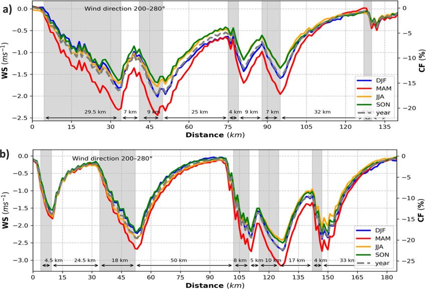
www.nature.com/scientificreports/
Figure 1. Distribution of OWFs in the North Sea (4c Offshore. https://www.4coffshore.com/windfarms/, 2019).
Colors indicate the planning status of the OWFs by 2019. This map was created by Ulrike Kleeberg with ArcGIS
Pro 10.7 (ESRI Inc. ArcGIS Pro 10.7, 2019).
Additionally, in order to develop the OWFs efficiently and accurately, a comprehensive evaluation of the wind
resources is required.
Wind turbines extract kinetic energy (KE) from the atmosphere and convert part of that energy into electric
power. The remaining part of the energy is converted into turbulent kinetic energy (TKE); that generates wakes
(downwind wind speed deficits)13–17. Airborne observations show that TKE is significantly increasing (factor of
10–20) above the wind f arms17. These observations also show that wind farm wakes can extend up to 50–70 km
under stable atmospheric conditions18. These wakes further impact the efficiency of downwind wind farms
through changes in the temperature and turbulence in the boundary layer19. At a given wind speed, colder and
denser air masses provide more energy than warmer and lighter air masses. Moreover, atmospheric turbulence
additionally reduces the energy output and increases the load on wind farm structures and equipment19. Obser-
vational evidence shows that wakes can increase the temperature by 0.5 °C and humidity by 0.5 g per kilogram at
hub height, even as far as 60 km downwind of wind farms20. Case studies related to wake dynamics have largely
been limited to single wind turbines21,22 and/or individual wind farms23–26. Only a few studies have analyzed the
wake effects caused by neighboring wind f arms11,25,27. In a recent s tudy11, the authors highlighted the economic
losses suffered by onshore downwind wind farms due to the wake effects of upwind wind farms. Estimates of the
wake effects on power production and environmental changes have been limited to short timescales (on the order
of a few days or to a specific year28) and only one or two wind farms. The aforementioned studies emphasize the
need to better understand the physical and economic interactions of large wind farms with complex clustered
layouts (such as those planned in the North Sea) to ensure the efficient utilization of wind energy resources.
Building on process understanding of case studies, we assess for the first time the wake effect on the power
production of both existing and planned large OWFs on a regional scale for the North Sea over a period of
10 years. It allows us to take into account the natural variability in wind climate, as inter-annual variability plays
an important role in wind e nergy29. We perform two high-resolution numerical scenario simulations for a multi-
year simulation period, one considering existing and currently planned OWFs in the North Sea and one for the
undisturbed atmosphere. For the future scenario simulation, we apply a generic wind farm parameterization
considering energy extraction and turbulence effects using a standard wind farm configuration, which we validate
Scientific Reports | (2021) 11:11826 | https://doi.org/10.1038/s41598-021-91283-3 2
Vol:.(1234567890)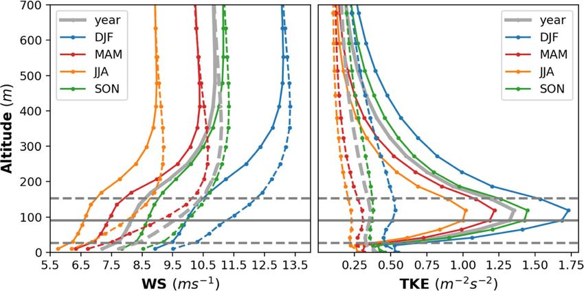
www.nature.com/scientificreports/
Figure 2. Annual and seasonal probability density functions calculated using the hourly (a) wind speed and (b)
wind direction data at FINO1 (6.5875°E and 54.01472°N) at a height of 90 m in the period 2008–2009. Dashed
lines result from measurements, while solid lines are from COSMO-CLM simulation. Gray lines indicate data
for the entire period whereas colors indicate the different seasons as given in the legend.
bservations30 to ensure the realism of the scenario simulation. Mean
against earlier published high-resolution o
wind changes will be analyzed and efficiency loss in offshore energy production will be estimated in terms of the
Capacity Factor (CF) deficiency. Given the ongoing development of OWFs in the North Sea, our study highlights
the urgent need to consider feedbacks between existing and planned OWFs to assess physical and economic
impacts to optimize planning and to assess the limits and environmental impacts of industrial offshore energy
production. To the best of our knowledge, this is the first study to estimate the wind speed deficits due to OWF
production at a basin-wide scale covering a multi-year period and to investigate the effect of these deficits on
the CF of wind farms. Furthermore, in this study, we evaluated the wind farm parameterization for real case
simulations against the observations.
Experimental design
All existing and planned OWFs by 201531 in the North Sea area (see Fig. SI 1, the latest planning status is shown
in Fig. 1) are considered for the scenario simulations. We focus on the Central and Southern North Sea where
OWFs are planned close to each other. The scenario simulations are carried out for a multi-year period from 2008
to 2017, to account for a range of different weather conditions to assess the impact of large-scale OWF devel-
opment on the production potential of wind farms. For the numerical simulations, we use the high-resolution
Consortium for Small-Scale Modeling (COSMO)-CLimate Mode (CLM) regional climate model (RCM)32 both
without and with a wind farm parameterization. An existing wind farm p arameterization15,16,33,34 for a standard
turbine size has been implemented into COSMO-CLM to include the effects of wind farms; these RCM simula-
tions provide us with high-resolution spatiotemporal estimates of the wind speed over wind farm areas. A CF
model35 has been used to assess the average energy production of wind farms based on wind speed. Several
factors can influence the CF, such as the wake effect, turbine efficiency, and offshore d istance36. For the inter-
comparison of scenario simulations, we consider the impact of wakes on the CF, to illustrate the potential impact
of feedbacks between wind farm deployment and regional atmospheric conditions. Hereafter, “CCLM_WF” and
“CCLM” refer to the COSMO-CLM simulations with and without a wind farm parameterization, respectively.
Verification of the simulated wind fields and OWFs wakes
Comparison with the point observations of wind fields. To verify the realism of our scenario simula-
tion, a detailed validation against published data30,37 was performed. The simulated wind characteristics over the
North Sea can be directly evaluated using data from the research p latforms37 FINO1 (6.5875°E, 54.01472°N) and
FINO3 (7.158333°E, 55.195°N) starting in 2004 and 2009, respectively. The high quality of the mast-corrected
measurement data allows for a detailed analysis of both the wind speed and the wind direction. Here we com-
pared the FINO1 and FINO3 measurements with CCLM simulations for the period 2008–2009 and 2009–2014
respectively to avoid the effects of the OWF Alpha Ventus and DanTysk on the mast measurements38. The annual
and seasonal probability density functions (PDFs) derived from hourly values of the wind speed and wind direc-
tion are in good agreement with the FINO1 data (Fig. 2). The annual and seasonal biases, root mean square error
(RMSE), correlation coefficients, and Perkins’ score (PS)39 calculated between the CCLM simulation results
and observations (FINO1 and FINO3) are presented in Tables 1 and 2. Compared with the FINO1 data, the
CCLM winds show small, mostly negative biases of 0.27 ms−1 with simulated wind speeds that are lower than the
observed wind speeds. During the spring and summer season model bias become stronger, along with higher
RMSE values (Table 1). The autumn correlations of 0.87 are slightly higher than those in the other seasons.
The PS of the yearly mean simulated wind speed is 0.95, with the highest values during winter (0.92) and the
Scientific Reports | (2021) 11:11826 | https://doi.org/10.1038/s41598-021-91283-3 3
Vol.:(0123456789)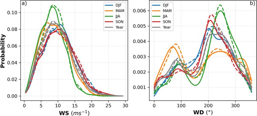
www.nature.com/scientificreports/
Bias RMSE CORR PS
WS (ms−1) WD (°) WS (ms−1) WD (°) WS WD WS WD
Yearly − 0.27 3.07 2.81 70.11 0.79 0.71 0.95 0.92
DFJ − 0.08 1.44 3.41 64.61 0.73 0.71 0.92 0.88
MAM − 0.34 1.21 2.54 76.53 0.82 0.72 0.85 0.77
JJA 0.40 8.08 2.73 72.18 0.72 0.67 0.79 0.80
SON − 0.25 1.40 2.49 65.89 0.87 0.73 0.91 0.87
Table 1. Yearly and seasonal mean wind speed and wind direction bias (CCLM – FINO1), root mean square
error (RMSE), correlation (CORR), and Perkin’s score (PS) of CCLM compared with FINO1 in the period
2008–2009.
Bias RMSE CORR PS
WS (ms−1) WD (°) WS (ms−1) WD (°) WS WD WS WD
Yearly − 0.39 − 6.34 2.59 67.01 0.85 0.75 0.95 0.93
DFJ − 0.54 − 7.95 2.60 55.91 0.87 0.81 0.92 0.88
MAM − 0.40 − 9.12 2.55 70.32 0.84 0.77 0.73 0.80
JJA − 0.30 − 0.45 2.72 79.92 0.75 0.63 0.62 0.78
SON − 0.37 − 7.99 2.50 58.11 0.85 0.79 0.81 0.89
Table 2. Yearly and seasonal mean wind speed and wind direction bias (CCLM – FINO3), root mean square
error (RMSE), correlation (CORR), and Perkin’s score (PS) of CCLM compared with FINO3 in the period
2009–2014.
lowest values during summer (0.79). The simulated CCLM wind direction PDFs are also well represented; the
prevailing southwesterly (200°–280°) wind directions are effectively captured (Fig. 2). On average, the CCLM-
simulated wind directions show a positive bias of 3.07°, a small counterclockwise shift with an RMSE of 70.11°
and a correlation coefficient of 0.71 (Table 1). Again, the simulated summer values show larger deviations from
the observations with a bias of 8.08° and an RMSE of 72.18°; in addition, the correlation coefficient is lower
than those in the other seasons. The simulated wind direction shows the highest PS during winter (0.88) and
the lowest PS during spring (0.77) with a yearly value of 0.92. The simulated wind direction relative to FINO3
shows a negative bias of − 6.34°, an RMSE of 67.01°, a correlation coefficient of 0.75, and a PS of 0.93 (Table 2).
Studies show that the existing wind farms in the North Sea are already affecting the wind field reaching FINO1
and FINO338. A comparison of the wind speed and direction between CCLM_WF and FINO1 shows that the
construction of planned wind farms will further affect their measurements in the future (Fig. SI 2). The annual
and seasonal probability density functions (PDFs) derived from hourly values of the wind speed and wind direc-
tion are also in good agreement with the FINO3 data (Table 2 and Fig. SI 3).
Wake effects in case studies: evaluation of CCLM. For the sake of completeness, CCLM_WF has been
evaluated against airborne campaign data18 to illustrate the ability of CCLM_WF to simulate upwind flow and
the spatial extent of wakes generated by wind farms. Here, we choose two different cases. In the first case, we
evaluate the wake extent of the Amrumbank West wind farm; in the second case, we evaluated the wind speed
deficit over the two Godewind farms. Only operational wind farms at the measurement times are considered in
these simulations. Figure SI 4 shows the model domain and the wind farm locations.
Case 10 September 2016. A detailed comparison is performed for the wakes observed downwind of the
Amrumbank West, Meerwind SüdOst, and Nordsee Ost wind farms with model simulations. The wake was
measured during an aircraft campaign on 10 September 2016 between 0800 to 1100 UTC using five flight legs of
5 km, 15 km, 25 km, 35 km, and 45 km downwind of the Amrumbank West wind farm18,30. Stable atmospheric
conditions and a wake extent of at least 45 km were measured. The installed turbines in Amrumbank West have a
90 m hub height and 120 m rotor diameter12. For this experiment, we employ only those wind farms which were
existing at the time of measurements (see Fig. SI 4).
The simulated spatial extent of the wake agrees well with the measurement. Figure 3 shows the wake extents
simulated in CCLM_WF (interpolated on the aircraft track) and airborne observations (see Fig. SI 5a for a
complete snapshot of the wind speed field simulated in CCLM_WF and its difference from the observation).
Both the observations and the simulations show a wake extending more than 45 km downwind of the wind farm.
The simulation shows that the wake reached down to the Butendiek wind farm, located 50 km downwind of
the Amrumbank West wind farm. However, the simulated wind direction is slightly rotated counterclockwise.
Similar to the width of the wind farms, the wake width is approximately 12 km at the beginning, which expands
and weakens as the distance increases from the generating wind farm. The transect of the simulated and observed
wind speeds through the first flight leg of 5 km downwind of the wind farm shows that the simulated-observed
Scientific Reports | (2021) 11:11826 | https://doi.org/10.1038/s41598-021-91283-3 4
Vol:.(1234567890)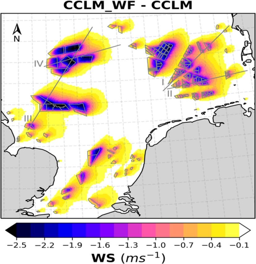
www.nature.com/scientificreports/
Figure 3. Wind speed at 90 m hub height (a) simulated in CCLM_WF and (b) observed by aircraft
measurements. The aircraft track (gray lines) shown here ranged from 0820 to 0924 UTC on 10 September 2016.
The model simulations show the wind speed at 0900 UTC.
differences are smaller inside the wake than outside (Fig. SI 5b). In general, the model slightly underestimates
the wind speed compared to the observations.
Case 14 October 2017. In the chosen case, we evaluate the wind speed at a height of 250 m over Godewind
farms 1 and 2 with aircraft observations. The installed turbines in these wind farms have a 110 m hub height and
153 m diameter18. For this experiment, we employ the wind farm location data as in Fig. SI 4; however, we used
the turbine dimensions as installed in Godewind farms.
Figure 4 shows the wind speeds at 1500 UTC on 14 October 2017 over the Godewind farms simulated in
CCLM_WF (interpolated on the aircraft track) and observed wind speeds (see Fig. SI 6a for a complete snapshot
of the wind speed field simulated in CCLM_WF and its difference from the observation). Stable atmospheric
conditions were observed at the times of the m easurements18. An observed speed-up around the wind farms
is well reproduced in the simulations. The simulated wind speeds agree better with the observations inside the
wake than outside (Fig. SI 6b).
Due to the relatively coarse horizontal resolution of RCMs (1–2 km), the effects of individual wind turbines
(with a rotor span of 120 or 153 m) cannot be fully resolved. Therefore, the simulated wake effects of the wind
turbine can be underestimated, and thus, the wake effects of wind farms can be underestimated. In the present
wind farm p arameterization16, the power produced by the wind turbine depends on the wind speed in the grid
cell at the model level interacting with the rotor. The wind turbine removes momentum from the rotor-interacting
layers to produce the power that leads to wind speed deficits in downwind grid cells.
The evaluation results show that COSMO-CLM with a wind farm parameterization realistically reproduces
the effects of wind farms. The spatiotemporal variability of the wake effects and their impact on the CF of the
wind farms at 90 m hub height are analyzed for the period 2008–2017 in the following sections.
Wake effect on wind speed and turbulent kinetic energy
Our simulations show that the development of massive clustered OWFs significantly impacts the wind climate
and efficiency of renewable energy production on a regional scale. The reduction in the annual mean wind speed
reaches up to 2–2.5 ms−1 during prevailing southwesterly (200°–280°) winds, and that in the seasonal mean
reaches more than 3 ms−1 (see Fig. 5 and Figs. SI 2 and SI 8).
The wind speed in the North Sea exhibits strong spatial and temporal variability. At 90 m hub height, the
wind speed varies seasonally, with a minimum of approximately 7–8.5 ms−1 in summer and a maximum of
10–11.5 ms−1 in winter (Fig. SI 7). The presence of a wind farm impacts the boundary layer flow over the wind
farm and its vicinity by extracting KE from the mean flow and generating TKE. The highest wind speed deficit in
the annual mean is about − 18%, and the increase in TKE is nearly a factor of 4 over the wind farm itself (Fig. 6).
These changes in wind speed and TKE extend vertically to a height of approximately 500 m (about 350 m above
the turbine height). A deficit/raise of about 1 ms−1/0.6 m−2 s−2 in wind speed/TKE extends to a height of approxi-
mately 200 m. The maximum change in wind speed and TKE found in the atmospheric levels between the hub
(90 m) and tip height (153 m) of the wind turbines. The change in the wind speed and TKE above the turbine
height is consistent with the previous studies16,40,41. The wind speed deficits are higher during spring (− 22%)
and summer (− 20.8%) than during the other seasons (see also Fig. SI 8), the reason for which is explained later
in this section. The increase in the TKE is found higher during winter (factor of 3.2) and autumn (factor of 3.8).
The addition TKE source in the wind farm parameterization improves the representation of mixing and wind
speed deficit during stable c onditions17. The change in wind speed and TKE increases the boundary layer h eight16.
Scientific Reports | (2021) 11:11826 | https://doi.org/10.1038/s41598-021-91283-3 5
Vol.:(0123456789)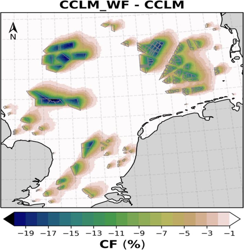
www.nature.com/scientificreports/
Figure 4. Wind speed at a height of 250 m (a) simulated in CCLM_WF and (b) observed by aircraft
measurements. The aircraft track shown here ranged from 1445 to 1500 UTC on 14 October 2017. Arrow
indicates the wind direction. The model simulations show the wind speed at 1500 UTC.
Figure 5. Annual mean wind speed deficits (CCLM_WF – CCLM) outside and inside the wind farms for
the prevailing wind directions of 200°–280° at hub height (90 m) in the period 2008–2017. Numbered gray
lines indicate the transects used for calculations of Fig. 8 and Fig. SI 6 and SI 7. This figure was created with
Matplotlib (Hunter, J. D., Matplotlib: a 2D graphics environment. Computing in Science and Engineering
9, 2007) and Cartopy (Met office, Cartopy: a cartographic python library with a matplotlib interface. Exeter,
Devon, https://scitools.org.uk/cartopy, 2015).
Scientific Reports | (2021) 11:11826 | https://doi.org/10.1038/s41598-021-91283-3 6
Vol:.(1234567890)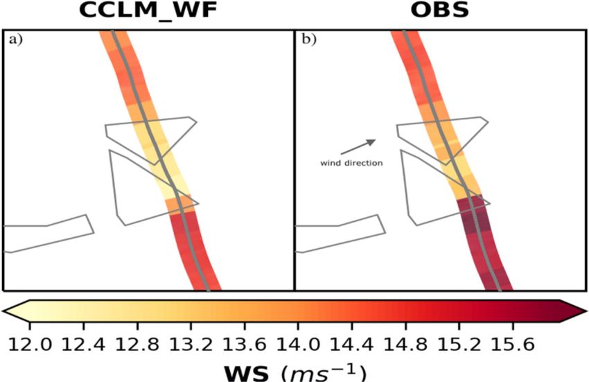
www.nature.com/scientificreports/
Figure 6. Annual and seasonal mean vertical profiles of the wind speed (left) and turbulent kinetic energy
(right) simulated by CCLM (broken dotted lines) and CCLM_WF (solid dotted line) over the wind farm areas
in the period 2008–2017. Solid circles indicate the model levels. The horizontal solid gray line indicates the hub
height (90 m) of the turbine whereas dotted gray lines indicate lower (27 m) and upper (153 m) tip of the rotor.
Wakes, i.e., downwind reductions in wind speed, exhibit significant spatial variability inside and outside wind
farms (Fig. 5). The wind speed deficit inside a wind farm increases with increasing distance from the upstream
edge, reaching a maximum of 2–2.5 ms−1. In an idealized numerical study, a maximum reduction of approxi-
mately 16% in the wind speed and increase in TKE by nearly a factor of 7 was estimated at hub height over a
10 × 10 km wind farm16. Here we used a realistic climate set up to study a scenario with clustered and large-scale
wind farms and found larger mean wind speed deficits of approximately 18–20% of the annual mean wind. In
our case, the increase in the mean TKE within the wind farm is almost a factor of 3 less than that reported (fac-
tor of 7) in the idealized s tudy16. This could be due to the reason that mean values of TKE over a longer period
2008–2017 are shown here.
The wind farm induced boundary layer mixing, air friction, turbulence and weaken stratification effects within
and above the rotor area that reach about 600 m. The maximum differences are found in the layers between
the hub and tip height of the turbine. The reduction in the wind speed extends highest during spring when
the atmospheric conditions are generally stable. The increase in TKE leads to the mixing of more momentum
from aloft15,24. This mechanism is more pronounced during winter and autumn when atmospheric conditions
are generally unstable in the North Sea. The strength of the TKE depends on the difference between the power
coefficient and thrust coefficients which varies with the wind speed.
The wakes forming downwind extend over large distances and influence the wind climate at surrounding
wind farms. The wake extends varies, it depends on wind speed and atmospheric stratification and might extend
up to 70 km downwind11,18,20. On average wakes extend ca 40–45 km downwind (Fig. SI 8).
Implications for the CF
The downwind speed reduction results in a significant decrease in the efficiency of energy production here illus-
trated in terms of the CF. The wake induced decrease in CF up to 22% in the annual mean and up to 26% for the
seasonal mean with the highest values at the downwind edge within the wind farms during southwesterly wind
directions (see Fig. 7 and Figs. SI 4 and SI 5). Outside of the wind farms, these values decrease as the distance
from the wind farms is increasing. A decrease of about 1% has been noted at a distance of 35–40 km in annual
means during southwesterly wind directions. The highest drops are observed for the large wind farms in the
German Bight and the UK’s Dogger Bank for southwesterly wind directions (Fig. 7).
Without the wind farms, the annual mean CF for all wind directions varies spatially in the North Sea from 50
to 62%, with higher values during winter (65–70%) and lower values in summer (37–50%, Fig. SI 9). These values
are strongly reduced in the areas where the large-size wind farms are clustered. The mean wind speed deficits
and CF losses for all wind directions show that the wake effect extends more towards the northeast than in the
other wind directions, indicating the dominance of southwesterly winds (Fig. SI 8 and Fig. SI 10).
A more specific analysis of the implications of large wind farm clusters and extremely large farms for the
efficiency of neighboring farms and clusters in the area of the German Bight and the Dogger Bank (Fig. SI 1)
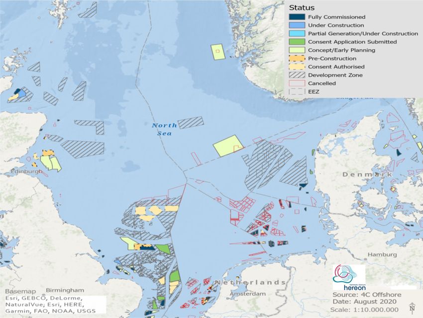
highlights substantial CF losses. Figure 8 shows the annual and seasonal mean wind speed deficits and CF losses
through the wind farms on two of the transects (gray lines I and III) shown in Fig. 5 in the case of prevailing
winds in the German Bight and the UK’s Dogger Bank. The wind farms in both of these areas are large and are
located spatially close to each other. These transects show the strong horizontal influences of the wind farms
together with the reductions in the wind speed and CF. Mean CF and wind speed show characteristic patterns
Scientific Reports | (2021) 11:11826 | https://doi.org/10.1038/s41598-021-91283-3 7
Vol.:(0123456789)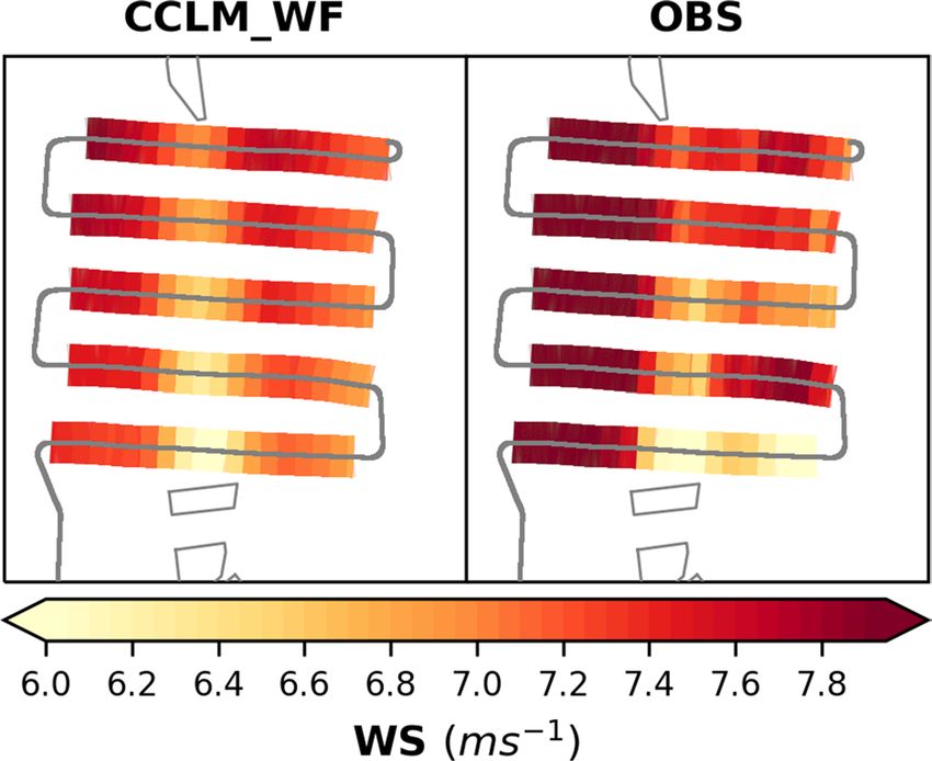
www.nature.com/scientificreports/
Figure 7. Annual mean losses in the capacity factor CF (CCLM_WF – CCLM) out- and inside of the wind
farms (gray lines) for the prevailing wind directions of 200°–280° at hub height (90 m) in the period 2008–2017.
This figure was created with Matplotlib (Hunter, J. D., Matplotlib: a 2D graphics environment. Computing
in Science and Engineering 9, 2007) and Cartopy (Met office, Cartopy: a cartographic python library with a
matplotlib interface. Exeter, Devon, https://scitools.org.uk/cartopy, 2015).
along transects crossing several wind farms (Fig. 8). The wind speed deficit, being higher towards the downwind
wind farm edge, leads to an annual reduction of up to 25% in the CF of downwind wind turbines inside wind
farms; outside these wind farms, the CF losses reach up to 20% depending on the size of the farm and distance
away from it. For example, as shown in Fig. 8a, wind farm 2, which is 7 km from wind farm 1, suffers a mean
wind speed deficit of 1–1.5 ms−1. This reduces the CF of upwind turbines by 10–15% and that of downwind
turbines by 15–20% in wind farm 2. Then, the wakes generated by wind farm 2 extend up to wind farm 3 (25 km
away) with a deficit of 0.5–0.8 ms−1 and CF losses of 5–8%. The wake effect of wind farm 4 reaches up to 30 km.
The wind speed between wind farms 1 and 2 recovers approximately 45% in 5 km. However, the recovery of the
wind speed in the following wind farms is slow due to the accumulated effects. Similarly, as shown in Fig. 8b, the
wake effect reaches approximately 33 km between wind farms 2 and 3 and approximately 28 km beyond wind
farm 5. The wake generated by the wind farm 4 reduces the CF of wind farm 5 (17 km away) up to 12%. Due to
the short distance between wind farms 3 and 4 (about 5 km), wind farm 4 receives about 1.5–2 ms−1 less wind
speed which is equivalent to CF losses of 12–16%, during prevailing southwesterly winds. The transects of lines
II and IV are shown in Fig. SI 11. The most productive wind turbines/farms are those located on the grid-cells
at upwind edge/farms of the wind farms where the wind flow is u ninterrupted25.
The wake effect can substantially influence the economic potential of wind power generation within a cluster,
in large farms, and in neighboring farms located at a distance within the wake. Annual mean wind speed defi-
cits of 1–1.5 ms−1 and CF deficits of wind farms in the vicinity of large downwind clusters are frequent, within
clusters, the reduction is even stronger and amounts up to a seasonal mean wind speed reduction of more than
3 ms−1 or a seasonal CF reduction of up to 25% (Fig. 8). Average wakes extend up to 40 km for the largest wind
farms and clusters.
The highest wind speed deficits occur during the spring season which leads to the highest CF losses in these
seasons. On a monthly timescale, the highest wind speed deficits are simulated in March and April, whereas the
lowest deficits are simulated in November and December (see Fig. SI 12). The seasonal variations in wind speed
deficits are related to the relatively stronger winds (see Fig. SI 12) and weaker stratification42 during the autumn
and winter seasons compared to the spring seasons. During spring, the atmospheric conditions are more stable
than the other seasons which leads to longer w akes18,42–44. It implies that the most productive season is winter
when the wind speed is higher and the stratification not stable.
Discussion and conclusions
The results show that the wind fields simulated by the regional climate model COSMO-CLM are in good agree-
ment with the mast measurement stations FINO1 and FINO3 in the North Sea. It also indicates that the deploy-
ment of large wind farms near the mast measurement stations will affect their measurements. The COSMO-CLM
model with the wind farm parametrization15 simulated the wake generated by the wind farms reasonably well.
Despite the differences in the upwind wind speed, the length and width of the wake were simulated quite well.
Scientific Reports | (2021) 11:11826 | https://doi.org/10.1038/s41598-021-91283-3 8
Vol:.(1234567890)www.nature.com/scientificreports/
Figure 8. (a) Transects of the seasonal (colored, see legend) and yearly mean (dashed gray) wind speed deficits
(left axis; CCLM_WF – CCLM) and capacity factor losses (right axis; CCLM_WF – CCLM) for the prevailing
wind directions of 200°–280° in the period 2008–2017 at hub height (90 m) taken at transect I (German Bight,
Fig. 5) latitude 54.2 latitude 54.2°N–55.6°N and longitude 5.45°E–8.0°E. Gray sectors indicate the wind farm
positions. Arrows and attached numbers give the distances between the edges of the wind farms. (b) As of (a)
but for transect III (Dogger Bank, Fig. 5) latitude 54.4°N–55.8°N and longitude 0.8°E–3.15°E.
Our results show that clusters of large wind farms, such as the farms planned for the near future in the UK’s
Dogger Bank and the German Bight, have the potential to substantially modify the atmospheric dynamics
and lead to local mean wind speed reductions extending as far as more than 40 km downwind from the farm.
Depending on the size of the wind farm, generally, the annual mean wind speed deficit can reach 2–2.5 ms−1
which is equivalent to the power loss of 1–2 kWs45. These results are consistent with the previous s tudies15,46,47.
These authors studied the consequences of wind farms in case studies and short-term simulations. Our results
show that the previously identified effects accumulate and influence the mean wind pattern. We identified a
trade-off in the clustering of offshore wind farms. Clustering supports reduced energy production costs due
to reduced infrastructure investments, but these advantages can be offset by wakes effects and the consequent
reduction of CF. Our results emphasize that wind energy in the North Sea can be considered a limited resource.
With the current plans to install offshore wind energy farms in the North Sea locally resource exploitation limits
are reached. Better planning and optimization of locations are required that consider the development of wind
wakes under realistic multi-year atmospheric conditions.
It is important to note that for our idealized study we used an average size (90 m hub height and 126 m rotor
diameter) of turbines for existing wind farms. The rapidly increasing size and power generation of wind t urbines48
can intensify the wake effects vertically and horizontally. Moreover, wind farm installations in the North Sea are
further accelerating and the here identified limits of power generation will become more important.
Southwesterly winds are predominant in the North Sea49 (Fig. 2 and Fig. SI 3), and wake effects and their
implications for power generation are therefore of particular importance for efficient energy production and
production costs. During prevailing southwesterly winds, the power production of a downwind wind farm on
the northeastern side is generally undermined by the wind farms located upwind.
Under stably stratified atmospheric conditions, weak vertical momentum mixing strengthens the wake
effect11,15,18,20, and observational evidence shows that the wake can extend up to 50–70 km under such atmos-
pheric conditions30. Such individual cases are also well reproduced in the model simulations. These findings
suggest that CF losses can be greater than the mean values shown herein and last longer under stable atmospheric
conditions. Additionally, this study shows the annual and seasonal mean values calculated using hourly values
during the period 2008–2017 to illustrate the mean wake effect on the CF using multi-year weather conditions
Scientific Reports | (2021) 11:11826 | https://doi.org/10.1038/s41598-021-91283-3 9
Vol.:(0123456789)www.nature.com/scientificreports/
under all atmospheric conditions. This shows that the wind speed and CF deficits are highest during spring
(mainly March–April) and lowest during November–December. The proximity of large wind farms affects the
production of downwind wind turbines and wind farms, reducing the CF by more than 20–25%.
Already now, offshore renewable energy production in the North Sea shows substantial impacts on the
atmospheric conditions therein, and these effects will continue to increase in the future. The evidence indicates
that OWFs can impact marine animals and can raise environmental and climate concerns2,50,51. Since wind is
one of the main factors modulating ecosystem productivity and ecosystem structure, OWFs have the potential
to develop into dominant ecosystem drivers and need to be considered for ecosystem management and fisher-
ies assessment. Therefore, an optimization strategy based on both national and international considerations is
required to minimize economic losses and to assess the limits and environmental impacts of industrial offshore
energy production. Furthermore, atmospheric wakes can induce ocean responses by modifying the sea surface
roughness, atmospheric stability, and heat fluxes, and hence have the potential to influence local climate that
requires further i nvestigation32,52,53.
Methods
Numerical model setup. In this study, we employ the regional climate model COSMO-CLM32 with a
wind farm p arameterization15,33,34 to consider the wind farm impacts on local atmospheric dynamics and the
spatial–temporal pattern of wind speed deficits for a near-future wind farm scenario in the North Sea (see Fig.
SI 1). COSMO-CLM uses a horizontal atmospheric grid mesh size of 0.02° (~ 2 km; 396 × 436 grid cells) and
62 vertical levels. In our configuration, COSMO-CLM uses a time step of 12 s with a third-order Runge–Kutta
numerical integration scheme. The physics options include a cloud microphysics scheme, a delta-two-stream
scheme for shortwave and longwave radiation, and a one-dimensional prognostic TKE advection scheme for the
vertical turbulent diffusion p arameterization54. The roughness length over the sea is computed on the basis of
54
the Charnock formula . The initial and lateral boundary conditions for the wind, sea surface temperature and
other meteorological variables are taken from a CoastDat3 simulation29, which provides hourly data at a hori-
zontal resolution of 0.11° (~ 11 km). The CoastDat3 atmospheric simulation was driven by European Centre for
Medium-Range Weather Forecast (ECMWF) ERA-Interim reanalysis data in 6 hourly intervals at a horizontal
resolution of 0.703°55.
To include wind farm effects, a wind farm parameterization for mesoscale numerical weather prediction
models is implemented into COSMO-CLM56. This parameterization represents wind turbines as a momentum
sink for the mean flow that converts KE into electric energy and TKE. The parameterization uses the velocity in
each grid to estimate the average effect of the wind turbines within that grid. In our configuration, we use five
vertical levels within the rotor area. The wind turbine extracts KE from the mean flow of each layer intersecting
the rotor area. The amount of extracted KE depends on the wind speed, thrust, power coefficients, air density,
and the density of the wind turbines in the considered g rid45 (see Fig. SI 13). A fraction of the extracted KE is
converted into electric power by the turbine, whereas the remaining part of KE is converted into TKE. Here, we
use the thrust and power coefficients as a function of wind speed derived from the theoretical National Renewable
Energy Laboratory (NREL) 5 MW reference wind turbine for offshore system d evelopment45. These coefficients
are close to those of real wind turbines, as the NREL 5 MW turbine data were derived from the REPower 5 MW
offshore wind turbine. The wind turbine is hallmarked by a cut-in wind speed of 3 ms−1, a rated power speed of
12 ms−1, and a cut-out speed of 25 ms−1. In this study, we used the 90 m hub height and a 126 m rotor diameter
with a rated power of 5.3 MW. The chosen turbine size falls within the range of existing wind farms by 2017
(Table SI 3). For a more detailed description of the wind farm parameterization and its implementation, we refer
the readers to the previous s tudies15,33,34.
Capacity factor (CF). Because of the high variability of wind, low, medium, and high wind speeds alternate
frequently, and wind turbines cannot operate continuously at the rated power. Therefore, the CF is commonly
used to calculate the average energy production of a wind turbine. In turn, the CF is used for the economic
assessment of a project, optimum turbine site matching, and the ranking of potential sites35. Several generic
models are available in the literature to represent the ascending segment of the power curve between the cut-
in and rated speeds (Fig. SI 13) independent of the power coefficients, which are unique to every turbine and
difficult to generalize. These generic models use the cut-in, rated, and cut-out speeds to estimate the ascending
segment of the power curve without information on the turbine output. We use a polynomial generic model35
to estimate the CF using a Weibull probability density function based on hourly wind speed values and three
speeds, namely, the cut-in (3 ms−1), rated (12 ms−1), and cut-out (25 ms−1), of the performance curve shown in
Fig. SI 13.
Data availability
The model COSMO-CLM_WF and COSMO-CLM datasets supporting the results can be downloaded via CERA-
DKRZ57,58 and the COSMO-CLM namelists are available from the authors upon request. The COSMO-CLM
simulations employ the community-wide publicly available (http://www.clm-community.eu) COSMO-CLM
code. In situ airborne observational data were accessed via P ANGAEA30 and the FINO data were obtained via
https://www.fino-offshore.de/en/ and http://fino.bsh.de.
Received: 31 January 2021; Accepted: 24 May 2021
Scientific Reports | (2021) 11:11826 | https://doi.org/10.1038/s41598-021-91283-3 10
Vol:.(1234567890)www.nature.com/scientificreports/
References
1. Zheng, C. W., Li, C. Y., Pan, J., Liu, M. Y. & Xia, L. L. An overview of global ocean wind energy resource evaluations. Renew. Sustain.
Energy Rev. 53, 1240–1251 (2016).
2. Leung, D. Y. C. & Yang, Y. Wind energy development and its environmental impact: A review. Renew. Sustain. Energy Rev. 16,
1031e9 (2012).
3. Junfeng, L., Pengfei, S. & Hu, G. China Wind Power Outlook 2010 (2010).
4. Tambke, J., Lange, M., Focken, U., Wolff, J. O. & Bye, J. A. T. Forecasting offshore wind speeds above the North Sea. Wind Energy
8, 3–16 (2005).
5. Wang, J., Qin, S., Jin, S. & Wu, J. Estimation methods review and analysis of offshore extreme wind speeds and wind energy
resources. Renew. Sustain. Energy Rev. 42, 313–322 (2015).
6. WindEurope. Offshore wind in Europe: Key trends and statistics 2019 (2019).
7. The European Green Deal. Communication from the commission to the European parliament, the European council, the council,
the European economic and social committee and the committee of the regions (2019).
8. WindEurope. Our Energy Our Future: How offshore wind will help Europe go carbon-neutral (2019).
9. 4c Offshore. https://www.4coffshore.com/windfarms/. (2019).
10. Hasager, C. B. et al. Wind farm wake: The 2016 Horns Rev photo case. Energies 10, 317 (2017).
11. Lundquist, J. K., DuVivier, K. K., Kaffine, D. & Tomaszewski, J. M. Costs and consequences of wind turbine wake effects arising
from uncoordinated wind energy development. Nat. Energy 4, 26–34 (2019).
12. Siedersleben, S. K. et al. Evaluation of a wind farm parametrization for mesoscale atmospheric flow models with aircraft measure-
ments. Meteorol. Z. 27, 401–415 (2018).
13. Rhodes, M. E. & Lundquist, J. K. The effect of wind-turbine wakes on summertime US midwest atmospheric wind profiles as
observed with ground-based Doppler Lidar. Bound.-Layer Meteorol. 149, 85–103 (2013).
14. Djath, B., Schulz-Stellenfleth, J. & Cañadillas, B. Impact of atmospheric stability on X-band and C-band synthetic aperture radar
imagery of offshore windpark wakes. J. Renew. Sustain. Energy 10, 043301 (2018).
15. Fitch, A. C., Olson, J. B. & Lundquist, J. K. Parameterization of wind farms in climate models. J. Clim. 26, 6439–6458 (2013).
16. Fitch, A. C. et al. Local and mesoscale impacts of wind farms as parameterized in a mesoscale NWP model. Mon. Weather Rev.
140, 3017–3038 (2012).
17. Siedersleben, S. K. et al. Turbulent kinetic energy over large offshore wind farms observed and simulated by the mesoscale model
WRF (3.8.1). Geosci. Model Dev. 13, 249–268 (2020).
18. Platis, A. et al. First in situ evidence of wakes in the far field behind offshore wind farms. Sci. Rep. 8, 1–10 (2018).
19. Irena. Renewable energy technologies: Cost analysis series. Green Energy Technol. 1 (2012).
20. Siedersleben, S. K. et al. Micrometeorological impacts of offshore wind farms as seen in observations and simulations. Environ.
Res. Lett. 13, 124012 (2018).
21. Smalikho, I. N. et al. Lidar investigation of atmosphere effect on a wind turbine wake. J. Atmos. Ocean. Technol. 30, 2554–2570
(2013).
22. Churchfield, M. J., Lee, S., Michalakes, J. & Moriarty, P. J. A numerical study of the effects of atmospheric and wake turbulence on
wind turbine dynamics. J. Turbul. 13, 1–32 (2012).
23. Aitken, M. L., Kosović, B., Mirocha, J. D. & Lundquist, J. K. Large eddy simulation of wind turbine wake dynamics in the stable
boundary layer using the Weather Research and Forecasting Model. J. Renew. Sustain. Energy 6, 033137 (2014).
24. Calaf, M., Meneveau, C. & Meyers, J. Large eddy simulation study of fully developed wind-turbine array boundary layers. Phys.
Fluids 22, 015110 (2010).
25. Nygaard, N. G. Wakes in very large wind farms and the effect of neighbouring wind farms. J. Phys. Conf. Ser. 524, 012162 (2014).
26. Nygaard, N. G. & Christian Newcombe, A. Wake behind an offshore wind farm observed with dual-Doppler radars. J. Phys. Conf.
Ser. 1037, 032020 (2018).
27. Nygaard, N. G. & Hansen, S. D. Wake effects between two neighbouring wind farms. J. Phys. Conf. Ser. 753, 032020 (2016).
28. Badger, J. et al. Making the most of offshore wind: Re-evaluating the potential of offshore wind in the German North Sea. Study
commissioned by Agora Energiewende and Agora Verkehrswende, 1–84 (2020).
29. Geyer, B., Weisse, R., Bisling, P. & Winterfeldt, J. Climatology of North Sea wind energy derived from a model hindcast for
1958–2012. J. Wind Eng. Ind. Aerodyn. 147, 18–29 (2015).
30. Bärfuss, K. et al. In-situ airborne measurements of atmospheric and sea surface parameters related to offshore wind parks in the
German Bight. PANGAEA https://doi.org/10.1594/PANGAEA.902845 (2019).
31. EWEA. The European offshore wind industry key 2015 trends and statistics. … Documents/Publications/Reports/Statistics/ … 31
(2015). https://doi.org/10.1109/CCA.1997.627749.
32. Rockel, B., Will, A. & Hense, A. The regional climate model COSMO-CLM (CCLM). Meteorol. Z. 17, 347–348 (2008).
33. Chatterjee, F., Allaerts, D., Blahak, U., Meyers, J. & van Lipzig, N. P. M. Evaluation of a wind-farm parametrization in a regional
climate model using large eddy simulations. Q. J. R. Meteorol. Soc. 142, 3152–3161 (2016).
34. Blahak, U., Goretzki, B. & Meis, J. A simple parameterization of drag forces induced by large wind farms for numerical weather
prediction models. European Wind Energy Conference and Exhibition 2010, EWEC 2010 6, 4577–4585 (2010).
35. Albadi, M. H. & El-Saadany, E. F. Optimum turbine-site matching. Energy 35, 3593–3602 (2010).
36. Dean, N. Performance factors. Nat. Energy 5, 5 (2020).
37. Leiding, T. et al. Standardisierung und vergleichende Analyse der meteorologischen FINO-Messdaten (FINO123) (2016).
38. Westerhellweg, A., Cañadillas, B., Kinder, F. & Neumann, T. Wake measurements at alpha ventus—Dependency on stability and
turbulence intensity. J. Phys. Conf. Ser. 555, 012106 (2014).
39. Perkins, S. E., Pitman, A. J., Holbrook, N. J. & McAneney, J. Evaluation of the AR4 climate models’ simulated daily maximum
temperature, minimum temperature, and precipitation over Australia using probability density functions. J. Clim. 20, 4356–4376
(2007).
40. Lu, H. & Porté-Agel, F. Large-eddy simulation of a very large wind farm in a stable atmospheric boundary layer. Phys. Fluids 23,
065101 (2011).
41. Chamorro, L. P. & Porté-Agel, F. A wind-tunnel investigation of wind-turbine wakes: Boundary-Layer turbulence effects. Bound.
Layer Meteorol. 132, 129–149 (2009).
42. Djath, B. & Schulz-Stellenfleth, J. Wind speed deficits downstream offshore wind parks—A new automised estimation technique
based on satellite synthetic aperture radar data. Meteorol. Z. 28, 499–515 (2019).
43. Emeis, S. A simple analytical wind park model considering atmospheric stability. Wind Energy 13, 459–469 (2010).
44. Christiansen, M. B. & Hasager, C. B. Wake effects of large offshore wind farms identified from satellite SAR. Remote Sens. Environ.
98, 251–268 (2005).
45. Jonkman, J., Butterfield, S., Musial, W. & Scott, G. Definition of a 5-MW reference wind turbine for offshore system development.
Contract https://doi.org/10.1002/ajmg.10175 (2009).
46. Abkar, M. & Porté-Agel, F. Influence of atmospheric stability on wind-turbine wakes: A large-eddy simulation study. Phys. Fluids
27, 035104 (2015).
47. Allaerts, D. Large-eddy simulation of wind farms in conventionally neutral and stable atmospheric boundary layers (2016).
Scientific Reports | (2021) 11:11826 | https://doi.org/10.1038/s41598-021-91283-3 11
Vol.:(0123456789)www.nature.com/scientificreports/
48. IEA. Offshore Wind Outlook 2019. World Energy Outlook https://doi.org/10.1787/caf32f3b-en (2019).
49. Siegismund, F. & Schrum, C. Decadal changes in the wind forcing over the North Sea. Clim. Res. 18, 39–45 (2001).
50. Saidur, R., Rahim, N. A., Islam, M. R. & Solangi, K. H. Environmental impact of wind energy. Renew. Sustain. Energy Rev. 15,
2423–2430 (2011).
51. Tabassum, A., Premalatha, M., Abbasi, T. & Abbasi, S. A. Wind energy: Increasing deployment, rising environmental concerns.
Renew. Sustain. Energy Rev. 31, 270–288 (2014).
52. Boettcher, M., Hoffmann, P., Lenhart, H. J., Heinke Schlunzen, K. & Schoetter, R. Influence of large offshore wind farms on North
German climate. Meteorol. Z. 24, 465–480 (2015).
53. Platis, A. et al. Long-range modifications of the wind field by offshore wind parks—Results of the project WIPAFF. Meteorol. Z.
https://doi.org/10.1127/metz/2020/1023 (2020).
54. Doms, G., Schättler, U. & Baldauf, M. A Description of the Nonhydrostatic Regional COSMO Model. DWD COSMO V5.4. http://
www.cosmo-model.org (2011).
55. Dee, D. P. et al. The ERA-Interim reanalysis: Configuration and performance of the data assimilation system. Q. J. R. Meteorol.
Soc. 137, 553–597 (2011).
56. Akhtar, N. & Chatterjee, F. Wind farm parametrization in COSMO5.0_clm15 (2020) doi:https://doi.org/10.35089/WDCC/WindF
armPCOSMO5.0clm15.
57. Akhtar, N. coastDat-3_COSMO-CLM_HR_WF. World Data Center for Climate (WDCC) at DKRZ. http://cera-www.dkrz.de/
WDCC/ui/Compact.jsp?acronym=DKRZ_LTA_302_ds00001 (2020).
58. Akhtar, N. coastDat-3_COSMO-CLM_HR. World Data Center for Climate (WDCC) at DKRZ. http://cera-www.dkrz.de/WDCC/
ui/Compact.jsp?acronym=DKRZ_LTA_302_ds00002 (2020).
Acknowledgements
The study is initiated and funded by the Initiative and Networking Fund of the Helmholtz Association through
the project “Advanced Earth System Modelling Capacity (ESM)”. The authors would like to acknowledge the
German Climate Computing Center (DKRZ) for providing computational resources, the Federal Ministry for
Economic Affairs and Energy (BMWi) and the Federal Agency for Shipping and Sea for the FINO data, and
Wind Park Far Field (WIPAFF) project for providing first in situ airborne atmospheric observational data of
the offshore wind farms. The authors also acknowledge F. Chatterjee for helping with the implementation of
the wind farm parameterization in COSMO-CLM. The authors thank Johannes Schulz-Stellenfleth for fruitful
discussion and suggestions and Ulrike Kleeberg for contributing Fig. 1. We thank the CLM Community for their
assistance and collaboration.
Author contributions
N.A. and B.R. implemented the wind farm parameterization in COSMO-CLM. N.A. designed the atmospheric
simulations. B.G. provided the forcing data. N.A. and P.S. analyzed the data. B.G. wrote the FINO validation
section. C.S. and B.R. initiated and supervised the work. N.A. wrote the original draft. All authors contributed
to writing, reviewing, and editing the manuscript.
Funding
Open Access funding enabled and organized by Projekt DEAL.
Competing interests
The authors declare no competing interests.
Additional information
Supplementary Information The online version contains supplementary material available at https://doi.org/
10.1038/s41598-021-91283-3.
Correspondence and requests for materials should be addressed to N.A.
Reprints and permissions information is available at www.nature.com/reprints.
Publisher’s note Springer Nature remains neutral with regard to jurisdictional claims in published maps and
institutional affiliations.
Open Access This article is licensed under a Creative Commons Attribution 4.0 International
License, which permits use, sharing, adaptation, distribution and reproduction in any medium or
format, as long as you give appropriate credit to the original author(s) and the source, provide a link to the
Creative Commons licence, and indicate if changes were made. The images or other third party material in this
article are included in the article’s Creative Commons licence, unless indicated otherwise in a credit line to the
material. If material is not included in the article’s Creative Commons licence and your intended use is not
permitted by statutory regulation or exceeds the permitted use, you will need to obtain permission directly from
the copyright holder. To view a copy of this licence, visit http://creativecommons.org/licenses/by/4.0/.
© The Author(s) 2021
Scientific Reports | (2021) 11:11826 | https://doi.org/10.1038/s41598-021-91283-3 12
Vol:.(1234567890)You can also read