Multiobjective Route Selection Based on LASSO Regression: When Will the Suez Canal Lose Its Importance? - Hindawi.com

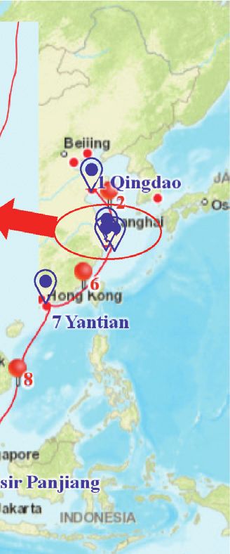
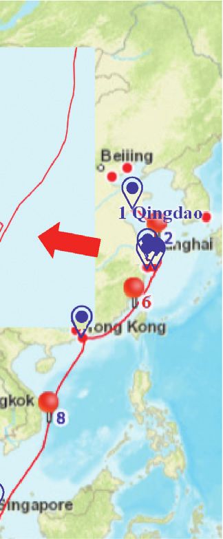
Hindawi
Mathematical Problems in Engineering
Volume 2021, Article ID 6613332, 18 pages
https://doi.org/10.1155/2021/6613332

Research Article
Multiobjective Route Selection Based on LASSO Regression: When
Will the Suez Canal Lose Its Importance?

 Jingmiao Zhou ,1,2 Yuzhe Zhao ,2 and Jiayan Liang 2

 1
 Business School, Dalian University of Foreign Languages, Dalian 116044, China
 2
 Collaborative Innovation Center for Transport Studies, Dalian Maritime University, Dalian 116026, China

 Correspondence should be addressed to Yuzhe Zhao; zhaoyuzhe@dlmu.edu.cn

 Received 13 December 2020; Revised 21 January 2021; Accepted 24 January 2021; Published 19 February 2021

 Academic Editor: Mohammad Yazdi

 Copyright © 2021 Jingmiao Zhou et al. This is an open access article distributed under the Creative Commons Attribution License,
 which permits unrestricted use, distribution, and reproduction in any medium, provided the original work is properly cited.
 With coronavirus disease 2019 reshaping the global shipping market, many ships in the Europe-Asia trades that need to sail
 through the Suez Canal begun to detour via the much longer route, the Cape of Good Hope. In order to explain and predict the
 route choice, this paper employs the least absolute shrinkage and selection operator regression to estimate fuel consumption based
 on the automatic identification system and ocean dataset and designed a multiobjective particle swarm optimization to find Pareto
 optimal solutions that minimize the total voyage cost and total voyage time. After that, the weighted sum method was introduced
 to deal with the route selection. Finally, a case study was conducted on the real data from CMA CGM, a leading worldwide
 shipping company, and four scenarios of fuel prices and charter rates were built and analyzed. The results show that the detour
 around the Cape of Good Hope is preferred only in the scenario of low fuel price and low charter. In addition, the paper suggests
 that the authority of Suez Canal should cut down the canal toll according to our result to win back the ships because we have
 verified that offering a discount on the canal roll is effective.

1. Introduction Canal slashed the transit charge. Apparently, bypassing the
 Suez Canal is driven by external factors like fuel price,
Despite bleak prospects of worldwide market amid the charter rate, and canal transit charge.
coronavirus disease 2019 (COVID-19) pandemic, shipping The additional fuel and charter costs of switching to the
remains the backbone of the global economy [1]. However, longer route are negligible, owing to the drop of fuel prices
shipping companies must reconsider their decision-making and charter rates. More importantly, the growing costs can
of ship operations in order to survive the crisis. Suddenly, be largely offset by the benefits of avoiding the expensive
Europe-Asia sailing via the Cape of Good Hope rather than canal transit charge. It is reported that Maersk shells out
the shorter route via the Suez Canal looks like an attractive approximately 350,000 USD per ship for transiting through
option. As shown in Figure 1 [2], since the end of March the Suez Canal [4]. Under the combined effects of external
2020, at least 32 such sailings took place via the Cape of factors, the detour around the Cape of Good Hope offers
Good Hope. Many ships operated by the three major shipping companies an effective measure to minimize total
shipping alliances, 2M, Ocean Alliance, and THE Alliance, voyage cost.
have all chosen the longer route. In practice, however, the minimal cost is not the only
 Sailing around the Cape of Good Hope, more than 3,000 object in the decision-making of ship operations. The detour
nautical miles and at least 5 days longer than transiting via the longer route inevitably increases the total voyage
through the Suez Canal, may seem to be a strange move. But time, which will lower the service level and may annoy
the preference of this sailing option is not unprecedented. shippers. In fact, some shippers are weighing up whether to
When fuel price nosedived in late 2015, many ships sailing stop booking slots from shipping companies making the
from the US east coast to Asia did the same until the Suez detour [5]. To maintain market share, shipping companies

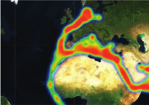
2 Mathematical Problems in Engineering

 (2) Some cutting-edge big data techniques and opti-
 mization methods were applied in combination to
 solve the problem. Specifically, the data preparation,
 training LASSO regression model, multiobjective
 particle swarm optimization (MOPSO) algorithm,
 and WS method were integrated into a novel opti-
 mization framework of sailing speed and sailing
 Suez canal route.
 (3) Four scenarios reflecting the fluctuation of shipping
 market conditions were proposed and analyzed for
 the ship detouring problem. For each scenario, the
 Cape of good hope
 paper also calculated the suggested Suez Canal toll
 Route March April May (mid) that is able to win back the ships detouring around
 Asia-Europe (westbound) 1 7 0 the Cape of Good Hope.
 Europe-Asia (eastbound) 0 7 8
 US EastCost-Asia (eastbound) 0 7 7 The remainder of this paper is organized as follows:
 Section 2 makes a thorough review of the related literature;
Figure 1: Number of containerships switched to the route via the Section 3 establishes a LASSO regression model to estimate
Cape of Good Hope. Note: the data are collected from BIFA [2]; the
 fuel consumption, introduces a multiobjective optimization
heat map is from [3].
 model, describes the solving algorithm MOPSO, and in-
 troduces the WS method; Section 4 presents and analyzes the
must work to improve the service level, i.e., minimizing the optimization results through a case study; and Section 5 puts
total voyage time. Hence, the decision of whether to detour is forward the conclusions.
a multiobjective problem aimed at trading off minimal total
voyage cost against minimal total voyage time.
 Considering the growing popularity of detouring around 2. Literature Review
the Cape of Good Hope, this paper aims to disclose how
external factors influence the decision of whether to detour. Ship operations decision-making mainly includes fleet
To clarify the mechanism of influence, the main obstacle lies management, ship scheduling, route planning, and speed
in the difficulty in precisely estimating the total voyage cost. setting. Christiansen et al. [8] summarized the studies on
For instance, it is very difficult to estimate fuel consumption, ship scheduling and route planning. Mansouri et al. [9]
which is impacted by various factors, such as sailing speed, provide a survey of existing research on sustainable decision-
draft, wind direction, and current direction. Most scholars making of ship operations. Fuel consumption is an im-
only roughly estimated fuel consumption with a cubic portant variable in the decision-making of sailing speed and
function of sailing speed. Other scholars, namely, Fagerholt route. Fagerholt et al. [10] obtained fuel consumption
et al. [6] and Yao et al. [7], proposed a fuel consumption through linear interpolation and optimized the sailing speed
function based on empirical data from a shipping company and route. Zhen et al. [11] also relied on linear interpolation
but did not consider the impact of external factors on fuel to ascertain fuel consumption and proposed a tabu search
consumption. The inaccurate estimation of fuel consump- (TS) algorithm to minimize the fuel cost. Zhen et al. [12]
tion will lead to errors in predicting the decision-making of combined two-stage iterative algorithm and fuzzy logic
shipping companies. To solve the problem, this paper em- method with ε-constraint into a novel approach to solve the
ploys the least absolute shrinkage and selection operator sailing speed and route decision problem subjected to
(LASSO) regression model to examine the correlations changing fuel price. Lee et al. [13] optimized the speed of
between eigenvariables and solve the problem of fuel con- liner shipping under the weather impact, revealing that the
sumption estimation. sailing speed affects the transit time between ports and, in
 Therefore, this paper employs the LASSO regression turn, impacts the service level. To optimize the sailing route,
model to reflect the relationships among different eigen- Gkerekos and Lazakis [14] presented a novel framework
variables. In addition, a particle swarm optimization (PSO) based on a data-driven model, which plans the ship routes in
technique-based solver is proposed to solve this multi- view of historical ship performance and current weather
objective problem. Finally, since the decision-making of conditions.
ship operations is an immediate choice, the weighted sum Most speed optimization models assume that fuel
(WS) method is introduced. Striving to solve an emerging consumption is the cubic formula of the sailing speed [15].
and valuable issue, this paper makes the following In real-world scenarios, fuel consumption is affected by
contributions: various factors other than sailing speed. Characterizing fuel
 consumption by sailing speed and load, Wen et al. [16]
 (1) This paper analyzed the determinants of the ship optimized the route and speed of multiple ships under time,
 detouring behavior from Suez Canal to the Cape of cost, and environmental constraints. Wang and Meng [17]
 Good Hope, which is a realistic problem with critical explored the deterministic speed optimization problem, a
 significance for the shipping industry but only in- subproblem of container routing problem: the relationship
 vestigated by few scholars so far. between sailing speed and fuel consumption was analyzed

Mathematical Problems in Engineering 3

based on historical data, and the fuel consumption was To sum up, the PSO algorithm has not been widely
found to depend on voyage legs, for the weather varies from applied with data-driven estimation of fuel consumption.
leg to leg. Kim and Lee [18] introduced the optimization- Table 1 compares the few relevant studies in terms of fuel
based decision support system (DSS) to ship scheduling and consumption estimation, number of objectives, and solving
used the Linear, Interactive, Discrete Optimizer (LINDO) to algorithm. To solve the decision-making of ship speed and
maximize the profit of cargo transport. Windeck and route amid the COVID-19, this paper selects the LASSO
Stadtler [19] also developed a DSS for low-carbon shipping regression model proposed by Wang et al. [26] and the
network design problem under weather factors. MOPSO algorithm proposed by Nguyen and Kachitvi-
 In recent years, big data analytics begin to be concerned in chyanukul [31].
operations research [20]. For example, Lee et al. [13] imple-
mented the method of big data in meteorological archives and
predicted fuel consumption based on the massive weather data
 3. Methodology
at different points of the sea, creating a systematic strategy to The methodology in this paper consists of four parts.
extract the weather information from massive archive data for Section 3.1 introduces the LASSO regression that can
route planning. However, their research is not sufficiently predict fuel consumption precisely. In Section 3.2, a
comprehensive, for the fuel consumption of ships is not only mathematical model is put forward. Then, in Section 3.3, a
affected by weather but also influenced by the state of the sea MOPSO algorithm is designed to solve the mathematical
and various other external factors. model. Finally, the WS method is introduced to deal with
 Many other scholars have developed big data-driven route selection.
models for ship fuel consumption by considering the
complicated impacts of external factors. Zheng et al. [21]
used artificial neural network (ANN) to predict fuel con- 3.1. Fuel Consumption Estimation Based on LASSO Regression
sumption and optimize the sailing speed. Based on the noon
report data, ANN is also applied by Beşikçi et al. [22] to 3.1.1. Z-Score Normalization. The dimensionality of the
predict fuel consumption of a tanker according to eigen- original data tends to vary with data fields. For instance,
variables including ship speed, mean draft, and cargo load. some eigenvariables contain positive and negative values.
Drawing on the wavelet neural network (WNN), Wang et al. To prevent solver instability, the original data should be
[23] established a model to optimize energy efficiency in real normalized before being imported to the training model.
time and used the model to determine the optimal engine Here, the original data is preprocessed through Z-score
speeds based on the data collected from GPS receiver, wind normalization.
speed sensor, water depth sensor, and other technologies. In The Z-score normalization with the mean of zero and
addition, some relevant regression approaches were devel- standard deviation of one can be expressed as
oped by Lepore et al. [24], Wang and Yang [25], and Wang
 xi − x
et al. [23]. For example, Wang et al. [26] discovered the close Zi � ������������������ , (1)
 2
correlations between various eigenvariables that affect fuel ni�1 xi − x /n − 1 
consumption and selected these eigenvariables with the
LASSO regression algorithm. In this paper, the LASSO where X � {xi}, i � 1, 2, . . ., n is the original dataset and x is
regression, which has been proven to be effective by Wang the mean of the original values.
et al. [26] in analyzing the impacts of multiple eigenvariables,
is adopted to predict fuel consumption during navigation.
 For the decision-making of sailing speed and route, 3.1.2. LASSO Regression Model. The LASSO is a parsi-
many intelligent algorithms have been adopted to solve the monious model that adds a penalty equivalent to absolute
optimization model. With the aid of the PSO algorithm, magnitude of regression coefficients and tries to mini-
Zheng et al. [21] minimized the total fuel consumption by mize them [32]. The model can be described as mini-
determining the sailing speed between every two stations; mizing the residual sum of squares (RSS), also known as
the global optimal sailing speed was acquired through the sum of squared residuals, where the residual in
comparison between different improved PSO algorithms. statistics refers to the deviation of the predicted data
Moore et al. [27], as the first to apply the PSO algorithm in from the actual value. If the penalty or constraint is
multiobjective optimization, highlighted the importance of sufficiently large, all coefficients are decreased towards
individual and swarm searches but ignored the maintenance zero. If the penalty or constraint decreases to zero, the
of swarm diversity. Lee et al. [13] introduced the MOPSO coefficients not strongly associated with the outcome are
algorithm to minimize the fuel cost and maximize the service decreased to zero, which is equivalent to removing these
level and obtained the Pareto optimal solution. Cariou et al. variables from the model. Therefore, the LASSO is an
[28] developed a heuristic approach based on a genetic al- excellent tool for processing data with complex
gorithm (GA) and then solved the problem of large-scale collinearity.
combinatory optimization of speed, route, and cargo flow. Suppose there is a set of N samples, and the ith sample
Gkerekos et al. [14] modified Dijkstra’s shortest path al- consists of the vector xi � (xi1, xi2, . . ., xip) composed of p
gorithm through heuristics fittings and applied the algo- covariates and the response variable yi. Then, optimize the
rithm recursively until finding the optimal route. model: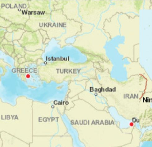

4 Mathematical Problems in Engineering

 Table 1: Comparison between the relevant literature.
 Single/multiple
Authors Fuel consumption Algorithm
 objectives
Wen et al. [16] A function of speed and payload Multiple Heuristic branch-and-price
Fagerholt et al.
 Linear interpolation Single The commercial optimization software Xpress MP
[10]
Sheng et al. [29] The third power of speed Single Formula derivation
Zhen et al. [11] Linear interpolation Single A TS-based solving method
 A hybrid strategy coupling the two-stage iterative algorithm
Zhen et al. [12] Linear interpolation Multiple
 and fuzzy logic method with ε-constraint
Cariou et al. [28] The third power of speed Single A GA-based heuristic
 Weather archive data parser and
Lee et al. [13] Multiple MOPSO
 weather impact miner
Zheng et al. [21] ANN Single PSO
Gkerekos and
 Deep neural network Single Dijkstra’s algorithm
Lazakis [14]
Ma et al. [30] The third power of speed Single Dijkstra’s algorithm
... ... ... ...
Our research LASSO regression model Multiple MOPSO

 1N 2
 minimizing formula (5), while β was solved with the LARS
 arg min p y − β0 − xTi β , (2) algorithm so that the residual error was reduced con-
 β0 ,β∈R N i�1 i
 tinuously until it was less than a constant.
 p 
 
 s.t. βj ≤ t, (3) 3.1.4. Fuel Consumption Estimation. Through the above
 j�1 analysis, a LASSO regression model was built to predict fuel
 consumption. Following the multiple linear regression
where β � (β1, β2, . . ., βp) is the regression coefficient vector formulation [36], the fuel consumption F is represented as
under sparse assumption. follows:
 Without loss of generality, the covariates can be nor-
malized so that i xij /N � 0 and i yi /N � 0. Letting y and x F � βX + b, (6)
be the mean values of yi and xi and the unbiased estimation
β 0 � y − xT β � 0. Then, by supposing the sample X � (x1, x2, where b are intercepts.
. . ., xN)T and the output vector y � (y1, y2, . . ., yN)T and
adopting the Lp norm of the vectors (‖x‖p � ( m p 1/p
 i�1 |xi | ) ), 3.2. Mathematical Model. This paper focuses on the decision
formulas (2) and (3) can be simplified as of whether to detour around the Cape of Good Hope amid
 COVID-19. The objective is to minimize to total voyage cost,
 1 �� ��2
 arg minp ��y − XβT ��2 while the voyage time is not strictly restricted. The total
 β∈R N voyage cost was broken down into the sailing fuel cost, the
 (4)
 berthing fuel cost, the charter cost, and the transit charge of
 s.t.‖β‖1 ≤ t. the Suez Canal.
 The sailing fuel cost accounts for a large proportion of
 The model can be further transformed into the Penalized the total voyage cost. Hence, it is important to predict the
Least Squares Function, which is also known as the La- sailing fuel consumption. During the voyage, the fuel
grangian form [33, 34]: consumption of the ship is affected by various eigenvari-
 1 �� ��2 ables, including but not limited to sailing speed, draft,
 L(β, λ) � minp ��y − XβT ��2 + λ‖β‖1 , (5) weather conditions, and sea conditions. Some eigenvariables
 β∈R N
 are strongly correlated, such as wind speed and wind force.
where λ is the regularization parameter (λ ≥ 0). According to The strong correlations make the fuel consumption esti-
the Lagrangian Duality, λ has a data-dependent relationship mation a typical multicollinearity problem. Hence, this
with t. paper employs the LASSO regression method proposed by
 Wang et al. [26] to select the eigenvariables and improve the
 interpretability and accuracy of the fuel consumption
3.1.3. Solving the LASSO Regression Model. The LASSO estimation.
regression model is generally solved by the combination After the LASSO regression model was determined, the
of the k-fold cross-validation and the least angle regres- mathematical model of our problem was established to
sion (LARS) algorithm (LassoLarsCV) [30, 35]. In this describe the total cost and total time of voyage and to reveal
research, λ or t is estimated by using 10-fold cross-vali- the correlation between fuel consumption, sailing speed, and
dation. λ, a constant parameter, was estimated by other factors. The two objectives of our problem are

Mathematical Problems in Engineering 5

conflicting with each other: the total voyage cost is positively subject to
correlated with the sailing speed, while the total voyage time n
is negatively correlated with the sailing speed. To rationalize l
 tarrive
 n − tleave
 1 ≥ i + tleave
 i − tarrive
 i , (9)
the decision of whether to detour, it is necessary to find the i�1
 v i
Pareto optimal solution of the tradeoff relationship between
the two objectives. The model, aiming to minimize the total Vmin ≤ vi ≤ Vmax , i � 1, . . . , n. (10)
cost and total time of voyage, was solved by the MOPSO
algorithm.
 The objective (7), minimizing the total voyage cost,
 Our research considers a liner ship operating on a given
 conflicts with the objective (8), minimizing the total voyage
route with a set of ports of call. Here, the mandatory time
 time. Constraint (9) sets a limit on the total voyage time.
window of arrival of each port is considered. However, the
 Constraint (10) ensures that the sailing speed of the ship falls
sailing speed between the two ports visited in sequence is
 between the lower and upper limits in all legs.
variable due to navigation environment and other factors.
Therefore, we set up the nodes N � {1, 2, . . ., n} including
ports that can be visited by the ship. 3.3. MOPSO Algorithm. The PSO is a metaheuristic algo-
 Each node has the arrival time tarrive
 i and the departure rithm that has been successfully applied to many real-world
time tleave
 i of the ship. For the node that is not port, we can set scenarios [37]. In the algorithm, each particle in the swarm is
tleave
 i − tarrive
 i � 0. Additionally, the trip from port i to port treated as a possible solution to the problem, and the optimal
i + 1 was defined as a leg i. The parameters of the optimi- solution is searched for based on the behaviors of particles
zation model are explained in Table 2. and the interaction between particles.
 The total voyage cost of the ship consists of three parts: Considering only one objective, the original PSO
the sailing fuel cost, berthing fuel cost, charter cost, and the proposed by Kennedy and Eberhart [38] cannot be directly
Suez Canal toll. The sailing fuel consumption for leg i was applied to multiobjective problems. The MOPSO, aimed at
described as the LASSO regression model f (vi , Ei), where Ei solving problems with different priorities, has been de-
denotes the various eigenvariables at leg i. The berthing fuel veloped in recent years, for example, handling multi-
cost per hour at port was fixed because only the auxiliary objective optimization problems with a multiswarm
engine of the ship operates during port call. Let k be the cooperative particle swarm optimizer [39], a bare-bones
mean amount of fuel consumed per hour at port. Then, the multiobjective particle swarm optimization algorithm [40],
fuel cost per hour (α) at port can be expressed as α � kPfuel. and variable-size cooperative coevolutionary particle
The charter cost depends on the total voyage time and is swarm optimization for feature selection on high-dimen-
indirectly affected by fuel price: the falling fuel price will sional data [41]. This paper selects the MOPSO framework
change the supply-demand relationship of the shipping developed by Nguyen and Kachitvichyanukul [31] as it is
market, which in turn changes the ship’s charter rate. one of the most classical MOPSO and has proven efficiency
Finally, if the ship sails through the Suez Canal, the op- for this problem. The MOPSO can memorize the current
erator must pay an expensive toll at once. Therefore, the search situation and make timely adjustment to the search
first objective of the model, seeking to minimize the total strategy, resulting in excellent global convergence and
voyage cost of the ship on the given route (M1), can be robustness.
expressed as To solve the multiobjective problem, the MOPSO
 n n mainly combines Pareto sorting mechanism to find the
 min M1 � Pfuel f vi , Ei + α tleave
 i − tarrive
 i historical optimal solution of particles and update the
 i�1 i�1
 (7) noninferior solution set. The noninferior solutions are
 n searched for in parallel using efficient clusters. In mul-
 l
 + c i + tleave
 i − tarrive
 i + Ppass y. tiobjective optimization, the MOPSO iteratively outputs a
 i�1
 v i set of noninferior solutions that are dominated by each
 other. Then, the global optimal position can be obtained
 On the given route, the voyage time of the ship should
 by randomly screening the noninferior solution set. The
be as short as possible. Therefore, the second objective is to
 steps of the MOPSO framework are summarized as
minimize the total voyage time (M2) and can be expressed
 follows:
as
 n Step 1. Z-score normalization was adopted to nor-
 l
 min M2 � i + tleave − tarrive , (8) malize the two objective functions of our problem, i.e.,
 i�1
 vi i i
 total voyage cost and total voyage time: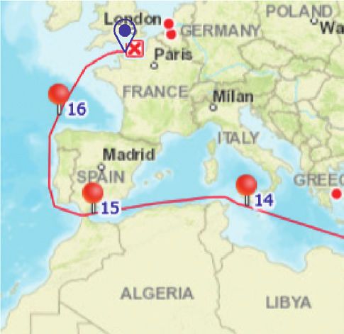

6 Mathematical Problems in Engineering

 Table 2: Notations.
Parameters Definitions
N Set of nodes N � {1, 2, . . ., n}, node i ∈ N
y A binary variable equal to 1 if the ship passes through the Suez Canal
Pfuel Fuel price per ton consumed during sailing and berthing (USD/ton)
Ppass The toll to pass through the Suez Canal (USD)
tarrive
 i Arrival time of the ship at port i (hour), tarrive
 1 � 0 is not considered
tleave
 i Departure time of the ship at port i (hour), tarrive
 n is large enough, and tleave
 n is not considered
li Sailing distance of leg i, the trip from port i to port i + 1 (nautical mile)
k Fuel consumption per hour at port (ton/hour)
c Charter rate of the ship (USD/day)
f(vi , Ei) Fuel consumption per unit time in leg i
vi Speed decision on leg i (knot)
Vmin Minimum sailing speed (knot)
Vmax Maximum sailing speed (knot)

 M1 v i − M1 v i 
 M1′ vi � ��������������������������� �, i � 1, . . . , n,
 n 2
 i�1 M1 vi − M1 vi /n − 1 
 (11)
 M2 v i − M2 v i 
 M2′ vi � ��������������������������� �, i � 1, . . . , n,
 2
 ni�1 M2 vi − M2 vi /n − 1 

 xi � xi,1 , xi,2 , . . . , xi,D ∈ RD ,
 where M1′(vi ) and M2′(vi ) are the normalized values of (13)
 M1 and M2 under speed vi , respectively, and M1 (vi ) vi � vi,1 , vi,2 , vi,D ∈ RD , i � 1, 2, . . . , n,
 and M2 (vi ) are the mean values of M1 and M2 under
 speed vi , respectively. where xi denotes the position of particle i, vi denotes the
 Step 2. The initial swarm was set up, and each particle velocity of particle i, and D is the number of decision
 was given an initial speed and position. The other variables. In the evolution process, the position and
 parameters, such as learning rate, upper and lower velocity of each particle were, respectively, updated as
 limits of inertia weight, maximum number of itera-
 tions, and swarm size, were also initialized. vk+1 k k k k k
 id � ωvid + c1 r1 pid − xid + c2 r2 pgd − xgd ,
 (14)
 Step 3. The fitness of each particle, depending on the xk+1 k k+1
 id � xid + vid ,
 two objectives, was calculated as
 ⎪
 ⎧ n n where ω is the inertia weight, k denotes the iteration
 ⎪
 ⎪ M � P f v , E + α tleave − tarrive number, r1 and r2 are uniform random variables in the
 ⎪
 ⎪ 1 fuel i i i i
 ⎪
 ⎪ i�1 i�1 interval [0, 1], d ∈ D is the dimension of the vector, pkid
 ⎪
 ⎪
 ⎪
 ⎪ and pkgd denote the acceleration constants for its per-
 ⎪
 ⎪
 ⎪
 ⎨ n
 l sonal best (P-best) and the global best position (G-
 ⎪ + c i + tleave i − tarrive
 i + Ppass y, (12) best), respectively, xkid is previous position of the
 ⎪
 ⎪ i�1
 v i
 ⎪
 ⎪ particle I, and vk+1
 ⎪
 ⎪ id is new velocity of the particle i.
 ⎪
 ⎪
 ⎪
 ⎪ n
 li Step 6. If the maximum number of iterations was
 ⎪
 ⎪ leave arrive
 ⎩ M2 � v + ti − ti .
 ⎪ reached, the set of Pareto optimal solutions was out-
 i�1 i putted; otherwise, steps 3–6 were repeated.
 Step 7. The upper and lower bounds of sailing speed
 After the algorithm was initialized and updated, the were determined according to the actual situation and
 constraints of the two objective functions were satisfied ship performance. Then, the minimum values of the
 by limiting the control variables to the specified range. two objectives (ML1 and ML2 ), i.e., the positive ideal
 Step 4. The fitness of particles was compared. The optimal point A, and the maximum values of the two objectives
 position (P-best) and noninferior solution set of particles B (MU U
 1 and M2 ), i.e., the negative ideal point B, were
 were updated according to the dominance relations. The obtained.
 global optimal position (G-best) of particles was ran- Step 8. In the set of Pareto optimal solutions, the so-
 domly selected from the noninferior solution set. lution with the minimum relative distance from pos-
 Step 5. The speed and position vectors of each of the N itive and negative ideal points was screened out as the
 particles in the swarm were, respectively, updated as optimal tradeoff solution C(M∗1 , M∗2 ), and the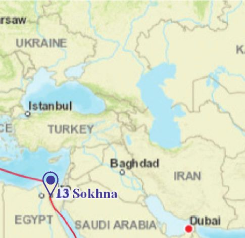

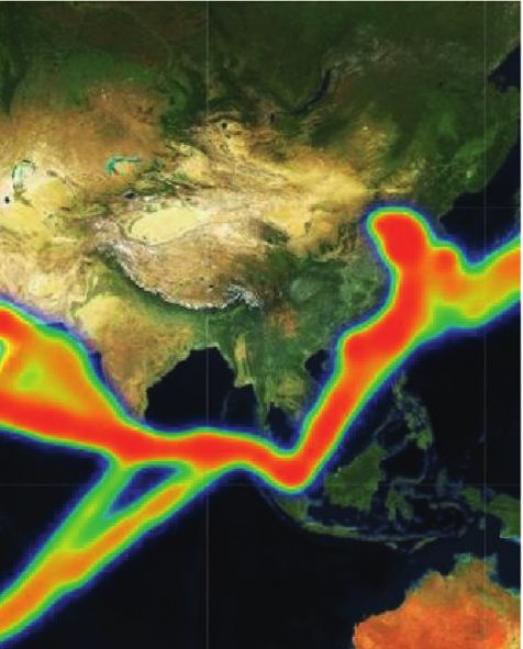
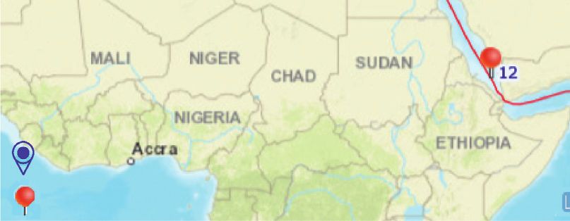
Mathematical Problems in Engineering 7

 corresponding speed was taken as the optimal sailing
 speed. Formula (15) shows the line connecting positive Negative ideal
 MU
 2 point B
 ideal point A and negative ideal point B, and the in-

 2nd objective: total sailing time
 tersection of this line and Pareto frontier is the optimal Pareto frontier
 tradeoff solution P(M∗1 , M∗2 ):

 MU L
 2 − M2
 P M∗1 , M∗2 � L L
 x − M1 + M2 , (15)
 MU − ML1 M∗2 Best trade off
 1 solution P
where P(M∗1 , M∗2 ) is the optimal tradeoff solution, ML1 and
ML2 are the minimum values of the two objectives, and MU 1 ML2
and MU 2 are the maximum values of the two objectives, Positive ideal
respectively. point A
 The selection of the best tradeoff solution from Pareto ML1 M∗1 MU
 1
frontier is shown in Figure 2. 1st objective: total cost
 Figure 2: The selection of the optimal solution from the Pareto
3.4. Weighted Sum (WS) Method. After getting the optimal frontier.
tradeoff solution of the total voyage cost and the total voyage
time though the MOPSO algorithm, the WS method [42] is
 In summary, the objective of the mathematical model in
used to evaluate two routes under specific fuel prices and
 Section 3.2 is to minimize the total fuel consumption pre-
charter rates in this paper. The purpose is to provide a
 dicted by the LASSO regression model in Section 3.1. The
decision reference for operators. The idea of the WS method
 model was solved by the MOPSO algorithm in Section 3.3.
is to convert the multiobjective optimization into a single
 Route selection was obtained through the WS method in
objective optimization problem by using a convex combi- Section 3.4. As shown in Figure 3, the algorithm is imple-
nation of objectives. The steps of the WS framework are mented in four phases: data preparation, training LASSO
summarized as follows: regression model, finding the optimal solution with the
 Step 1: the total voyage cost gap ΔM1 and the total MOPSO algorithm, and the route selection with the WS
 voyage time gap ΔM2 between the two routes in given method.
 scenario are, respectively, calculated as
 ΔM1 � M1 (1) − M1 (2), 4. Case Study
 (16)
 ΔM2 � M2 (1) − M2 (2), The data selection and preparation are introduced in Section
 4.1. The fuel consumption estimation process is presented in
 where ΔM1 is the total voyage cost gap, ΔM2 is the total Section 4.2. The setting of MOPSO parameters is shown in
 voyage time gap, ΔcM2 is the loss of economic value, U is Section 4.3. Finally, Section 4.4 gives a comprehensive
 a single objective utility function, and ω is the weight of analysis on the route choice.
 cost.
 Step 2: the total voyage time gap ΔM2 is converted into 4.1. Data Selection and Preparation. The case study uses the
 the loss of economic value ΔcM2 due to the delayed parameters of a real container ship named “CMA CGM
 delivery of the cargo in this period [16]: Chile,” which transports dry cargoes from the Indian
 τ Ocean to Le Havre, France. According to the records of the
 ΔcM2 � ΔM2 , (17)
 24 automatic identification system (AIS) provided by Elane
 Inc., the ship passed through the Suez Canal (Route SC,
 where τ is the market price of the cargo at the Figure 4) during the voyage from December 23rd, 2019, to
 destination. January 25th, 2020, departing from Qingdao, then visiting
 Step 3: the multiobjective is transformed into a single Ningbo, Daqu, Yangshan, Yantian, Pasir Panjiang, and
 objective utility function U by introducing the weight of Sokhna in sequence, and finally arriving at Le Havre.
 cost ω, which shows the route decision of operators However, the ship detoured around through the Cape of
 when they have different preferences for voyage cost Good Hope (Route CGH, Figure 5) during another voyage
 and voyage time. The WS method solves the scalar from March 16th, 2020, to April 25th, 2020. The order of
 optimization problem: ports visited by the ship was Qingdao, Ningbo, Daqu,
 Yangshan, Yantian, Pasir Panjiang, and Le Havre. Al-
 though the ship detoured around through the Cape of
 min U � ωΔM1 +(1 − ω)ΔcM2 , (18) Good Hope, the ports visited in actual voyage did not
 change. Therefore, it is appropriate for this paper to select
where 1 ≥ ω ≥ 0. such a range of ship navigation for calculation. In addition,

8 Mathematical Problems in Engineering

 Reading operation data from

 Data preparation
 automatic identification
 Sailing data system (AIS) Weather/sea data

 Course/speed/ Waves/currents/
 draft/… wind/salinity/…

 Training LASSO model
 Data segmentation Training data
 LassolarsCV
 Normalized data
 algorithm
 Test data

 Fuel consumption Sparse LASSO
 prediction model regression model

 Alternative routes Fuel price, charter rate, toll, …

 New input value Evaluating objective values:
 Initializing particles with random

 MOPSO algorithm
 minimum voyage cost;
 positions and zero speed
 minimum voyage time

 Updating speed and Determining global non
 position dominated front
 Fitness value
 Selecting guidance No Yes
 Meeting termination criterion? End
 from elite group

 Route (1) SC Route (1) CGH
 The total voyage cost M1 (1) The total voyage cost M1 (2)
 The total voyage time M2 (1) The total voyage time M2 (2)

 Weighted sum (WS) method
 Yes
 Route (1) SC ΔM1 = M1(1) – M1(2) < 0? ΔM2 = M2(1) – M2(2) < 0

 No Convert time to cost

 The total voyage cost gap ΔM1 The lost income Δ‘M2

 Yes
 Route (1) SC U < 0? Utility function U
 N
 Route (2) CGH

 Figure 3: The workflow of the method in the paper.

several legs except the legs between the ports of call in 2020). In addition, the arrival time tarrive
 i and the departure
actual voyage are given in the figures to prove the fuel time tleave
 i of the ship at node i were obtained from AIS data.
consumption estimation model proposed. Here, the market price of the cargo at the destination
 Here, the fuel costs of the two routes were estimated τ � 10000 USD/day. Finally, the maximum and minimum
based on two different fuel prices: Pfuel � 365.5 USD/ton (the sailing speeds were taken from the shipping logs. The values
fuel price in March 20, 2019) and Pfuel � 190.6 USD/ton (the of the related parameters are listed in Table 3.
fuel price in December 27, 2019). The berthing fuel con-
sumption per hour is set as k � 5.2 ton/hour [28]. The detour
will increase the total voyage time, incurring more charter 4.2. Fuel Consumption Estimation. The main dataset avail-
cost, and the charter rate is affected indirectly by the fuel able from AIS and ocean dataset includes mean speed, mean
price. Here, the charter cost is set to 20,833.3 USD/day at the draft, course, current speed, wind speed, wind force, sea-
fuel price of 190.6 USD/ton [43]. The toll to pass through the water temperature, seawater salinity, and effective wave
Suez Canal is set to 450,000 USD (the toll in January 4th, height. Among them, the weather data like current speed,

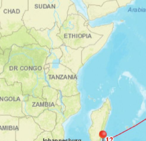
Mathematical Problems in Engineering 9

 N

 Ports of call in actual voyage
 Nodes that can be visited by the ship

Figure 4: Route SC before the falling of fuel price (sailing from December 23rd, 2019, to January 25th, 2020, passing through the Suez
Canal).

 N

 Ports of call in actual voyage
 Nodes that can be visited by the ship
Figure 5: Route CGH after the outbreak of COVID-19 (sailing from March 16th, 2020, to April 25th, 2020, around the Cape of Good Hope).

 Table 3: The values of relevant parameters. normalization. The normalized dataset was randomly di-
Parameters Value vided into a training set and a test set at the ratio of 4 : 1 and
Fuel consumption per hour at used to verify the effectiveness and reliability of our esti-
 5.2 tons/hour mation model.
port, k
 20,833.3 USD/day at the fuel Taking fuel consumption as the response and other
Charter rate, c
 price of 190.6 USD/ton eigenvariables as inputs, our estimation model was opti-
Maximum sailing speed, Vmax 22 knots mized by computing the best λ conforming to the least RSS.
Minimum sailing speed, Vmin 10 knots As mentioned in Section 3.1.3, 10 equal subsets were divided
The toll to pass through the from the training set and conducted for validation. In this
 450,000 USD
Suez Canal, Ppass way, the optimal values of λ and b were determined as
 0.020955 and 0.0000928, respectively.
wind speed, wind force, and seawater temperature were In this case study, the five eigenvariables (as marked by ∗
extracted from the nc.file obtained from the Copernicus in Table 6) corresponding to the nonzero regression coef-
Marine Environment Monitoring Service [44]. Part of the ficients were selected for fuel consumption estimation. As
original dataset is presented in Table 4. shown in Table 6, the eigenvariables were loosely correlated
 The original dataset, involving 490 samples and 10 with fuel consumption, except for sailing speed. The
eigenvariables, was used to train our model. Table 5 shows eigenvariables like current speed, wind speed, and wind
the original dataset after being processed by Z-score force had very small effects on fuel consumption. The sailing

10 Mathematical Problems in Engineering

 Table 4: Part of the original dataset of the ship.
Number Fuel consumption (ton) Sailing speed (knot) Draft (m) Wind speed (m/s) Wind force (Pa) Seawater salinity (0.001) . . .
1 4.14 11.88 11.7 3.47 0.02 28.12
2 4.74 12.42 11.7 4.09 0.03 29.22
3 5.01 12.64 11.7 4.22 0.03 31.51
 ...
4 6.51 13.1 11.7 5.23 0.04 32.63
5 6.33 13.5 11.7 5.15 0.04 32.42
... ... ... ... ... ... ...

 Table 5: Part of the normalized dataset of the ship.
Number Fuel consumption Sailing speed Draft Wind speed Wind force Seawater salinity ...
1 −2.2605 −2.5564 −4.8435 −1.0858 −0.8543 −3.6283
2 −2.1378 −2.3163 −4.8435 −0.8737 −0.7193 −3.0492
3 −2.0846 −2.2185 −4.8435 −0.8292 −0.7193 −1.8437
 ...
4 −1.7787 −2.0140 −4.8435 −0.4835 −0.5844 −1.2541
5 −1.8170 −1.8361 −4.8435 −0.5109 −0.5844 −1.3647
... ... ... ... ... ... ...

Table 6: Regression coefficient vector of our estimation model. that can be applied to all ships, indeed, which is even im-
Features βi
 possible. Now, it can be shown that the LASSO algorithm is
 able to estimate the fuel consumption of the test ship with
Sailing speed 0.9591∗
 considerable precision. The rest of the case study is to apply
Draft 0.0022∗
Course 0 the MOPSO algorithm based on the estimated fuel con-
Wind speed 0 sumption model.
Wind force −0.0018∗
Current direction (east) 0
Current direction (north) −0.2678∗
 4.3. Setting of MOPSO Parameters. The MOPSO parameters
Wave height 0 were configured as follows: the swarm size N is 200, and the
Seawater salinity −0.0366∗ maximum number of iterations is 100. Under this setting,
Seawater temperature 0 the program took 47 seconds on average in 30 repeated runs.
 In 24 out of the 30 runs, the results were basically consistent,
 indicating the stability of the MOPSO algorithm. Figure 8
speed makes the greatest impact on the fuel consumption. As shows the convergence curves of the two objective functions.
a result, the fuel consumption cost increases significantly It can be seen that the MOPSO algorithm had converged to
with sailing speed, which can also increase the total voyage the optimal values of the two objectives at the 100th iteration.
cost. The correlations of the selected eigenvariables are also
illustrated in Figure 6. The LASSO regression model solves 4.4. Results and Discussion
the multicollinearity between variables, as evidenced by the
strong correlation between wind speed and wind force. 4.4.1. Analysis on the Current Situation: Why Detour?
 A comparison between our estimation model and a Recall the phenomenon introduced in Section 4.1 that the
general linear regression estimation is provided to verify the ship “CMA CGM Chile” sailed through Route SC at a fuel
performance. The estimation effects of the two models on the price of 365.5 USD/ton and detoured to Route CGH at a fuel
same test set were measured by the mean absolute per- price of 190.6 USD/ton. By using our proposed algorithms,
centage error (MAPE) and root mean square error (RMSE) we are able to explain why the ship chose to detour. As
(Table 7). The fitting performance of the two methods is shown in Figure 9, the optimal solutions of both Route SC
compared in Figure 7. Apparently, our model outperformed (depicted in green) and Route CGH (depicted in red) follow
the general linear regression model in the estimation of fuel the pattern that the total voyage cost decreases with the total
cost and achieved lower RMSE and MAPE than that model. voyage time rising. Since the decision-maker has to choose
 Compared with Wang et al. [26], another study utilizes from the optimal solutions, it is clear that the two objectives,
LASSO-based model for ship fuel consumption and achieves minimizing the total voyage cost and minimizing the total
a RMSE of 7.4, and the performance of our model seems voyage time, conflict with each other. In order to make
better. While the workflows of LASSO algorithm in two comparison among the optimal solutions in Route SC and
papers are similar, the RMSE value depends on the data Route CGH, we applied the principle of selecting the optimal
selection. Wang et al. [26] collected data from 97 ships with solution from the Pareto frontier in Section 3.3.
different sizes. In contrast, our paper focuses on only one Figure 9(a) displays the total voyage cost and total voyage
ship (CMA CGM Chile), in order to achieve the best ac- time of Route SC at the fuel price of 365.5 USD/ton. It can be
curacy on this ship and precisely simulate the routing de- seen that the total voyage cost of the Pareto optimal solution
cision. Our aim is not to develop a general fuel consumption was 2,711,000 USD, and the total voyage time was 793.3

Mathematical Problems in Engineering 11

 1.00
 Speed 1 0.47 0.041 0.055 0.13 –0.13 –0.0014 0.42 0.25

 draft 0.47 1 0.064 0.077 0.32 –0.098 –0.072 0.41 0.27
 0.75

 Wind speed 0.041 0.064 1 0.94 0.52 –0.098 –0.24 –0.13 0.12

 Wind force 0.055 0.077 0.94 1 0.52 –0.044 –0.23 –0.1 0.13
 0.50

 Wave height 0.13 0.32 0.52 0.52 1 –0.18 –0.19 0.052 0.18

 Current direction
 –0.13 –0.098 –0.098 –0.044 –0.18 1 0.14 –0.13 –0.031 0.25
 (east)

 Current direction
 –0.0014 –0.072 –0.24 –0.23 –0.19 0.14 1 –0.015 1.4e–05
 (north)

 Temperature 0.42 0.41 –0.13 –0.1 0.052 –0.13 –0.015 1 –0.085 0.00

 Salinity 0.25 0.27 0.12 0.13 0.18 –0.031 1.4e–05 –0.085 1

 (east)
 Speed

 Draft

 Wind speed

 Wind force

 Wave height

 Current direction

 Current direction
 (north)

 Temperature

 Salinity
 Figure 6: The correlations between eigenvariables.

 Table 7: Comparison of MAPE and RSME values of the two models.
Model MAPE (%) RMSE
Our model 9.2482 1.6458
General linear regression model 19.9612 3.1275

 35 35

 30 30

 25 25

 20 20

 15 15

 10 10

 5 5

 0 0
 0 100 200 300 400 0 100 200 300 400
 Sample no. Sample no.

 Actual fuel consumption of the voyage Actual fuel consumption of the voyage
 Predicted fuel consumption of the voyage Predicted fuel consumption of the voyage
 (a) (b)

 Figure 7: Comparison of estimation results of the two models: (a) our model; (b) general linear regression model.

12 Mathematical Problems in Engineering

 ×106
 2.85 820

 2.8 810

 2.75
 800

 2nd objective
 1st objective

 2.7
 790
 2.65
 780
 2.6

 770
 2.55

 24/30 24/30
 2.5 760
 0 20 40 60 80 100 0 20 40 60 80 100
 Iterations Iterations
 (a) (b)

 Figure 8: Convergence curves of the two objective functions: (a) first objective; (b) second objective.

 935
 940
 X 2849000 935
 925 X 1696000
 Y 919.9
 930 Y 928.8
 915
 925
 Voyage time (hours)

 Voyage time (hours)

 905 920
 126.6 915 140.2
 820
 805
 810

 800 X 2711000 795 X 1822000
 Y 793.3 –126,000 Y 788.6
 790 785
 138,000
 780
 775
 770
 2.62 2.65 2.7 2.75 2.8 2.84 2.88 2.92 1.67 1.68 1.69 1.70 1.71 1.72 1.79 1.81 1.83 1.85
 Total voyage cost (USD) ×106 Total voyage cost (USD) ×106

 Optimal solution set of route SC Optimal solution set of route SC
 Optimal solution set of route CGH Optimal solution set of route CGH

 (a) (b)

Figure 9: The distribution charts of total voyage cost and total voyage time of the two routes at the fuel price of (a) 365.5 USD/ton and
(b) 190.6 USD/ton.

hours. As shown in Figure 9(a), the total voyage cost of USD/ton and 126,000 USD lower than that of Route SC.
Route CGH stood at 2,849,000 USD, and the total voyage Although the total voyage time of Route CGH at the fuel
time lasted 919.9 hours. Route CGH had a greater total price of 190.6 USD/ton was 140.2 hours (about 5.8 days)
voyage cost and total voyage time than Route SC. Hence, it is longer than that of Route SC, by balancing the different
more cost-effective to choose Route SC at the fuel price of objectives, the ship chose the longer route at the fuel price
365.5 USD/ton. of 190.6 USD/ton.
 After the outbreak of COVID-19, the global fuel price Table 8 compares the voyage time and speed of each
plunged deeply. Figure 9(b) displays the total voyage cost leg on two routes that were estimated by using the
and total voyage time of Route SC at the fuel price of 190.6 methodology proposed in this paper, and the actual
USD/ton. The total voyage cost was 1,822,000 USD, much values collected from AIS data. The relative error of
smaller than that in the scenario of 365.5 USD/ton. And the voyage time and speed was limited to less than 9%, except
total voyage cost of Route CGH was 1,696,000 USD, down for Leg 7 of Route CGH in the scenario of 190.6 USD/t. It
by 1,153,000 USD/ton from that at the fuel price of 365.5 also can be seen that the sailing speed fluctuated during

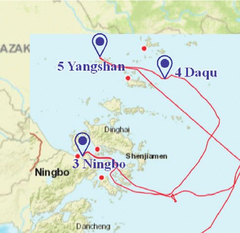
Mathematical Problems in Engineering 13

 Table 8: Estimation and actual values of the variables of each leg on two routes.
 Actual voyage Estimated voyage Relative error of Actual Estimated Relative error of
 Leg i
 time (hour) time (hour) voyage time (%) speed (knot) speed (knot) speed (%)
 Leg 1 22.13 21.39 −3.37 12.19 12.62 3.49
 Leg 2 24.70 24.45 −1.03 10.98 11.09 1.04
 Leg 3 9.33 10.10 8.18 12.32 11.39 −7.56
 Leg 4 3.88 3.64 −6.24 7.21 7.69 6.65
 Leg 5 21.63 22.60 4.48 17.23 16.49 −4.28
 Leg 6 23.37 25.34 8.47 18.24 16.82 −7.80
 Leg 7 35.03 37.66 7.49 19.10 17.77 −6.97
Fuel price of 365.5 Leg 8 46.97 47.39 0.90 17.09 16.94 −0.89
USD/t, Route SC Leg 9 77.65 75.81 −2.37 18.73 19.18 2.42
 Leg 10 69.92 71.95 2.90 17.97 17.46 −2.82
 Leg 11 68.58 68.26 −0.46 17.90 17.98 0.47
 Leg 12 60.95 59.41 −2.52 16.76 17.19 2.59
 Leg 13 66.80 67.94 1.70 16.67 16.39 −1.67
 Leg 14 46.75 46.67 −0.16 19.03 19.06 0.16
 Leg 15 40.33 37.90 −6.04 17.74 18.88 6.43
 Leg 16 48.65 44.72 −8.08 10.64 11.57 8.79
 Leg 1 13.32 14.17 6.40 13.37 12.57 −6.01
 Leg 2 31.12 31.46 1.11 11.14 11.02 −1.09
 Leg 3 9.17 8.62 −5.93 12.44 13.22 6.30
 Leg 4 3.83 3.67 −4.20 7.72 8.06 4.38
 Leg 5 28.68 29.87 4.12 17.11 16.43 −3.96
 Leg 6 26.47 24.31 −8.14 11.97 13.03 8.86
 Leg 7 38.05 44.11 15.93∗ 18.66 16.10 −13.74∗
Fuel price of 190.6 Leg 8 42.92 41.81 −2.57 17.84 18.31 2.64
USD/t, Route CGH Leg 9 66.82 65.91 −1.35 18.15 18.40 1.37
 Leg 10 63.57 64.05 0.77 18.07 17.93 −0.76
 Leg 11 89.60 88.15 −1.62 17.80 18.09 1.65
 Leg 12 89.23 86.99 −2.51 17.29 17.73 2.57
 Leg 13 87.42 90.91 3.99 18.83 18.11 −3.84
 Leg 14 96.78 95.09 −1.75 19.35 19.70 1.78
 Leg 15 79.60 74.90 −5.90 18.70 19.87 6.27
 Leg 16 64.22 65.66 2.25 17.61 17.22 −2.20

Leg 1∼16 of the voyage. When sailing for a short distance represented by yellow rectangles in Figure 11. The actual
on Leg 1∼4, the speed obtained by the model is basically combinations of fuel price and charter rate were repre-
consistent with the actual speed. Similarly, when sailing sented by blue dots. Then, the total voyage cost and the
for a long distance on Leg 5∼16, the estimated values is relationship between the four scenarios were analyzed in
also close to the actual values. In a word, the estimations details.
and the actual values are basically the same. The results Table 9 provides the total voyage costs and the total
again prove that our methodology can precisely predict voyage time of Route SC and Route CGH in Scenarios
the actual voyage. HFHC, HFLC, LFHC, and LFLC, respectively. In Sce-
 narios HFHC, LFHC, and HFLC, the total voyage cost of
 Route SC was at least 120,700 USD, 83,700 USD, and
4.4.2. Scenario Analysis: When to Detour? The fuel prices 130,300 USD lower than that of Route CGH, as shown in
and charter rates are time-varying factors. Figure 10 the inputs that were marked by ∗ in Table 9, and Route SC
shows the change in fuel price and charter rate from remains an absolute advantage on the total voyage time
December 20th, 2019, to July 3rd, 2020, collected from due to the sailing distance. Therefore, the operator will
Clarksons [43]. According to the actual distributions of naturally choose Route SC in the above three scenarios. By
fuel price and charter rate, four scenarios were designed contrast, in Scenario LFLC, the total voyage cost of Route
(Figure 11): high fuel price and high charter rate (HFHC), SC was higher than that of Route CGH for all fuel price
high fuel price and low charter rate (HFLC), low fuel and charter rate although the total voyage time of Route
price and high charter rate (LFHC), and low fuel price SC took less time, as shown in the inputs corresponding to
and low charter rate (LFLC). Although the HFLC sce- LFLC in Table 9, marked by ∗. In this case, it should
nario happens occasionally in reality, this scenario was analyze the operator’s preference to find out which route
simulated to provide more comprehensive results. The will be more competitive. And if let the operator select
combinations of fuel price and charter rate in HFLC were Route SC in Scenario LFLC, how does the authority of the
generated randomly within the range of HFLC and Suez Canal need to adjust its canal toll?

14 Mathematical Problems in Engineering

 HFHC LFHC LFLC HFLC
 400 35000

 350 30000

 Charter rate (USD/day)
 Fuel price (USD)
 300 25000

 250 20000

 200 15000

 150 10000

 2019/12/20 2020/07/03
 Date

 Charter rate Fuel price
 Simulated charter rate Simulated fuel price
 Figure 10: The change trend of fuel price and charter rate.

 35000
 LFHC HFHC
 Charter rate (USD/day)

 30000

 25000

 20000

 15000
 LFLC HFLC
 10000
 150.0 200.0 250.0 300.0 350.0 400.0
 Fuel price (USD/ton)

 Combinations of actual fuel price and charter rate
 Simulated combinations of fuel price
 and charter rate in HFLC
 Figure 11: The four scenarios.

 Actually, the canal toll is a significant factor influ- by the WS method, as mentioned in Section 3.4. The
encing the route choice when fuel price and charter rate higher the value of U, the more attractive the Route SC.
are fixed. On April 1st, 2020, the authority of the Suez The results of ΔM1 , ΔM2 , and U are shown in Table 10. We
Canal once announced a 6% discount for European ships also calculated the Suez Canal toll (Ppass) and the toll
[45], but it is evident with many ships including the CMA discount corresponding to U = 0, which can make sure the
ship that this discount is not sufficient to prevent the attractiveness of Route SC and Route CGH are the same,
detour around the Cape of Good Hope. Here, taking the by linearly interpolating a value between the Suez Canal
fuel price of 193.58 USD/ton and the charter rate of 20,500 tolls with utilities very close to zero. In Table 10, the
USD/day in April 3rd, 2020, as an example in the Scenario positive U that was closest to zero and the negative U that
LFLC set, we attempted to test the impact of different was closest to zero under any cost preference were marked
discounts on the original canal toll (450,000 USD) on the by ∗, and the Ppass corresponding to U=0 was derived
choice between Route SC and Route CGH using the WS from these values.In order to avoid the ships from
method in Section 3.4. The route choice decision-making detouring to Route CGH, the Suez Canal Authority needs
is complicated by the fact that the adjustment of canal toll to keep U ≥ 0 when adjusting Ppass and the toll discount.
impacts both the total voyage cost gap ΔM1 and the total From the results in Table 10, we can find two im-
voyage time gap ΔM2 between the two routes. Therefore, plications. First, if the operator does not pay so much
we used utility (U) to represent the satisfactory degree of attention to the voyage cost, even if the canal toll does not
the decision-maker. The values of utility can be calculated need to be discounted, that is, when it is still 450000 USD,

Mathematical Problems in Engineering 15

 Table 9: The total voyage cost and total voyage time of two routes in the four scenarios.
 The total voyage
 Fuel The total The total The total The total The total voyage
 Charter cost gap between
 price voyage cost of voyage cost of voyage time voyage time time gap between
Scenarios rate (USD/ Route SC and
 (USD/ Route SC (104 Route CGH of Route SC of Route Route SC and
 day) Route CGH (104
 ton) USD) (104 USD) (hour) CGH (hour) Route CGH (hour)
 USD)
 340.50 28,500 266.17 279.03 −12.87 792.1 925.3 −133.2
 365.50 28,500 271.11 284.90 −13.80 793.3 919.9 −126.6
 361.42 28,500 268.17 280.87 −12.70 791 920.5 −129.5
 379.75 29,500 283.23 302.20 −18.97 786.9 921.0 −134.1
 372.25 30,000 293.60 312.93 −19.33 788.2 922.3 −134.1
 374.00 30,000 297.17 316.63 −19.47 790.2 922.4 −132.2
HFHC
 353.50 30,000 276.83 294.60 −17.77 784.5 921.0 −136.5
 344.17 30,500 274.00 289.63 −15.63 781.0 923.0 −142
 326.50 29,500 263.20 278.17 −14.97 782.1 925.6 −143.5
 334.00 29,000 266.10 279.87 −13.77 788.5 930.1 −141.6
 305.08 29,000 256.77 268.83 −12.07∗ 778.3 926.1 −147.8
 309.00 27,000 250.07 262.60 −12.53 774.6 936 −161.4
 218.17 26,000 214.87 223.23 −8.37∗ 757.1 931.2 −174.1
LFHC 191.42 24,500 200.20 209.93 −9.73 773.2 917.5 −144.3
 197.75 23,000 197.00 205.53 −8.53 763.3 916.9 −153.6
 193.58 20,500 189.53 175.97 13.56∗ 775.8 928.5 −152.7
 206.33 20,000 191.83 174.03 17.80∗ 780.4 921.0 −140.6
 191.17 19,500 185.97 167.13 18.84∗ 788.6 928.8 −140.2
 163.42 17,500 169.27 156.17 13.10∗ 782.5 912.5 −130
 163.25 17,000 164.50 154.27 10.23∗ 780.6 920.0 −139.4
 181.17 16,500 170.50 149.77 20.73∗ 779.4 908.5 −129.1
 173.08 15,000 160.47 147.83 12.64∗ 777 905.0 −128
LFLC
 213.00 14,500 162.57 154.63 7.94∗ 771 893.1 −122.1
 208.75 14,000 172.93 150.30 22.63∗ 781.2 900.3 −119.1
 242.50 12,500 180.17 162.10 18.07∗ 780.9 921.5 −140.6
 256.50 11,500 185.37 162.57 22.80∗ 791.5 924 −132.5
 251.00 16,000 193.47 168.17 25.30∗ 786.5 915.8 −129.3
 257.50 16,750 199.50 175.53 23.97∗ 779.8 916.4 −136.6
 261.83 17,500 208.50 185.93 22.57∗ 786.6 915.2 −128.6
 305.00 21,000 235.10 248.13 −13.03 790.2 926.5 −136.3
HFLC 319.50 21,500 245.70 259.37 −13.67 791.5 928.0 −136.5
 345.40 20,500 232.67 248.40 −15.73 796.1 931.8 −135.7

Route SC still has obvious competitiveness. For example, of the operator’s preference. Only when the operator pays
we can clearly observe that when the operator’s cost more attention to the cost preference, the authority of the
preference is reduced to 0.3, that is, when the operator Suez Canal needs to have more discount for the canal toll
pays more attention to the loss of economic value caused if the operator wants to choose Route SC. For example,
by the delayed delivery of the cargo, the operator will when the cost preference equals 1, the authority of the
undoubtedly choose Route SC. That is to say, if the arrival Suez Canal needs to give a discount of more than 30.13%
time of the ship at the destination becomes very im- (as marked by ∗ in the bottom of Table 10) on the canal
portant, that is, when the operator is not allowed to toll to make a difference in the route choice of the op-
violate the delivery agreement, the ship will not detour erator. As previously analyzed, the cost preference of 0.3
Route CGH. However, April 2020 is in a relatively special can no longer be discounted. So, for the cost preference
time window. COVID-2019 triggered many chain reac- of 0.4, the authority of the Suez Canal only needs to
tions in the global shipping market. Factor in some reduce the canal toll to 40830USD; that is, 9.27% dis-
operators had no time to pay attention to delivery of the count (as marked by ∗ in the bottom of Table 10) is
cargo in transit, many ports were closed down, and the enough to enable the ship to re-enter Route SC.
fluctuation of fuel price and charter rate was abnormal. Finally, we do a computational experiment on the canal
Route CGH became a cost-saving choice for some op- toll discounts which should be made by the authority of the
erators at that time. Suez Canal for the operator with different preferences under
 The second implication is that if the authority of the all possible fuel prices and charter rates in the Scenario LFLC
Suez Canal is willing to discount the canal toll, it will set. The results in Table 11 show that when the operator's
certainly have an effect on the route selection, regardless cost preference is higher than 0.5, the canal toll discount