Application of Machine Learning for Fenceline Monitoring of Odor Classes and Concentrations at a Wastewater Treatment Plant
←
→
Page content transcription
If your browser does not render page correctly, please read the page content below
sensors
Article
Application of Machine Learning for Fenceline Monitoring of
Odor Classes and Concentrations at a Wastewater
Treatment Plant
Federico Cangialosi *, Edoardo Bruno and Gabriella De Santis

                                          Tecnologia e Ambiente (T&A), 8-70017 Putignano, Italy; e.bruno@tecnologiaeambientesrl.com (E.B.);
                                          g.desantis@tecnologiaeambientesrl.com (G.D.S.)
                                          * Correspondence: federico.cangialosi@icloud.com; Tel.: +39-080-4055162

                                          Abstract: The development of low-cost sensors, the introduction of technical performance specifica-
                                          tions, and increasingly effective machine learning algorithms for managing big data have led to a
                                          growing interest in the use of instrumental odor monitoring systems (IOMS) for odor measurements
                                          from industrial plants. The classification and quantification of odor concentration are the main goals
                                          of IOMS installed inside industrial plants in order to identify the most important odor sources and
                                          to assess whether the regulatory thresholds have been exceeded. This paper illustrates the use of
                                          two machine learning algorithms applied to the concurrent classification and quantification of odors.
                                          Random Forest was employed, which is a machine learning algorithm that thus far has not been used
                                          in the field of odor quantification and classification for complex industrial situations. Furthermore,
                                          the results were compared with commonly used algorithms in this field, such as artificial neural
                                          network (ANN), which was here employed in the form of a deep neural network. Both techniques

                                   were applied to the data collected from an IOMS installed for fenceline monitoring at a wastewater
                                          treatment plant. Cohen’s kappa and Normalized RMSE are used as specifical performance indicators
Citation: Cangialosi, F.; Bruno, E.;
De Santis, G. Application of Machine
                                          for classification and regression: the indicators were calculated for the test dataset, and the results
Learning for Fenceline Monitoring of      were compared with data in the literature obtained in contexts of similar complexity. A Cohen’s
Odor Classes and Concentrations at a      kappa of 97% was reached for the classification task, while the best Normalized RMSE, namely 4%,
Wastewater Treatment Plant. Sensors       for the interval 20–2435 ouE/m3 was obtained with Random Forest.
2021, 21, 4716. https://doi.org/
10.3390/s21144716                         Keywords: electronic nose; instrumental odor monitoring system; odor classification; odor quantifi-
                                          cation; multilayer perceptron; random forest
Academic Editor: Victor Sysoev

Received: 11 June 2021
Accepted: 8 July 2021
                                          1. Introduction
Published: 9 July 2021
                                               Odors are a relevant component of atmospheric pollution and an important indicator
                                          of the health of urban areas close to urban wastewater treatment plants (WWTPs) [1]. As a
Publisher’s Note: MDPI stays neutral
with regard to jurisdictional claims in
                                          result of the continuous expansion of cities, these plants are located closer to residential
published maps and institutional affil-
                                          receptors, sometimes at distance of less than 500 m to 1 km. Moreover, urban WWTPs
iations.
                                          in the EU are not subject to the Industrial Emission Directive (IED) 2010/75/EU or the
                                          related Best Available Techniques to avoid the emission of odors, nor have maximum
                                          allowable odor concentrations been established. Although no legislation regulating odor,
                                          with specific requirements on odor emissions from sources, is in force in Europe, America,
                                          or Australia, various regions within certain member states in the EU have implemented
Copyright: © 2021 by the authors.
                                          their own regulations in order to define discharge limits from sources and how odor
Licensee MDPI, Basel, Switzerland.
                                          pollution issues for urban WWTPs should be managed [2–4].
This article is an open access article
distributed under the terms and
                                               In such a complex and socially sensitive context due to the various reports of bad
conditions of the Creative Commons
                                          odors in the proximity of urban WWTPs, the contribution of citizen science for identifying
Attribution (CC BY) license (https://     odor emissions [5–7] and the electronic nose or Instrumental Odor Monitoring System
creativecommons.org/licenses/by/          (IOMS) [8] are powerful tools to help policy makers and environmental protection agencies
4.0/).

Sensors 2021, 21, 4716. https://doi.org/10.3390/s21144716                                                   https://www.mdpi.com/journal/sensors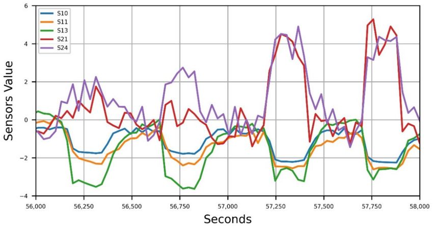
Sensors 2021, 21, 4716                                                                                          2 of 17

                         define appropriate strategies or specific prescriptions on a case-by-case basis in order to
                         identify, measure, and reduce the impact of odors on receptors.
                               IOMS offer advantages over dynamic olfactometers because they are designed for
                         real-time measurements [9,10] and do not suffer from the limitations of citizen science
                         approaches, such as biased information and high variability of results [11]. Furthermore,
                         the rapid development of low-cost sensors, which allows for air pollution monitoring
                         at a lower cost and with a higher spatial density than reference measurement methods,
                         the work undertaken by the Technical Committee CEN/TC 264 “Air quality” and the
                         relative working group (WG41) for defining technical specifications for the performance
                         evaluation of air quality sensors, and the development of the high-speed communications
                         network (5G) are the most significant recent developments for the field of IOMS hardware.
                         The software developments in recent years are remarkable both in the field of data pre-
                         treatment and feature extraction [12,13], and algorithms for odor classification [14,15] and
                         quantification [16]. Several machine learning (ML) algorithms were proposed for pattern
                         recognitions of odor, such as PCA, LDA, ANN, PLS, and SVM, and these were employed
                         as regression techniques in order to obtain odor concentrations [17–19]. However, most
                         software developments, including the recent use of Random Forest classification [20], were
                         achieved in the laboratory or in controlled situations, where the environmental conditions
                         (relative humidity and temperature) relevant in the environmental monitoring of odor
                         emissions were not considered.
                               On the other hand, performance validation of IOMS for odor classification and con-
                         centration analyses for complex situations with several odor sources have been carried
                         out in the last few years with promising results. This enables valuable information to
                         be gathered on the time variations of odors from the sources [21–23]. However, in such
                         case studies, little detail is provided on the algorithms employed for odor classification
                         and regression, and the performance indicators for classification and regression are not
                         extensively discussed. In other words, in the literature, there are several studies in which
                         ML algorithms for odor classification and quantification are discussed and compared in
                         controlled situations or for the purposes of production quality control [24–26]; however,
                         in the field of environmental monitoring applications, such information is lacking, and
                         only the direct comparison of the results of commercial IOMS with real data is shown [27],
                         without any information on the algorithms employed to derive the measurements. In the
                         near future, information on the algorithms employed, feature selection, training procedures,
                         cross-validation, and test set-related performance indicators could be essential when a
                         commercial or prototype IOMS is installed in the field, which are far more relevant for
                         the final measurement than the sensor characteristics. Moreover, field IOMS applications
                         for environmental monitoring are discussed in the literature for environmental monitor-
                         ing of either odor concentrations only or odor classification only, with few simultaneous
                         monitoring applications [22]. Moreover, the ones that exist lack detailed information on
                         the algorithms used. Only recently has an application of IOMS in complex industrial
                         plants with qualitatively and quantitatively different emission sources been thoroughly
                         discussed with reference to the ML algorithms employed for concurrent odor classification
                         and quantification [28].
                               The main goal of this work was to describe a field IOMS application for the simul-
                         taneous monitoring of odor concentrations and classes in an urban WWTP, in which the
                         ML algorithms employed are described in detail, with reference to Random Forest, which
                         thus far has not been used in the field of odor quantification and classification for complex
                         industrial situations. In detail, as part of a project for monitoring odor emissions from
                         urban WWTPs and the related sources [29], a dataset of odor classes and concentrations
                         was created, consisting of samples collected by different sources of odor emissions from
                         WWTPs, each with time-varying concentrations. This research discusses training and
                         testing of an IOMS coupled with two Machine Learning algorithms developed for the
                         purpose: an artificial neural network (Multilayer Perceptron, MLP) and Random Forest
                         (RF), the former having already been employed for IOMS operating for fenceline odor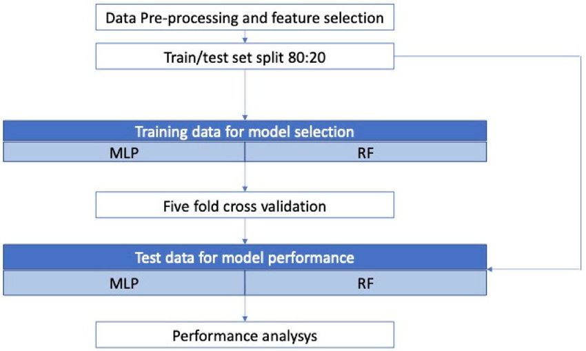
Sensors 2021, 21, 4716 3 of 17
monitoring [30,31], while the latter has yet to be used for odor classification or regression
in environmental applications. Both techniques were applied to the data collected from an
IOMS installed for fenceline monitoring at a WWTP. The results obtained from the models
are discussed, and performance parameters for classification and regression were identified
and quantified.
2. Materials and Methods
2.1. Odor Emission Source Characterization
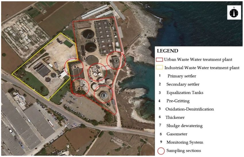
The urban WWTP here considered is located in the industrial area of Monopoli (Bari–
Italy), which is designed for a 64,695 population equivalent (PE) and operating with an
average daily flow of 12,939 m3 /d (Figure 1). The plant is located at a distance of 420 m
from the closest residential buildings.
Figure 1. WWTP of Monopoli, indicating the sampling points.
On the basis of the data from various studies carried out for the odor characterization
of WWTPs [9,32], it was established that the most critical sections are pretreatments,
primary sedimentation, and sludge conditioning. On the basis of such studies and evidence
gathered in the field, WWTP odor mapping was carried out: the first phase comprised a
complete characterization of the emission sources, and subsequently, a sampling program
of the most critical sources was defined. The sampling program for collecting samples for
training and testing was designed in order to take into account environmental variations
in the ambient air (temperature, relative humidity). Thus, it lasted several months: from
October to April.
As a result of regional enforcement [4,33], the sections of pretreatment and sludge
thickening were covered, depressurized, and the air was treated in two biofilters; moreover,
an anaerobic digester for sludge was active, which was associated with energy recovery by
combustion, so that even biogas may be an important source of fugitive emissions.
After preliminary characterization of the source emissions, it was established that
the most critical emission sources were pretreatments, sludge conditioning, and biogas
from the anaerobic digester. The selected odor classes were Class 1 (pretreatments), Class 2
(sludge conditioning), Class 3 (biogas), and Class 0, defined as “ambient air”, which was
not influenced by the above emission sources. As pretreatments and sludge conditioning
reactors are enclosed and set in a depression, samples were taken from inlet pipelines
to the biofilters and from the stacks, while biogas samples were taken from the pipeline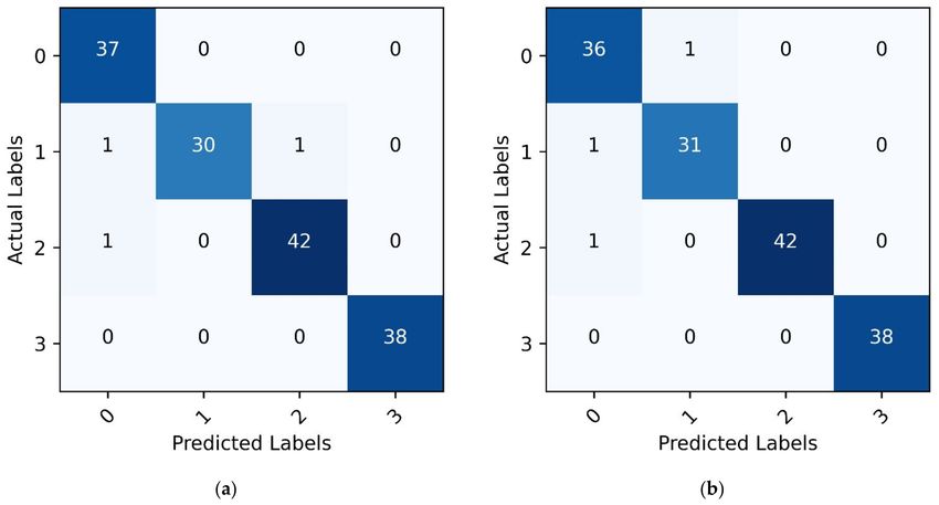
Sensors 2021, 21, 4716                                                                                           4 of 17

                         connecting the anaerobic digester to the energy recovery section. The samples of Class
                         0 were collected in the WWTP area, taking care that the air at the moment of sampling
                         was not affected by the odor sources considered in the study; however, as a result of the
                         proximity of another industrial wastewater treatment plant, it was not always possible to
                         sample odorless air. In Figure 1, the locations of the sampling points are defined.
                              Air samples were collected in accordance with EN 13725:2003, where Nalophan®
                         sampling bags with an 8 L volume were used; the samples with higher concentrations were
                         diluted to 1:10 to increase the dataset size with a predilution system: model EPD10000
                         (Olfasense GmbH, Kiel, Germany). The IOMS (MSEM32® by Sensigent, Baldwin Park, CA,
                         USA) was located in position 9 (Figure 1), near the fenceline of the plant along the direction
                         of prevailing winds coming from the plant to the nearest urban receptors. After collection
                         in duplicates, each sample was fed to the IOMS on the same day, and the twin sample
                         was analyzed using dynamic olfactometry (DO) at the T&A Laboratory within 24 h, using
                         the LEO dynamic olfactometer (ARCO Solutions srl, Trieste, Italy) for the measurement of
                         Odor Concentrations (Cod), which are expressed as European odor unit (ouE/m3 ). A total
                         of 51 samples were collected, with odor concentrations ranging from 20 to 2435 ouE/m3 .

                         2.2. Experimental Protocol for Data Acquisition
                               The dataset used for ML application was collected by an IOMS with an array of 32
                         sensors (S3, S4, S5 Environmental Sensors, i.e., pressure, humidity, and temperature, S7, S8,
                         S9, S10 Electrochemical Sensors, S11-12-13-14 Metal Oxide Sensors, S18 Photoionization De-
                         tector, S21-22-23-24 Nanocomposite-based Sensors, S42-43-44-45-46-47-48-49 Metal Oxide
                         Sensors, S50-51-52-53-54-55 Nanocomposite-based Sensors, S56-57 Metal Oxide Sensors).
                         The instrument was equipped with a cartridge filter to obtain odorless air (zero air-ZA): air
                         was drawn by the instrument after filtering to remove odorous compounds but preserve
                         the temperature and humidity of the ambient air. The training phase was carried out in
                         the field, as it is important that the samples were fed in different environmental conditions
                         (humidity and temperature) [34], as variations in temperature and humidity may signifi-
                         cantly influence the baseline of resistance of the sensors [35,36] and, consequently, affect
                         the calculations of the sensor responses. In order to ensure that the baseline before sample
                         feeding represented the ambient air conditions of odorless air, ZA was drawn in by the
                         instrument. Moreover, a certain amount of time elapsed before the following feeding so
                         that the sensors returned to the baseline values. Consequently, the measurement cycle
                         consisted of 1 min of ZA, 2 min sample draw-in by IOMS (acquisition phase), and 3 min for
                         baseline recovery; for each sample, the measurement cycle was repeated four times. The
                         duration of each phase was determined on the basis of the literature [13] and observing
                         the response of the sensors in terms of the time required to reach a steady state value
                         during the feeding of the samples, which was less than 90 s (see Section 2.3). The sampling
                         frequency of the instrument was set to 0.1 Hz, so that 12 data points were available for each
                         sample replicate.

                         2.3. Data Pretreatment
                              All data collected by the IOMS, representing the sensor responses, were stored in a
                         secure cloud storage and then extracted for elaboration. In Figure 2, the selected sensor
                         responses during the four measurement cycles of one sample are shown, in which a simple
                         zero normalization was applied to the process data for better visualization.
                              Data smoothing using low-pass digital filters was useful to clean up the signals and
                         better identify the response of the sensors. A Savitzky–Golay filter based on least-squares
                         smoothing with a polynomial order of 3 was used to filter the data, as this algorithm
                         reduces the noise while maintaining the shape and height of the original signal [37,38].
                         Then, the response curves, representing the dynamic variation in the electrical resistance
                         of the sensors [39], were analyzed to extract piecemeal signal features. Although several
                         features are extractable from the response curves (steady-state response, rising time, falling
                         time) [12], recent studies suggest that the peak values of the signals, representing the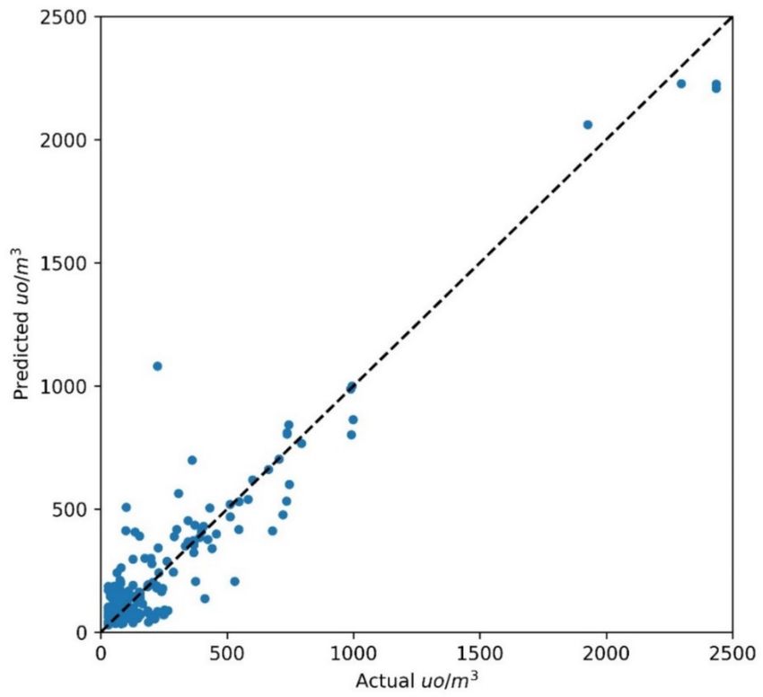
Sensors 2021, 21, 4716                                                                                                        5 of 17

                                   maximum degree of change in the sensors responding to odor, are more effective for odor
                                   classification [13].

                                   Figure 2. Measurements cycles during sample feeding.

                                       Consequently, for the sensor i, the fractional difference xi in the signal relative to the
                                   peak values was used [12,13], by considering the associated piecemeal signal within the
                                   2-min acquisition phase:
                                                                    xi = Ri − Rbl,i /Rbl,i                                     (1)
                                   where Ri is the resistance peak value after feeding and Rbl,i is the baseline resistance, as
                                   detected during the zero-air drawn-in cycle, for the sensor i. At present, we do not have
                                   sufficient information to confirm whether the response of the sensors that gave a positive
                                   response (nanocomposite-based sensors) varies with the variation in chemical species and,
                                   therefore, whether this information can be used in ML algorithms. Consequently, we used
                                   the variation in the absolute value of the sensor values from the baseline. The duration of
                                   the peak phase varies as a function of sample concentrations, ranging from 1 min to 80 s,
                                   so that 6–8 data points were considered for each measurement cycle.
                                        In Table 1, the characteristics of the resulting dataset are shown.

              Table 1. Structure of the dataset used, divided by odor classes and indicating the odor concentrations range.

            Classes                 Number of Samples 1                     Number of Data         Concentrations Range [ouE/m3 ]
             Class 0                           28                                     216                       20–200
             Class 1                           24                                     160                      25–2435
             Class 2                           28                                     214                       40–510
             Class 3                           24                                     160                      64–1866
                                                          1   Including replicates.

                                        The averages and standard deviations for each class are 44 ouE/m3 and 36 ouE/m3 ,
                                   for Class 0; 518 ouE/m3 and 517 ouE/m3 , for Class 1; 184 ouE/m3 and 169 ouE/m3 , for
                                   Class 2; and 416 ouE/m3 and 331 ouE/m3 , for Class 3.

                                   2.4. Algorithms for Odor Classification and Regression
                                         MATLAB R2017b (MathWorks, Natick, MA, USA) and Python 3.7 with the packages
                                   scikit-learn 0.23 (https://scikit-learn.org/stable/ (accessed on 24 March 2021)) and Keras
                                   2.4 (https://keras.io (accessed on 14 April 2021)) were used for data pretreatment, feature
                                   extraction, and model selection. In particular, Keras 2.4 was employed for the MLP model,
                                   whereas scikit-learn was used for Random Forest.
Sensors 2021, 21, 4716                                                                                           6 of 17

                         2.4.1. Feature Extraction and General Workflow
                              In Figure 3, the overall workflow for model development is given. After data pre-
                         treatment, several tests were carried out to choose an appropriate subset of the input
                         variables—the 32 values of fractional difference xi —using the Recursive Feature Elimi-
                         nation algorithm with cross-validation (RFECV) [40], such that only the most significant
                         sensors were employed for the specific case. RFECV was employed for both the classifica-
                         tion and the regression task.

                         Figure 3. Workflow of model development for the classification and regression tasks.

                               The overall dataset with the selected features was split into a training and test set
                         according to the ratio 80:20, so that 600 data points were used for training and 150 were
                         used for testing.
                               Cross-validation allows one to check for overfitting and is particularly useful when
                         dealing with MLP. A fivefold cross-validation approach was employed for the selected
                         model: at every iteration, the training set (600 data points) was split into five, with one
                         portion being kept as the validation set to test the performance with the trained parameters.
                               After the cross-validation and selection of the model, the last step was to use the test
                         set (20% of the dataset) to analyze the performances of the selected models for classification
                         and regression problems.
                               For the classification task, a confusion matrix CM was calculated for MLP and RF, and
                         the related scoring parameters were calculated, such as the classification accuracy rate for
                         each class (aci ) and the overall accuracy rate (aco ):
                                                                            cmii
                                                       aci =                                                        (2)
                                                               cmii + ∑k6=i cmik + ∑ j6=i cm ji

                                                                           ∑i cmii
                                                                   aco =                                            (3)
                                                                           ∑i,j cmij
                         where cmij are the components of the confusion matrix CM.
                             Moreover, as we were dealing with a multiclassification problem with potentially
                         unbalanced classes—in which Class 0 would be more frequent during real-time acquisition—
                         Cohen’s kappa was used as a score parameter to compare the classification accuracy of the
                         models [41]:
                                                                Pr ( a) − Pr (e)
                                                            k=                                                  (4)
                                                                  1 − Pr (e)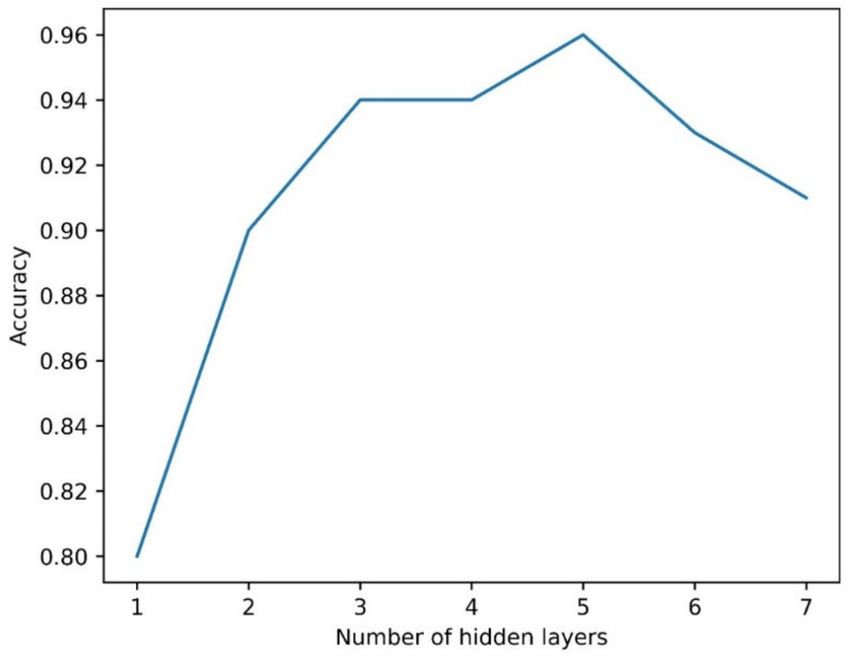
Sensors 2021, 21, 4716                                                                                            7 of 17

                         where Pr ( a) is the probability of agreement, while Pr (e) is the measure of the agreement
                         between the model predictions and the actual class values as if happening by chance. The
                         introduction of this parameter is related to the predicted field applications of the IOMS. If,
                         for example, after a monitoring campaign lasting a time T, it turns out that the classification
                         gives 90% of T for Class 0 and 10% of T of Class 1, and we are interested in comparing the
                         predicted classes with the actual ones, using the overall accuracy rate aco would distort the
                         result, as it does not take into account that the classes are unbalanced.
                              Therefore, Cohen’s kappa is used to deal with such situations, which will most likely
                         occur during field monitoring. Furthermore, as Cohen’s kappa exploits the Expected
                         Accuracy, namely, a measure representing the dependence obtained by chance between
                         the predicted and the true classification measure [42], this allows for the comparison of
                         different models, which was one of the goals of the paper.
                              For regression task, the coefficient of determination (R2 ), and the root mean square
                         error (RMSE) were calculated, which is discussed in Section 3.3.

                         2.4.2. Artificial Neural Network
                              In the present work, a feed forward neural network or Multilayer Perceptron (MLP)
                         was employed [43]. ANN models have two contour layers: a first layer or input layer in
                         which the features selected by the RFECV are introduced, and an output layer in which
                         the predicted values are generated: target outputs were the four odor classes for the
                         classification problem and the odor concentrations for the regression. Between these
                         two layers exist one or more layers called hidden layer or layers: when more than one
                         hidden layer is employed, the learning process of neural networks is defined as deep
                         learning. During the neural training phase, different parameters minimize the errors
                         between the input and the predicted variable. To find the best model, it is necessary to
                         use the trial-and-error approach through which different topologies are analyzed. The
                         number of hidden layers and the number of neurons for each layer were selected using the
                         following procedure:
                         •    First, a single hidden layer was employed, the accuracy was calculated, and then other
                              layers were added until the appropriate accuracy was obtained;
                         •    In order to further increase the accuracy, an increasing number of neurons per layer
                              was tested, starting from 10.
                               The hidden layer activation function selected was ReLU as a result of its speed in
                         training. The sotftmax output layer activation function was chosen for classification, re-
                         stricting the output of the model to the range (0,1), while the linear function was chosen
                         for regression.
                               Two kinds of loss functions for classification and regression were tested, namely,
                         categorical cross entropy and mean squared error. Categorical cross-entropy loss [44]
                         measures the performance of a classification model whose output is a probability value
                         between 0 and 1, as given by the softmax function of the output layer. Cross-entropy loss
                         increases as the predicted probability diverges from the actual label, while, on the other
                         hand, a perfect model would have a log cross-entropy loss of 0. Categorical cross-entropy
                         can be used for the classification task but not for regression. On the other hand, mean
                         squared error (MSE) as the loss function can used for both classification and regression;
                         thus, it was chosen after some preliminary tests.

                         2.4.3. Random Forest
                              RF is a supervised learning model, i.e., it is an evolution of decision tree learning
                         in which each node focuses on a certain attribute of the data and determines what class
                         (classification) or value (regression) the data are most likely to have [45]. RF was recently
                         employed for odor classification to evaluate product quality [20,46], while no applications
                         for environmental monitoring of odor emissions are known to date; hence, a detailed
                         discussion on the algorithm and its genesis is provided below.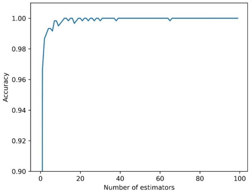
Sensors 2021, 21, 4716                                                                                            8 of 17

                               A decision tree consists of a collection of nodes, divided into root nodes, decision
                         nodes, and leaf nodes. The training dataset is passed from the root to leaves, and for each
                         node, there are splitting rules for one specific feature. The goal of each split in a decision
                         tree is to move from a confused dataset to two (or more) purer subsets.
                               Entropy can be used to measure information disorder. In a classification problem, if
                         we have a dataset with S elements divided in k classes, the frequency pi of a class i in the
                         dataset is given by Si /S, where Si is the number of elements belonging to the class i. Then,
                         the information entropy Hs is defined as follows:

                                                                        k
                                                              Hs := − ∑ pi log2 pi .                                 (5)
                                                                       i =1

                              It can be observed that entropy is minimum (= 0) if all the elements of S belong to
                         the same class i, and is maximum (= log2 k) if all the k classes are represented in S by the
                         same number of elements. In order to measure how good a split in a decision tree is, one
                         parameter that can be adopted is the Information Gain (IG), which represents the difference
                         in entropy before and after the split and is defined as
                                                                               r
                                                             IG := Hs −       ∑ p j Hsj                              (6)
                                                                              j =1

                         where the first term is the entropy before the split, the second term is the entropy after the
                         split, calculated as the sum of the entropy of each j class of the r subclasses generated by
                         the split, weighted on the frequency pj of a class j. Consequently, at each step, the data are
                         split in a way to obtain the highest value in IG, as this leads to the purest subsets.
                               The aforementioned definitions were clearly developed for the classification tasks,
                         where entropy measures the quality of the correct attribution of an element in the appro-
                         priate category or class. For regression, the goal of the RF (as in all the ML methods) is to
                         optimize the prediction error, in the form of Mean Squared Error. Such concepts, initially
                         developed for decision tree learning, are the same in RF, which is a model that takes into
                         account multiple decision tree models developed from random subsets of the training data.
                         Bootstrap is the technique that involves random sampling of small subset of data from the
                         training dataset. In comparison with a single decision tree, an RF model achieves better
                         precision values. The way in which the multiple randomly selected decision trees cooperate
                         to give the predictions is called bootstrap aggregation or bagging. Bagging is an ensemble
                         technique that is used to reduce the variance of the prediction model by combining the
                         results of multiple decision trees modeled on different subsets of instances of the dataset.
                         During classification or regression on new data, each tree “votes” by contributing its own
                         prediction to the ensemble’s final prediction; in classification, the class with the most votes
                         is the final prediction, whereas the ensemble average of the trees is the final prediction for
                         regression. The number of trees employed in RF is usually called the number of estimators.
                               To find the best RF model, the following procedure was adopted: the accuracies for
                         different random forests were calculated with a number of trees (estimators) between 1
                         and 100, and the RF structure that obtained the best accuracy was chosen.

                         3. Results and Discussion
                         3.1. Feature Selection
                              In order to select the independent variables that best reflect the input and output
                         relationship and remove the redundant independent variables, the Recursive Feature
                         Elimination algorithm with cross-validation (RFECV) was adopted for selecting a subset
                         of the 32 values of fractional difference xi , which was used as input to the models. It was
                         decided to use features that were between rank 1 and rank 8 of the RFECV algorithm to have
                         a balance between the number of selected features, which we set to 12. Features selected
                         for classification based off the RFECV ranking were the following sensors: S13 (MOS),
Sensors 2021, 21, 4716 9 of 17
S21 (NCA), S24 (NCA), S44 (MOS), S46 (MOS), S7 (EC), S57 (MOS), S54 (NCA), S11 (MOS),
S42 (MOS), S23 (NCA), and S9 (EC). Features selected for regression based off the RFECV
ranking were the following sensors: S12 (MOS), S5 (AS), S55 (NCA), S11 (MOS), S49
(MOS), S47 (MOS), S7 (EC), S10 (EC), S4 (AS), S51 (NCA), S13 (MOS), and S23 (NCA).
As a result of the nature of the RFECV algorithm, it is not straightforward to explain the
differences in the lists between classification and regression. However, it can be pointed
out that Environmental sensors S5 and S4 were relevant when the regression task was to
be carried out by the IOMS, while it appears that classification was not affected by such
conditions. This observation is consistent with the literature [13], wherein classification was
carried out using 13 MOS chemical sensors (MOS), without taking into account the three
environmental sensors; however, more recent findings [47] suggest that the temperature of
the gaseous flux in the measurement chamber can be considered as a relevant feature in
order to increase the overall classification accuracy (from 96% to 98%).
3.2. Classification
The hyperparameters of the ML models were selected for the classification task and
are represented by the number of hidden layers and the node for MLP and the number of
decision trees or estimators for Random Forest. It was decided to increase the number of
hidden layers, varying them between 1 and 7, with an initial number of neurons equal to
10. As highlighted in Figure 4, the maximum accuracy for MLP was achieved with five
hidden layers.
Figure 4. MLP: accuracy in relation to the number of hidden layers.
After selecting the number of hidden layers, a trial-and-error approach was used
to select the number of neurons per layer, starting from 10. The best results in terms of
accuracy were obtained with 100 neurons.
The classification task with RF was first carried out by selecting the hyperparameter
of the model, namely, the number of estimators. As can be seen from Figure 5, the accuracy
value for RF rapidly increased and stabilized when more than five estimators were used;
thus, 20 estimators were chosen.
Once the models (MLP and RF) were selected, the classification accuracy rates for
each class and the overall accuracy rate were calculated for the best models. The results for
the training set are shown in Table 2.Sensors 2021, 21, 4716 10 of 17
Figure 5. Accuracy in relation to the number of estimators (trees) for Random Forest.
Table 2. Classification accuracy rates for each class and the overall accuracy rates for MLP and RF
with the training dataset.
Classes MLP RF
Class 0 0.99 1
Class 1 0.99 1
Class 2 1 1
Class 3 1 1
Overall 0.99 1
It is not unusual for such high values to occur when testing a model on the training
set. To find out if there was an overfitting problem, and consequent poor predictive
performances on new data, 5-fold cross-validation (CV) was adopted, which has not been
applied thus far in papers dealing with IOMS classification or regression applications in
complex field situations. In detail, the overall accuracy rate of MLP and RF was calculated
five consecutive times by splitting the training dataset (600 data) into internal training data
(480 data points) and validation data (120 data points) with different splits each time. The
models were fitted on internal training data, and the scores were computed with reference
to validation data.
Table 3 presents the overall classification accuracies as the scores of the models calcu-
lated for each split and the mean cross-validation (CV) score and the associated standard
deviation. Low standard deviations indicate that the choice of training data did not affect
the overall classification accuracy, thus indicating that overfitting was avoided.
Table 3. Five-fold cross-validation results.
Overall Classification Accuracy
MLP RF
First Split 0.95 0.97
Second Split 0.98 0.98
Third Split 0.97 0.97
Fourth Split 0.98 0.99
Fifth Split 0.97 0.97
Mean CV Score 0.97 0.98
Standard Deviation CV Score 0.05 0.03Sensors 2021, 21, 4716 11 of 17
Then, the prediction capability of the selected models was evaluated with the test
dataset. The goodness of the classification can be examined through the construction of
a confusion matrix through which we observe which odor classes have been correctly
classified and to what quantity. Each row of the matrix represents the instances in an actual
class, while each column represents the instances that the classifier assigns.
Figure 6 shows the confusion matrix obtained by MLP and Random Forest for the
test dataset.
Figure 6. Confusion matrix for the test dataset with two classification algorithms: (a) MLP; (b) Random Forest.
As regards the overall result, it can be seen that only three elements out of 150 were
mismatched for both MLP and RF. By constructing the confusion matrix, the classification
accuracy rates, the overall accuracy rate, and Cohen’s kappa can be easily calculated, as
Pr ( a) is given by the sum of the diagonal elements in the confusion matrix divided by
the total, whereas the Pr (e) definition is more complex, but it can be recovered from the
components of the confusion matrix.
In Table 4, the aforementioned classification metrics are shown for the test dataset. The
Cohen’s kappa coefficient, which is used in the present paper as a suitable score parameter
for multiclass classification, is 97% for RF and MLP.
Table 4. Classification accuracy rates for each class, overall accuracy rates, and Cohen’s kappa for
MLP and RF with the test dataset.
Classes MLP RF
Class 0 0.98 0.97
Class 1 0.98 0.98
Class 2 0.98 0.99
Class 3 1 1
Overall Accuracy Rate 0.98 0.98
Cohen’s Kappa 0.97 0.97
Apart from the overall accuracy rates, it is interesting to highlight the classification
rate for Class 0, which represents ambient air without the influence of odor emissions from
the three sources considered in the study, i.e., pretreatments (Class 1), sludge conditioningSensors 2021, 21, 4716 12 of 17
(Class 2), and biogas from anaerobic digestion (Class 3). No difference was observed in the
classification accuracy rate between Class 0 and the other classes.
In a recent IOMS field application, misclassification of ambient air was found for both
the algorithms employed (Linear Discriminant Analysis and ANN), which were not able to
identify this class in any case. It was suggested that this was because the sensors were more
sensitive to odorous classes [13]. In the present case, ANN performed reasonably well for
Class 0, giving a specific classification accuracy of 98% for this class, as compared to poor
values obtained in [13], in which one hidden layer was chosen, as opposed to five in the
present work. The divergence can be partially attributed to the different models, as in the
last few years, it was recognized that a deeper model provides a hierarchy of layers that
builds up increasing levels of abstraction from the space of the input variables to the output
variables, thus suggesting that using deep architectures expresses a useful prior over the
space functions the model learns [48]. Furthermore, RF also performed well for Class 0,
so that the significant difference in the classification accuracy rate might be related to the
different characteristics of the ambient air, which, in our case, was not totally odorless as a
result of the presence of another wastewater treatment plant close by, emitting odorous
compounds very different from the investigated classes. It is probable that the presence of
other external sources in the ambient air was helpful for better discriminating the WWTP
sources. This hypothesis could have been tested by sampling the odor emissions of the
outer sources, but unfortunately, this was not possible. Access to each emission source,
in fact, is essential to ascertain whether the Class 0 detections (not recognized) refer to
emissions from another source or to ambient odorless air. This must be taken into account
when IOMS are to be installed outside the fenceline of industrial emission sources, when
they are not available for sampling. In other words, the current state of knowledge suggests
that is not meaningful to use an IOMS for classification when all the relevant odor emission
sources are not sampled and used for training.
3.3. Regression
First, the results obtained on the training set are discussed; then, the results from
the 5-fold cross-validation and the performance of the models measured on the test set
are shown. For odor concentration regression, we chose the same MLP structure as the
classification, and the associated results turned out to be satisfying. Table 5 shows the
coefficient of determination (R2 ) and root mean squared error (RMSE) for both models
based on the training dataset. We also attempted to reduce the number of hidden layers and
neurons to obtain a simpler network, but this only led to a loss of performance similar to
that seen in classification (Figure 4), with no significant decrease in terms of computational
time; thus, there was no advantage in changing network hyperparameters.
Table 5. Regression coefficients and root mean square error for MLP, RF, and ANN developed in [30],
based on the training dataset.
Classes MLP RF ANN [30]
R2 0.99 0.99 0.9976
RMSE (ouE/m3 ) 36.9 6.8 523,4
NRMSE (%) 1.52 0.28 1.05
Both algorithms were found to be very precise on the training set with equal R2 . In
a similar case concerning odor emissions from WWTP [30], a similar value of R2 (0.996)
was found for the training set, with an ANN model (13 nodes for input layer, one hidden
layer, with eight neurons) developed on data provided by seedOA IOMS [13]. RMSE was
equal to 36.9 ouE/m3 for MLP and 6.8 ouE/m3 for RF, so that RF may be considered more
accurate than MLP, based on the training dataset.
Keeping in mind the results of [30], a straightforward comparison of the RMSE is not
possible, as the dependent variable (odor concentration) ranged from 20 to 2435 ouE/m3 in
our case, while it varied from 20 to 50,000 ouE/m3 in [30]. By normalizing the RMSE usingSensors 2021, 21, 4716 13 of 17
the difference between the maximum (ymax ) and minimum (ymin ) of the training dataset
(NRMSE = RMSE/(ymax − ymin )), we obtained similar results for MLP and ANN in [30],
with an NRMSE between 1.05% and 1.52%, while RF demonstrated an NRMSE of 0.28%.
For the regression task, 5-fold cross-validation was also adopted to control whether
the proposed models were overfitted and then could have poor predictive performance on
new data. The mean CV score (R2 ) and standard deviation CV score for the models were
0.9 and 0.008 for MLP and 0.95 and 0.029 for RF, respectively. Low standard deviations for
the cross-validation scores for both models suggest that overfitting was avoided and the
models could be used for prediction on the test set. In Figure 7, the correlation between the
odor concentrations measured using dynamic olfactometry for the test set (150 data points)
and the values predicted by MLP is shown.
Figure 7. Actual and predicted values of odor concentration (ou/m3 ) obtained with MLP on the
test set.
The coefficient of determination on the test set was 0.9, while the RMSE was 130 ouE/m3 ,
which is greater than the RMSE calculated on the training set (36.9 ouE/m3 ). The NRMSE
for MLP on the test data was 5.37%, which can be considered satisfying if we consider the
uncertainty associated with measures with dynamic olfactometry [49]. The Random Forest
model demonstrated comparable or slightly better results than MLP on the training set,
and this was confirmed for the test set, as indicated in Figure 8.
The coefficient of determination on the test set was 0.92, while the RMSE was 97 ouE/m3 :
ten times greater than the RMSE calculated on the training set. Unfortunately, no perfor-
mance indicators on the test set are available from [30], so that in Table 6, a straightforward
comparison between the models is only possible for those proposed in the present work.Sensors 2021, 21, 4716 14 of 17
Figure 8. Actual and predicted values of odor concentration (ou/m3 ) obtained with RF on the test set.
Table 6. Regression coefficients and root mean square error for MLP and RF based on the test dataset.
Classes MLP RF
R2 0.9 0.92
RMSE (ouE/m3 ) 130 97
NRMSE (%) 5.37 4.02
While the two different algorithms, i.e., MLP and RF, exhibited almost the same
performance for the classification, for the regression, we obtained slightly different values,
which may be due to several factors. These include the difference between the RF classifier
and RF regressor, the different features selected by the feature selection algorithm for
classification and regression, and the different types of targets for regression (continuous
variable) and classification (discrete variable). Although the NRMSE for RF on the test
data was 4%, indicating a better overall performance than MLP, it must be pointed out
that the incremental ratio in the RMSE between the training set and test set was 3.5,
whereas a 14-fold increase was observed when comparing the RMSE for the training set
(6.8 ouE/m3 ) and the test set (97 ouE/m3 ) for RF. Collecting more samples from different
WWTP plants [29] in order to increase the size of the dataset will be a valuable approach to
confirm the discrepancy between the RMSE in the training set and test set and whether the
NRMSE from the test set is below 10%. These can be considered good results for reliable
continuous fenceline monitoring of odor emissions.
The results show that it is possible, even for complex situations, to develop field
instrumental odor monitoring applications enhanced by ML algorithms, which are capa-
ble of simultaneously performing classification and regression, with interesting practical
applications. In fact, it is thought that the dissemination of detailed knowledge concern-
ing algorithms and their performance in the environmental monitoring of odors, with
transparent protocols useful for verifying their performance, will make policy makers
and environmental protection agencies increasingly inclined to set odor thresholds at
plant fencelines [33] and evaluate these values in a monitoring campaign. This has al-Sensors 2021, 21, 4716 15 of 17
ready happened in recent years [21,22,28,29] due to growing pressure from the public
and citizens’ complaints. In such a rapidly evolving context, it may be useful to carry
out classification and regression simultaneously from both the plant operator’s and the
Environmental Protection Agency’s point of view. When fence monitoring with IOMS is
mandatory or strongly encouraged, plant operators will be interested in establishing the
source of odor emission within a plant that is responsible for the highest concentrations
detected at the fenceline, especially when the sources cannot be directly monitored, as in
the case of fugitive emissions. If, on the other hand, the Environmental Protection Agency
is requested to identify the most critical emission sources from one or more plants located
nearby, concentration alone or odor class alone is insufficient to carry out this task; i.e.,
both odor concentration and class are essential to tackle such complex tasks.
In the present case study, it may be necessary to establish the distribution of odor
classes (0, 1, 2, 3) within a specific concentration range. If odor Class 0 (ambient air) is
more frequent at low odor concentrations, this odor class is going to be associated with
clean background air, while if odor Class 0 is more frequent at high concentrations, another
source will be responsible for high odor concentrations. This source may have come be
from outside the plant, having not been identified during IOMS training. The monitoring
campaign to be carried out in the WWTP of Monopoli will address such issues. Although
it is not possible to carry out classification when all odor emission sources are not used for
training (Section 3.2), the joint analysis of concentrations and odor classes could provide
useful information on complex multisource odor emission problems.
4. Conclusions
The paper describes the employment of two machine learning algorithms (Multilayer
Perceptron and Random Forest) to elaborate signals acquired from a commercial IOMS
used for fenceline odor monitoring at an urban wastewater treatment plant, in order to
develop concurrent odor classification and regression models.
As for classification with multiple odor classes, Cohen’s kappa was used as the score
parameter to measure the performances of the algorithms on the test set, yielding 97% for
both models. For odor concentration regression, NRMSE was used as the performance
parameter by normalizing RMSE using the difference between the maximum and minimum
of the odor concentrations range. This was done in order to obtain a performance parameter
useful for directly comparing the accuracies of IOMSs, even those operating in real cases
with different odor emission intensities.
The research aimed to support machine learning applied to environmental odor
monitoring with IOMS. In the near future, low-cost sensors using specific performance
factors (Cohen’s kappa for classification and NRMSE for regression) will facilitate the
use of such systems in the environmental monitoring sector and ensure the possibility of
performance comparison between different IOMS.
Author Contributions: Conceptualization, F.C.; methodology, F.C., E.B.; software, E.B.; data gather-
ing and experiments, G.D.S.; writing, F.C.; research administration, F.C.; Funding Acquisition, F.C.
All authors have read and agreed to the published version of the manuscript.
Funding: This research was supported by Regione Puglia, under “Progetto ASPIDI”, grant number
B31B19001170007 and the APC was funded by T&A.
Institutional Review Board Statement: Not applicable.
Informed Consent Statement: Not applicable.
Data Availability Statement: Data available on request due to restrictions.
Acknowledgments: AQP SpA and LabService Analytica srl are acknowledged for their technical support.
Conflicts of Interest: The authors declare no conflict of interest.Sensors 2021, 21, 4716 16 of 17
References
1. Hayes, J.E.; Stevenson, R.J.; Stuetz, R.M. The impact of malodour on communities: A review of assessment techniques. Sci. Total
Environ. 2014, 500, 395–407. [CrossRef]
2. Bokowa, A.; Diaz, C.; Koziel, J.A.; McGinley, M.; Barclay, J.; Schauberger, G.; Guillot, J.-M.; Sneath, R.; Capelli, L.; Zorich, V.; et al.
Summary and overview of the odour regulations worldwide. Atmosphere 2021, 12, 206. [CrossRef]
3. General Determinations Regarding the Characterization of Atmospheric Emissions from Activities with a High Odour Impact,
D.g.r. 15 February 2012–n. IX/3018. Available online: http://www.olfattometria.com/download/dgr-lomb.pdf (accessed on
2 July 2021).
4. Law on Odour Emissions. L.R. 16 July 2018–n. 32. Available online: http://www.ager.puglia.it/documents/10192/29519220
/LR_32_2018.pdf (accessed on 2 July 2021).
5. Brattoli, M.; Mazzone, A.; Giua, R.; Assennato, G.; de Gennaro, G. Automated Collection of Real-Time Alerts of Citizens as a
Useful Tool to Continuously Monitor Malodorous Emissions. Int. J. Environ. Res. Pub. Health 2016, 13, 263. [CrossRef]
6. Real Time, Automatic and Remote-Activated Sampling System for Industrial Odour Emissions Compliant with the Euro-
pean Standard EN 13725, CORDIS EU Research Results. Available online: cordis.europa.eu/project/id/756865 (accessed on
2 July 2021).
7. Lotesoriere, B.; Giacomello, A.; Bax, C.; Capelli, L. The Italian Pilot Study of the D-NOSES Project: An Integrated Approach
Involving Citizen Science and Olfactometry to Identify Odour Sources in the Area of Castellanza (VA). Chem. Eng. Trans. 2021,
85, 145–150.
8. Karakaya, D.; Ulucan, O.; Turkan, M. Electronic Nose and Its Applications: A Survey. Int. J. Aut. Comp. 2020, 17, 179–209.
[CrossRef]
9. Stuetz, R.M.; Fenner, R.A.; Engin, G. Assessment of odours from sewage treatment works by an electronic nose, H2 S analyzer and
olfactometry. Water Res. 1999, 33, 453–461. [CrossRef]
10. Qu, G.; Omotoso, M.M.; el-Din, M.G.; Feddes, J.J.R. Development of an integrated sensor to measure odors. Environ. Monit.
Assess. 2008, 144, 277–283. [CrossRef]
11. Bax, C.; Sironi, S.; Capelli, L. How Can Odors Be Measured? An Overview of Methods and Their Applications. Atmosphere 2020,
11, 92. [CrossRef]
12. Yan, J.; Guo, X.; Duan, S.; Jia, P.; Wang, L.; Peng, C.; Zhang, S. Electronic Nose Feature Extraction Methods: A Review. Sensors
2015, 15, 27804–27831. [CrossRef] [PubMed]
13. Zarra, T.; Galang, M.G.K.; Ballesteros, F.C., Jr.; Belgiorno, V.; Naddeo, V. Instrumental Odour Monitoring System Classification
Performance Optimization by Analysis of Different Pattern-Recognition and Feature Extraction Techniques. Sensors 2021, 21, 114.
[CrossRef]
14. Vanarse, A.; Espinosa-Ramos, J.I.; Osseiran, A.; Rassau, A.; Kasabov, N. Application of a Brain-Inspired Spiking Neural Network
Architecture to Odor Data Classification. Sensors 2020, 20, 2756. [CrossRef] [PubMed]
15. Wen, T.; Mo, Z.; Li, J.; Liu, Q.; Wu, L.; Luo, D. An Odor Labeling Convolutional Encoder–Decoder for Odor Sensing in Machine
Olfaction. Sensors 2021, 21, 388. [CrossRef]
16. Yan, L.; Wu, C.; Liu, J. Visual Analysis of Odor Interaction Based on Support Vector Regression Method. Sensors 2020, 20, 1707.
[CrossRef]
17. Misselbrook, T.H.; Hobbs, P.J.; Persaud, K.C. Use of an Electronic Nose to Measure Odour Concentration Following Application
of Cattle Slurry to Grassland. J. Agric. Eng. Res. 1997, 66, 213–220. [CrossRef]
18. Aguilera, T.; Lozano, J.; Paredes, J.; Álvarez, F.; Suárez, J. Electronic nose based on independent component analysis combined
with partial least squares and artificial neural networks for wine prediction. Sensors 2012, 12, 8055–8072. [CrossRef]
19. Zhang, L.; Tian, F.; Nie, H.; Dang, L.; Li, G.; Ye, Q.; Kadri, C. Classification of multiple indoor air contaminants by an electronic
nose and a hybrid support vector machine. Sens. Actuators B Chem. 2012, 174, 114–125. [CrossRef]
20. Men, H.; Fu, S.; Yang, J.; Cheng, M.; Shi, Y.; Liu, J. Comparison of SVM, RF and ELM on an Electronic Nose for the Intelligent
Evaluation of Paraffin Samples. Sensors 2018, 18, 285. [CrossRef] [PubMed]
21. Cangialosi, F.; Intini, G.; Colucci, D. On Line Monitoring of Odour Nuisance at a Sanitary Landfill for Non-Hazardous Waste.
Chem. Eng. Trans. 2018, 68, 127–132.
22. Bax, C.; Lotesoriere, B.; Capelli, L. Real-time Monitoring of Odour Concentration at a Landfill Fenceline: Performance Verification
in the Field. Chem. Eng. Trans. 2021, 85, 19–24.
23. Cangialosi, F. Advanced Data Mining for Odour Emissions Monitoring: Experimental Peak-to-mean Calculations and Spectral
Analysis of Data Derived from Ioms in two waste Treatment Plants. Chem. Eng. Trans. 2021, 85, 7–12.
24. Majchrzak, T.; Wojnowski, W.; Dymerski, T.; G˛ebicki, J.; Namieśnik, J. Electronic noses in classification and quality control of
edible oils: A review. Food Chem. 2018, 246, 192–201. [CrossRef]
25. Tan, J.; Xu, J. Applications of electronic nose (e-nose) and electronic tongue (e-tongue) in food quality-related properties
determination: A. review. Artific. Intell. Agric. 2020, 4, 104–105. [CrossRef]
26. Wijaya, D.R.; Sarno, R.; Zulaika, E. DWTLSTM for electronic nose signal processing in beef quality monitoring. Sens. Actuators B
Chem. 2021, 326. [CrossRef]
27. Bax, C.; Sironi, S.; Capelli, L. Definition and Application of a Protocol for Electronic Nose Field Performance Testing: Example of
Odor Monitoring from a Tire Storage Area. Atmosphere 2020, 11, 426. [CrossRef]Sensors 2021, 21, 4716 17 of 17
28. Oliva, G.; Zarra, T.; Pittoni, V.; Senatore, V.; Galang, M.G.M.; Castellani, M.; Belgiorno, V.; Naddeo, V. Next-generation of
instrumental odour monitoring system (IOMS) for the gaseous emissions control in complex industrial plants. Chemosphere 2021,
271, 129768. [CrossRef] [PubMed]
29. Research Project ASPIDI. Available online: https://www.progettoaspidi.com (accessed on 2 June 2021).
30. Galang, M.G.; Zarra, T.; Naddeo, V.; Belgiorno, V.; Ballesteros, F.C., Jr. Artificial Neural Network in the Measurement of
Environmental Odours by E-Nose. Chem. Eng. Trans. 2018, 68, 247–252.
31. Zarra, T.; Galang, M.G.; Ballesteros, F.; Naddeo, V.; Belgiorno, V. Environmental odour management by artificial neural network—
A review. Environ. Int. 2019, 133, 105189. [CrossRef]
32. Naddeo, V.; Zarra, T.; Oliva, G.; Kubo, A.; Ukida, N.; Higuchi, T. Odour measurement in wastewater treatment plant by a new
prototype of e.Nose: Correlation and comparison study with reference to both European and Japanese approaches. Chem. Eng.
Trans. 2016, 54, 85–90.
33. Guidelines for Issuing Technical Opinions Regarding the Emissions into Atmosphere Produced by Wastewater Treatment Plant.
ARPA Puglia (rev. 2014). Available online: https://old.arpa.puglia.it/c/document_library/get_file?uuid=6e747fc8-859a-4cd6-9
302-bb73913f7410&groupId=13879 (accessed on 2 June 2021).
34. UNI 11761:2019; Emissioni e Qualità Dell’aria-Determinazione Degli Odori Tramite IOMS (Instrumental Odour Monitoring
Systems). Available online: http://store.uni.com/catalogo/uni-11761-2019 (accessed on 2 June 2021).
35. Eusebio, L.; Capelli, L.; Sironi, S. Electronic Nose Testing Procedure for the Definition of Minimum Performance Requirements
for Environmental Odor Monitoring. Sensors 2016, 16, 1548. [CrossRef]
36. Wu, Z.; Zhang, H.; Sun, W.; Lu, N.; Yan, M.; Wu, Y.; Hua, Z.; Fan, S. Development of a Low-Cost Portable Electronic Nose for
Cigarette Brands Identification. Sensors 2020, 20, 4239. [CrossRef]
37. Savitzky, A.; Golay, M.J.E. Smoothing and differentiation of data by simplified least squares procedures. Anal. Chem. 1965,
36, 1627–1639. [CrossRef]
38. De Oliveira, M.A.; Araujo, N.V.S.; Da Silva, R.N.; Da Silva, T.I.; Epaarachchi, J. Use of Savitzky–Golay Filter for Performances
Improvement of SHM Systems Based on Neural Networks and Distributed PZT Sensors. Sensors 2018, 18, 152. [CrossRef]
39. Stetter, J.R.; Penrose, W.R. Understanding chemical sensors and chemical sensor arrays (electronic noses): Past, present, and
future. Sensors 2002, 10, 189–229. [CrossRef]
40. Demarchi, L.; Kania, A.; Ci˛eżkowski, W.; Piórkowski, H.; Oświecimska-Piasko, Z.; Chormański, J. Recursive Feature Elimination
and Random Forest Classification of Natura 2000 Grasslands in Lowland River Valleys of Poland Based on Airborne Hyperspectral
and LiDAR Data Fusion. Remote Sens. 2020, 12, 1842. [CrossRef]
41. Dietterich, T.G. Approximate statistical tests for comparing supervised classification learning algorithms. Neural Comp. 1998, 10,
1895–1923. [CrossRef] [PubMed]
42. Grandini, M.; Bagli, E.; Visani, G. Metrics for Multi-Class Classification: An Overview. Available online: https://arxiv.org/pdf/
2008.05756v1.pdf (accessed on 2 July 2021).
43. Gardner, M.W.; Dorling, S.R. Artificial neural networks (the multilayer perception)—A review of applications in the atmospheric
sciences. Atmos. Environ. 1997, 32, 2627–2636. [CrossRef]
44. Zhang, Z.; Sabuncu, M.R. Generalized Cross Entropy Loss for Training Deep Neural Networks with Noisy Labels. In Proceedings
of the 32nd Conference on Neural Information Processing Systems (NeurIPS 2018), Montréal, QC, Canada, 3 December 2018.
45. Breiman, L. Random Forests. Mach. Learn. 2001, 45, 5–32. [CrossRef]
46. Men, H.; Jiao, Y.; Shi, Y.; Gong, F.; Chen, Y.; Fang, H.; Liu, J. Odor Fingerprint Analysis Using Feature Mining Method Based on
Olfactory Sensory Evaluation. Sensors 2018, 18, 3387. [CrossRef]
47. Oliva, G.; Zarra, T.; Massimo, R.; Senatore, V.; Buonerba, A.; Belgiorno, V.; Naddeo, V. Optimization of Classification Prediction
Performances of an Instrumental Odour Monitoring System by Using Temperature Correction Approach. Chemosensors 2021,
9, 147. [CrossRef]
48. Goodfellow, I.; Bengio, Y. Deep Learning; The MIT Press: Cambridge, MA, USA, 2016; p. 201.
49. Van Harreveld, A.P. Update on the revised EN 13725:2021. Chem. Eng. Trans. 2021, 85, 115–120. [CrossRef]You can also read