COVID-19: A Comparison of Time Series Methods to Forecast Percentage of Active Cases per Population - MDPI
←
→
Page content transcription
If your browser does not render page correctly, please read the page content below
applied
           sciences
Article
COVID-19: A Comparison of Time Series Methods to
Forecast Percentage of Active Cases per Population
Vasilis Papastefanopoulos * , Pantelis Linardatos and Sotiris Kotsiantis
 Department of Mathematics, University of Patras, 26504 Patras, Greece; math13182@upnet.gr (P.L.);
 sotos@math.upatras.gr (S.K.)
 * Correspondence: vasileios.papastefanopoulos.17@ucl.ac.uk

 Received: 5 May 2020; Accepted: 29 May 2020; Published: 3 June 2020

 Abstract: The ongoing COVID-19 pandemic has caused worldwide socioeconomic unrest, forcing
 governments to introduce extreme measures to reduce its spread. Being able to accurately forecast
 when the outbreak will hit its peak would significantly diminish the impact of the disease, as it
 would allow governments to alter their policy accordingly and plan ahead for the preventive steps
 needed such as public health messaging, raising awareness of citizens and increasing the capacity
 of the health system. This study investigated the accuracy of a variety of time series modeling
 approaches for coronavirus outbreak detection in ten different countries with the highest number of
 confirmed cases as of 4 May 2020. For each of these countries, six different time series approaches
 were developed and compared using two publicly available datasets regarding the progression of the
 virus in each country and the population of each country, respectively. The results demonstrate that,
 given data produced using actual testing for a small portion of the population, machine learning time
 series methods can learn and scale to accurately estimate the percentage of the total population that
 will become affected in the future.

 Keywords: pandemic; COVID-19; coronavirus; machine learning; statistics; time-series

1. Introduction
      Coronavirus disease 2019 (COVID-19), caused by the novel severe acute respiratory syndrome
coronavirus 2 (SARS-CoV-2), has developed into a global pandemic that, as of 4 May 2020, is still in
progress [1,2]. Since first being identified in December 2019 in Wuhan, China [3], the ongoing outbreak
has caused serious global socioeconomic turmoil [4]. As of 4 May 2020, more than 3.5 million cases of
COVID-19 have been recorded in a total of 187 countries and regions resulting in more than 248,000
deaths, while more than 1.13 million people have recovered [5].
      In response, many countries have implemented measures such as self-isolation and social
distancing in order to prevent further spread [6], consequently flattening the epidemic curve, which
could prove crucial in maintaining health services to patients most in need of care either for COVID-19
or for other serious conditions [7].
      The ability to identify the rate at which the disease is spreading is crucial in the fight against
the pandemic. Being aware of the level of spread at any given point in time has the potential to help
governments in public health planning and policy-shaping in order to address the consequences of
the pandemic [7,8]. One way to achieve this is through accurate testing at a large scale. While testing
methods for COVID-19 differ from country to country [9] with varying volume of people tested [10],
as of 23 April 2020, no country had tested more than 13.4% of their population with the average over
all affected countries being 1.3%. Meanwhile, antibody tests, although in development as of 6 April
2020, were not approved to be widely adopted [11–13]. Another way to be aware of the scale of the

Appl. Sci. 2020, 10, 3880; doi:10.3390/app10113880                             www.mdpi.com/journal/applsci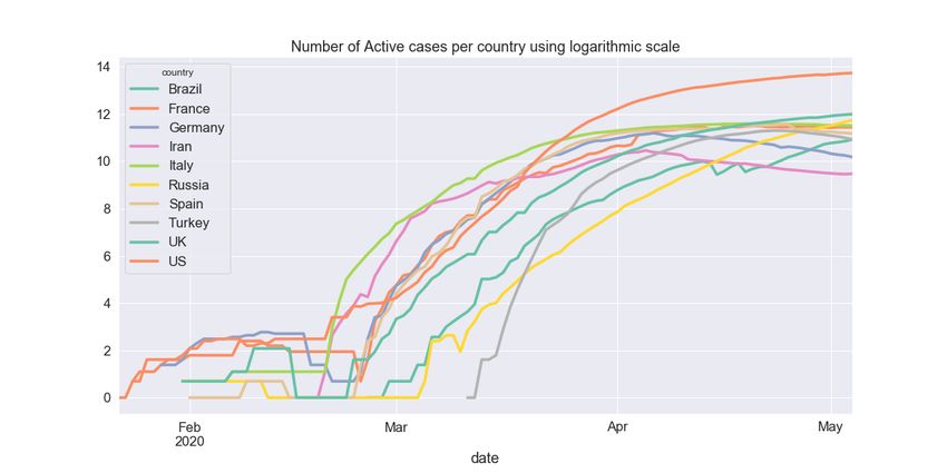
Appl. Sci. 2020, 10, 3880                                                                             2 of 15

spread of the disease and therefore the timing of its peak is to be able to accurately estimate the the
number of active cases at any given point in time.
     In this study, the use of statistical and machine learning-inspired time series methods was
proposed to estimate the percentage of active cases with respect to the total population for the ten
countries with the most active cases. More specifically, six different time series approaches, namely
ARIMA [14], the Holt–Winters additive model (HWAAS) [15], TBAT [16], Facebook’s Prophet [17],
DeepAR [18] (as implemented in [19]) and N-Beats [20], were developed and then compared for
each of the following countries: USA, UK, Italy, Spain, Russia, France, Turkey, Germany, Iran
and Brazil. In terms of evaluation metrics, the root mean square error (RMSE) was employed to
assess the performance of each time series model. The results indicate that, although there is not a
one-size-fits-all approach when it comes to predicting active cases for different countries, ARIMA and
TBAT demonstrate superior performance in seven out of ten countries, while achieving second best
results in another two.

2. Related Work
      In this section, scientific work related to this study is presented. Broadly, this includes: (1) older
studies that employ machine learning and statistical approaches to capture the patterns and trends of a
number of varying events related to infectious diseases; and (2) newer studies that use such approaches
but strictly focus on predicting COVID-19 outbreak related statistics such as active cases and deaths.
      Machine learning and statistical methods, which time series forecasting is a subset of, have
been successfully implemented in the past in the area of infectious diseases. Examples include
modeling leptospirosis and its relationship to rainfall and temperature [21] as well as temporal
correlations between the monthly number of Plasmodium falciparum cases and El Niño Southern
Oscillation (ENSO) [22].
      Similar approaches have also been followed to model diseases that occur in cyclic or repeating
patterns, such as the seasonal influenza, for which a number of studies that use time-series modeling
to predict future outbreaks have been published. In [23], an ARIMA [24] model is developed to predict
the monthly incidence of influenza in China for 2012, while, in [25], a time-series prediction model
(Tempel) is proposed for the mutation prediction of influenza A viruses. More examples include
the works of Lee et al. [26], who built a time-series model using weekly time-series flu-related tweet
counts and applied it to provide real-time assessment of influenza spread, and Zhang et al. [27],
who constructed a SARIMA [24] model using Australian influenza surveillance and local Internet
search query data to predict seasonal influenza epidemics in the northern hemisphere, more specifically
in the USA, UK and China. In [28], time-series modeling is used to investigate the role of climate
factors on the epidemiology of influenza transmission in two warm-climate regions, Hong Kong and
Maricopa County (Arizona U.S), whereas Dominguez et al. [29], using another time-series approach,
aimed to examine the behavior of two indicators of influenza activity in the area of Barcelona in order
to improve the its detection rate.
      Regarding COVID-19 forecasting, there has been a surge in scientific work published during the
last few months. The majority of these studies focus on predicting coronavirus-related metrics such as
active cases and deaths in China, where the disease originally appeared.
      In [30], real-time forecasts regarding the cumulative number of reported cases in China
provinces are produced using three different phenomenological models, previously utilized to
forecast infectious diseases such as SARS, Ebola, pandemic influenza and dengue. In a related
study, Yang et al. [31] integrated population migration data and epidemiological data to train a
Susceptible–Exposed–Infectious–Removed (SEIR) model and combined it with artificial intelligence
models trained on the 2003 SARS data to predict the epidemic curve in China. In [32], the daily and
total number of infections and deaths as well as the corresponding turning points of the pandemic
in China are modeled using a symmetrical function. A modified stacked auto-encoder is developed
in [33] to model the transmission dynamics of the epidemic and forecast the number of confirmed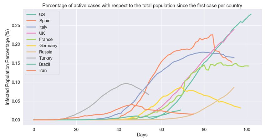
Appl. Sci. 2020, 10, 3880                                                                          3 of 15

COVID-19 cases across China, while Al-qaness et al. [34] proposed a combination of an adaptive
neuro-fuzzy inference system (ANFIS) and a salp-swarm-algorithm-enhanced (SSA) flower pollination
algorithm (FPA) in order to predict the confirmed cases of COVID-19 in the next ten days.
      In [35], a study including China but also two European countries, Italy and France, simple
mean-field models were employed to predict the spread of the pandemic and most notably the height
and timing of its peak in each of these countries.
      The basic reproductive number (R0) was estimated in three different studies: Wu et al. [36]
used Markov Chain Monte Carlo (MCMC) methods; Anastassopoulou et al. [37] proposed a
Susceptible–Infectious–Recovered–Dead (SIDR) model; and Zhang et al. [38], in a study very specific
to the Diamond Princess cruise ship, fit statistical distributions to estimate the R0 in the early stage
of COVID-19 outbreak. It is worth noting that daily infection mortality and recovery rates as well as
the evolution of the outbreak in the following three weeks are also predicted in [37] by calibrating the
parameters of the SIRD model.
      Statistical modeling was at the heart of the approach followed by IHME COVID-19 health service
utilization forecasting team [39], who predicted the strain that would be caused by the pandemic in
United States health system by estimating the numbers of hospital beds, ICU beds and ventilators that
would be needed in the next four months as well as the number of deaths.
      Finally, in another work closely related to this study, Petropoulos and Makridakis [40] adopted
simple time series forecasting approaches, using models from the exponential smoothing family, to
predict the number of confirmed COVID-19 cases on a global scale.

3. Description of Time Series Models
     Time series forecasting is forecasting area that focuses on analyzing past observations of a random
variable to develop a model that best captures the underlying relationship and its patterns. The
model is then used to predict the future values of that random variable. This approach is particularly
useful in two cases: when there is little or no knowledge available on the underlying data-generating
distribution/process or when there is no explanatory model that is able to adequately relate the
prediction variable to other explanatory variables. Over the past several decades, a lot of effort
and research output has been produced towards the development and improvement of time series
forecasting models.
     In this section, six different forecasting methods are presented and briefly analyzed: ARIMA [14],
the Holt–Winters additive model (HWAAS) [15], TBAT [16], Facebook’s Prophet [17], DeepAR
(as implemented in [19]) [18] and N-Beats [20].

3.1. ARIMA: Auto-Regressive Integrated Moving Average
     One of the most well-known and widely used families of time-series models includes the
auto-regressive integrated moving average (ARIMA) models—originally developed for economics
applications [14,41]. Their statistical properties, the implementation of the well-known Box–Jenkins
methodology during model training process [42] and their ability to implement various exponential
smoothing models have all contributed to their popularity and widespread adoption [41,43].
     ARIMA models assume a linear correlation between the time-series values and attempt to
exploit these linear dependencies in observations, in order to extract local patterns, while removing
high-frequency noise from the data [24].
     Such an approach comes with two clear benefits. Firstly, it offers a high level of interpretability,
as, based on the assumptions of the model, the relationship between the independent variables and
the dependent variables are well-understood and therefore easily explained. This enables researchers
to gain a deep understanding not only of the relationship between the current state as a function of
the past states (endogenous variables), but also of any influence inputs outside the state of the series
might have (exogenous variables). The second benefit concerns model selection, which for ARIMA
models can be performed in an automated way to maximize prediction accuracy [44].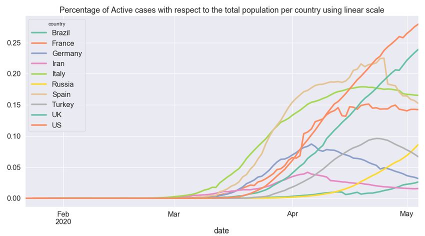
Appl. Sci. 2020, 10, 3880                                                                           4 of 15

     Another benefit of ARIMA models is their ability to accommodate systems governed by dynamics
that change over time by updating the model based on recent events to predict the future state of the
system [44].
     However, since the ARIMA models cannot deal with nonlinear patterns or relationships, their
approximation of complex real-world problems and dynamics is not always satisfactory [45].

3.2. Holt–Winters Additive Model (HWAAS): Exponential Smoothing with Additive Trend and
Additive Seasonality
     The Holt–Winters additive model is an extension of Holt’s exponential smoothing, a time series
forecasting method for univariate data. It is extended so that it adds the seasonality factor to the
trended forecast, being to model data with a systematic trend or seasonal component. It is a simple yet
powerful and widely used forecasting method which, as mentioned, can cope with trend and seasonal
variation and may be used as an alternative to the popular Box–Jenkins ARIMA family of methods.
However, empirical studies have tended to show that the method is not as accurate on average as the
more complicated Box–Jenkins procedure [15].
     Exponential smoothing is the procedure of continuously revising a prediction after taking into
account the more recent observations. In practice, this is achieved by exponentially diminishing the
older observations’ importance for forecasting by decreasing their weights. In other words, when it
comes to predicting a new value, more recent observations matter more than older ones [46].
     The Holt–Winters additive model is best for data with trend and seasonality that do not increase
over time and results in a curved forecast that shows the seasonal changes in the data. Practical issues
in implementing the method include the choice of initial values, their sensitivity to unusual events or
outliers, the choice of smoothing parameters and the normalization of seasonal indices [47,48].

3.3. TBAT
     The identifier TBAT is an acronym for the four fundamental components of the method:
Trigonometric seasonal formulation [49], Box–Cox transformation [50], ARMA errors [24] and trend
component. The method relies on trigonometric functions to model non-integer seasonal frequencies
and Box–Cox transformations to transform non-normal dependent variables into a normal shape and
allow certain types of nonlinearity. As demonstrated through three empirical studies [16], the method
can be applied to a wide range of time-series problems.
     In addition to being computationally effective for maximum likelihood estimators, its
proposed trigonometric formulation allows the decomposition of complex seasonal time series.
This decomposition has been shown to often enable the identification and extraction of seasonal
elements which would not be visible in the time series plot [16].
     Other key advantages of the TBAT modeling framework include a large parameter space with the
possibility of better forecasts [51], handling of the nonlinear features typically seen in real-world time
series data, consideration of any auto-correlation in the residuals and a simple yet efficient estimation
procedure overall [16].

3.4. Prophet: Automatic Forecasting Procedure
     Prophet is a time series forecasting model developed by Facebook and was originally designed to
handle business time series problems. Although there is a wide diversity of methods for predicting
business-related outcomes, many business problems share the same pool of common features such as
seasonal effects [17].
     The method uses an easily decomposable time-series model [52] consisting of three main
components: trend, seasonality and holidays. In its core, it is regression model with interpretable
parameters that often work well with their default values, while also allowing the user to intuitively
choose the components that concern their forecasting problem and effortlessly apply the necessary
adjustments [17].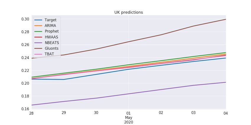
Appl. Sci. 2020, 10, 3880                                                                               5 of 15

      To forecast trend, prophet employs two models: a saturating growth model and a piece-wise
linear model. For growth predictions, a model similar to population growth models in natural
ecosystems [53] is used, where there is nonlinear growth that reaches a saturation point at a carrying
capacity. For forecasting problems where this saturating point is never reached, a piece-wise model of
constant growth-rate provides an efficient and often useful solution. To capture seasonality, prophet
relies on Fourier series to provide a flexible model of periodic effects [54], while, to account for holidays,
a predefined list of past and future holiday events is required. Holiday effects are assumed to be
independent and therefore incorporating them to the model becomes a trivial task [17].

3.5. DeepAR: Probabilistic Forecasting with Auto-Regressive Recurrent Networks
      DeepAR is a forecasting method based on autoregressive recurrent neural networks for
probabilistic forecasting. The method approaches the forecasting problem by incorporating appropriate
likelihoods and combining them with nonlinear data transformation techniques, as learned by a (deep)
neural network [18].
      The method utilizes a long short-term memory based recurrent neural network architecture,
as described in [55], while also building on top of previous work on deep learning for time series
data [56–58] to address the probabilistic forecasting problem. Deeper networks, as described in [59],
allow for more abstract data representations through more complex transformations and therefore are
often preferable to shallow and wide neural networks.
      DeepAR offers three distinct benefits: Firstly, it produces probabilistic predictions in the form of
Monte Carlo samples that can be utilized to calculate consistent quantile estimates for all sub-ranges in
the forecasting scope. Secondly, by not assuming Gaussian noise, the method can support a broad range
of likelihood functions, thus allowing the user to pick the one that best fits the statistical properties
of the data. Lastly, as a deep-learning based method, it is capable of learning seasonal behaviors and
complex dependencies with minimal manual intervention [18].

3.6. N-Beats: Neural Basis Expansion Analysis for Interpretable Time Series Forecasting
     N-Beats is times series forecasting model that employs a deep neural architecture consisting
of forward and backward residual links along with a deep stack of fully-connected layers [20].
Generally, the model operates in the same way as traditional decomposition techniques, such as
the seasonality-trend-level approach [60].
     More specifically, the architecture is comprised of two stacks: the trend stack, followed by the
seasonality stack—each consisting of several blocks connected using residual connections. Combined
with the forecast/backcast principle, this dual residual stacking results in the trend component being
detached from the input window before it is passed into the seasonality stack. Therefore, the partial
forecasts of trend and seasonality are decoupled from one another, becoming available as separate
output, which brings a much-desirable layer of interpretability to the model [20].
     In addition to interpretability and accuracy benefits, as measured on several well-known datasets,
the model is very fast to train and can be applied with few, if any, adjustments to a wide array of target
domains [20].

4. COVID-19 Data: Deaths, Confirmed, Recovered
    As a result of the outbreak, many organizations and individuals have created publicly available
datasets regarding COVID-19 data for analysis and research. One of the most popular attempts is the
White House in collaboration leading research groups, in order to provide a dataset of over 51,000
scholarly articles, including over 40,000 with full text, about COVID-19, SARS-CoV-2 and related
coronaviruses.
    In this study, two publicly available datasets, accessible on kaggle.com, were used for
model development and analysis purposes: the “Novel Corona Virus 2019 Dataset” [61] and the
population-by-country dataset [62]. For access to both datasets see Appendix A.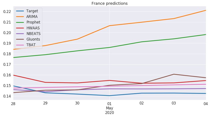
Appl. Sci. 2020, 10, 3880 6 of 15
The former is comprised of time-series information concerning the progression of the virus in each
country, while the latter was used to extract, model and forecast the active virus cases as a percentage
of the total population for each country. This was accomplished by diving each time-series value by
the total population during training, evaluation and testing, allowing for a more clear picture to be
formed as well for more fair comparison to be drawn between the spread rate of the disease among
the different countries.
The “Novel Corona Virus 2019 Dataset” contains daily information regarding:
1. The number of confirmed COVID-19 cases
2. The number of recovered COVID-19 patients
3. The death toll due to COVID-19
The number of active cases in each country for each day was calculated by subtracting both the
recovered patients and the number of deaths from the confirmed cases.
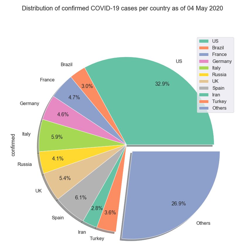
The distribution of total confirmed cases per country as of 4 May 2020 is displayed in Figure 1,
while Figure 2 shows the number of active cases, also as of 4 May 2020, ar using logarithmic scale.
Based on the statistics presented is Figure 1, the 10 countries with the greatest number of total
confirmed cases were kept, accounting, as of 4 May 2020, for more than 70% of all confirmed cases
worldwide. These countries, being the most affected by the virus and probably in later stages of the
pandemic could act as a reference point and a paradigm for newly-infected countries.
Figure 1. Distribution of cumulative confirmed COVID-19 cases per country as of 4 May 2020.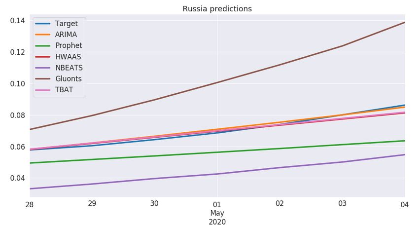
Appl. Sci. 2020, 10, 3880                                                                                     7 of 15

                            Figure 2. Number of active cases per country using logarithmic scale.

     Lastly, the percentage of active cases with respect to the total population per country is shown for
each country in Figures 3 and 4. In the former, the spread of the pandemic is shown for each country
throughout the whole period since January, while, in the latter, the first confirmed case in each country
is used as moment zero. This alignment between the different time series data could help form a better
picture and gain a deeper understanding of the spread of the pandemic in each of these ten countries
as well as better knowledge of the stage of the pandemic in each country.

      Figure 3. Percentage of active cases with respect to the total population per country using linear scale.
Appl. Sci. 2020, 10, 3880 8 of 15
Figure 4. Percentage of active cases with respect to the total population per country. For each country,
moment zero is the first confirmed case in that country.
5. Experiments and Results
In this section, the development and evaluation procedures for all six approaches, namely
ARIMA [14], the Holt–Winters additive model (HWAAS) [15], TBAT [16], Facebook’s Prophet [17],
DeepAR [18] (as implemented in [19]) and N-Beats [20], are described in detail, while also the final
results are presented and discussed. For the source code regarding the implementation see Appendix A.
5.1. Modeling Process
The aim of the study was to compare time series methods in regard to predicting the percentage
of active COVID-19 cases with respect to the total population.
To this end, the ten countries with the greatest number of total confirmed cases were selected to
experiment with and draw comparisons from, as they account for more than 70% of the confirmed
cases globally.
Each time series model was trained, evaluated and tested using time series representing
percentages of active cases with regards to the total population of each of the ten countries.
For each country, 104 instances were created, each representing the percentage of active
coronavirus cases as a fraction of the total population for a single day in the corresponding country.
The number of active cases in each country for each day was calculated by subtracting both the
recovered patients and the number of deaths from the confirmed cases, while the percentage of the
total population that these active correspond to was calculated by dividing each day’s active-cases
value by the population of the respective country.
For training and validation purposes, 97 of these instances were used (72 for training and 25 for
validation), while a window of seven days was kept aside to evaluate the performance of the predictive
models described in Section 3. In terms of the evaluation metric, the root mean squared error (RMSE)
was used to assess the predictive power of each of the approaches.
5.2. Model Performance
Performance results of each model for each country are presented in Table 1, indicating that, in
terms of RMSE, there is no one-size-fits-all approach for predicting the percentage of active cases with
respect to the total population for different countries.Appl. Sci. 2020, 10, 3880 9 of 15
Table 1. Model performance in terms of RMSE for ten countries with the most confirmed COVID-19
cases as of 4 May 2020.
US Spain Italy UK France
ARIMA 0.007421 0.080094 0.005628 0.005484 0.060824
Prophet 0.013877 0.065433 0.019217 0.007634 0.044482
HWAAS 0.172957 0.031497 0.006616 0.004366 0.011007
NBEATS 0.036958 0.050492 0.008645 0.037623 0.004220
Gluonts 0.044805 0.108842 0.043551 0.046134 0.010549
TBAT 0.009873 0.029295 0.005810 0.004310 0.007003
Germany Russia Turkey Brazil Iran
ARIMA 0.006431 0.001536 0.004442 0.004194 0.002628
Prophet 0.037139 0.014681 0.044595 0.009279 0.016281
HWAAS 0.004586 0.002295 0.000887 0.005717 0.001046
NBEATS 0.013192 0.027078 0.018265 0.010870 0.003745
Gluonts 0.057523 0.034479 0.093839 0.002836 0.002277
TBAT 0.003389 0.002193 0.001946 0.005621 0.000425
Moreover, in terms of statistical testing, the Friedman non-parametric multiple groups test [63]
with a significance level of α = 0.02 was applied to produce the corresponding ranking between the
algorithms, as shown in Table 2
Table 2. Friedman statistical test ranking (significance level of α = 0.02).
Rank Algorithm
1.70000 TBAT
2.90000 ARIMA
2.90000 HWAAS
4.10000 NBEATS
4.60000 Prophet
4.80000 Gluonts
Overall, as demonstrated both by RMSE-measured performance (Table 1) and by the statistical
ranking (Table 2), statistical approaches such as ARIMA, TBAT and HWAAS outperform the deep
learning methods such as N-BEATS and DeepAR (GluonTS), which is probably a result of the lack of
high volumes of data that deep-learning algorithms need to thrive.
It is also worth noting that Facebook’s Prophet did not achieve superior performance in any of the
countries, which did not come as a big surprise, given that the method was fundamentally developed
to deal with business problems.
That said, firstly TBAT and secondly ARIMA seem to be the best performing methods overall,
providing, in terms of RMSE, the best predictions in a combined seven countries, while also achieving
second best results in another two. More specifically, ARIMA provided superior performance in terms
of RMSE in the USA, Italy and Russia (Figure 5), while TBAT achieved the best results in Spain, the
UK (Figure 6), Germany and Iran.
Delving deeper into TBAT, in nine out of ten cases, it made it into the top two, with the exception
of Brazil where it achieved third-best performance, behind Gluonts and ARIMA.
Furthermore, in terms of statistical testing, when Holm’s post-hoc statistical analysis [64] was
applied on top of Friedman’s test, it proved that, by using significance level of α = 0.02, TBAT is
significantly better than Prophet, DeepAR (Gluonts) and N-BEATS, as illustrated in Table 3.
Further into statistical time series methods, regarding ARIMA and HWAAS, while the former
performed better overall than the latter, both achieved top-three performance in seven out of ten cases
with the Holt–Winters additive model producing the best results in Turkey.Appl. Sci. 2020, 10, 3880 10 of 15
Lastly, as far as deep learning methods are concerned, although N-BEATS and DeepAR (Gluonts)
offered poor performance overall, they achieved superior results in France (Figure 7) and Brazil,
respectively.
Table 3. TBAT vs All: Holm’s post-hoc statistical analysis was applied on top of Friedman’s test
(significance level of α = 0.02).
Comparison Statistic Adjusted p-Value Result
TBAT vs Gluonts 3.70521 0.00106 H0 is rejected
TBAT vs Prophet 3.46616 0.00211 H0 is rejected
TBAT vs NBEATS 2.86855 0.01237 H0 is rejected
TBAT vs ARIMA 1.43427 0.30299 H0 is accepted
TBAT vs HWAAS 1.43427 0.30299 H0 is accepted
Figure 5. Predictions for Russia.
Figure 6. Predictions for the UK.Appl. Sci. 2020, 10, 3880 11 of 15
Figure 7. Predictions for France.
5.3. Cross-Country Comparison
It is hard to pinpoint the exact reasons certain algorithms perform better than others in one
country but not in others.
Among the factors that should be noted are the following:
1. Country-specific climatic and geographical characteristics
2. Different population-related attributes such as population density among the different countries
3. Discrepancies in testing and measuring procedures and therefore data collection among the
different countries
4. Diversity in terms of quarantine and other social distancing measures implemented in the
different countries as well as the timing, duration and severity of such measures
6. Conclusions
Knowledge of the percentage of COVID-19-infected population in a country and therefore of
when the outbreak will peak has the potential to substantially reduce the impact of the pandemic, as it
would enable governments to modify their social- and health-related policies ahead of time.
In this study, six different statistical and machine learning-inspired time series methods were
developed to estimate the percentage of active cases with respect to the total population, looking seven
days ahead, for the ten countries with the highest number of confirmed cases as of 4 May 2020.
Using the root mean square error (RMSE) to assess the performance of each time series model,
this work compares the different approaches; results indicate that, although a one-size-fits-all approach
does not exist, traditional statistical methods such as such ARIMA and TBAT overall prevail over
deep learning counterparts such as DeepAR and N-BEATS—an outcome which, due to thelack of
large amounts of data, did not come as a surprise. More specifically, the former two approaches
produced the best overall performance, showing superior predictive power in seven out of ten cases
and achieving a close second in two. In terms of statistical analysis, Friedman’s test was applied to
produce the relative ranking of the algorithms, while Holm’s post-hoc statistical analysis proved that,
by using significance level of α = 0.02, TBAT is significantly better than Prophet, DeepAR (Gluonts)
and N-BEATS.Appl. Sci. 2020, 10, 3880 12 of 15
Cross-country performance was hard to explain and interpret; however, important factors
that should be noted include discrepancies among the different countries in terms of climatic and
geographical characteristics; in terms of population-related characteristics such as density; in terms of
COVID-19 measuring and testing procedures; and in terms of timing, duration and severity of any
social distancing measures (if any) that were implemented.
Finally, future modifications to further improve the predictive accuracy of the models include the
creation of ensembles of the presented models that would combine the best of many worlds in order
to reduce the overall error as well as the adoption multivariate time series modeling that take into
account other factors that are either directly or indirectly related to the spread of the pandemic. Such
data could be related to the overall country or population characteristics that change very slowly over
time, such as density or geographical attributes, but could also be time-series data such as temperature
or humidity changes during the period of the pandemic, or data quantifying the timing, severity and
duration of social distance measures, an example being air quality data in the different countries or
regions over time. Another future ambition would be to use some form of transfer learning in order to
bring learnings from one country to another.
Author Contributions: Conceptualization, S.K.; data curation, P.L. and V.P.; formal analysis, P.L. and V.P.;
investigation, V.P. and P.L.; methodology, V.P. and P.L.; project administration, S.K.; software, P.L. and V.P.;
supervision, S.K.; validation, V.P. and P.L.; visualization, P.L. and V.P.; writing—original draft preparation, V.P.
and P.L.; and writing—review and editing, V.P. All authors have read and agreed to the published version of the
manuscript.
Funding: This research received no external funding.
Conflicts of Interest: The authors declare no conflict of interest.
Appendix A
All datasets [61,62] as well as the necessary code used in this study to parse the data; develop,
train, optimize and evaluate the models; and draw the graphs can be found at the following
public GitHub repository: https://github.com/ML-Upatras/COVID-19-A-comparison-of-time-series-
methods-foractive-cases-forecasting.
References
1. World Health Organization. Naming the Coronavirus Disease (COVID-19) and the Virus that Causes it.
World Health Organization. 2020. Available online: https://www.who.int/emergencies/diseases/novel-
coronavirus-2019/technical-guidance/naming-the-coronavirus-disease-(covid-2019)-and-the-virus-that-
causes-it (accessed on 2 May 2020).
2. Coronaviridae Study Group. The species Severe acute respiratory syndrome-related coronavirus: classifying
2019-nCoV and naming it SARS-CoV-2. Nat. Microbiol. 2020, 5, 536. [CrossRef]
3. Lu, H.; Stratton, C.W.; Tang, Y.W. Outbreak of Pneumonia of Unknown Etiology in Wuhan China:
The Mystery and the Miracle. J. Med Virol. 2020, 92, 401–402. [CrossRef]
4. Fernandes, N. Economic Effects of Coronavirus Outbreak (COVID-19) on the World Economy. 2020.
Available online: https://papers.ssrn.com/sol3/papers.cfm?abstract_id=3557504 (accessed on 4 May 2020)
5. J. CSSE. Coronavirus COVID-19 Global Cases by the Center for Systems Science and Engineering (CSSE) at
Johns Hopkins University (JHU). 2020. Available online: https://coronavirus.jhu.edu/map.html (accessed on
4 May 2020)
6. McCloskey, B.; Zumla, A.; Ippolito, G.; Blumberg, L.; Arbon, P.; Cicero, A.; Endericks, T.; Lim, P.L.;
Borodina, M.; M.G.E. Group. Mass gathering events and reducing further global spread of COVID-19:
A political and public health dilemma. Lancet 2020, 395, 1096. [CrossRef]
7. Preiser, W.; Van Zyl, G.; Dramowski, A. COVID-19: Getting ahead of the epidemic curve by early
implementation of social distancing. S. Afr. Med J. 2020, 110, 1. [CrossRef]
8. Klompas, M. Coronavirus Disease 2019 (COVID-19): Protecting hospitals from the invisible. Ann. Intern.
Med. 2020, 172, 619–620. [CrossRef]Appl. Sci. 2020, 10, 3880 13 of 15
9. WHO. Laboratory Testing for Coronavirus Disease 2019 (COVID-19) in Suspected Human Cases: Interim Guidance,
2 March 2020; Technical report; WHO: Geneva, Switzerland, 2020.
10. Roser, M.; Ritchie, H.; Ortiz-Ospina, E. Coronavirus Disease (COVID-19)–Statistics and Research. Our World
Data 2020. Available online: https://ourworldindata.org/coronavirus (accessed on 4 May 2020).
11. Petherick, A. Developing antibody tests for SARS-CoV-2. Lancet 2020, 395, 1101–1102. [CrossRef]
12. Vogel, G. New blood tests for antibodies could show true scale of coronavirus pandemic. Science 2020, 19.
Available online: https://www.sciencemag.org/news/2020/03/new-blood-tests-antibodies-could-show-
true-scale-coronavirus-pandemic (accessed on 4 May 2020). doi:10.1126/science.abb8028 [CrossRef]
13. Pang, J.; Wang, M.X.; Ang, I.Y.H.; Tan, S.H.X.; Lewis, R.F.; Chen, J.I.P.; Gutierrez, R.A.; Gwee, S.X.W.;
Chua, P.E.Y.; Yang, Q.; et al. Potential rapid diagnostics, vaccine and therapeutics for 2019 novel coronavirus
(2019-nCoV): A systematic review. J. Clin. Med. 2020, 9, 623. [CrossRef]
14. Box, G.; Jenkins, G. Time Series Analysis Forecasting and Control/’Holden Day, San Francisco, California, 1970;
John Wiley & Sons: Hoboken, NJ, USA, 2015.
15. Chatfield, C. The Holt–Winters forecasting procedure. J. R. Stat. Soc. Ser. 1978, 27, 264–279. [CrossRef]
16. De Livera, A.M.; Hyndman, R.J.; Snyder, R.D. Forecasting time series with complex seasonal patterns using
exponential smoothing. J. Am. Stat. Assoc. 2011, 106, 1513–1527. [CrossRef]
17. Taylor, S.J.; Letham, B. Forecasting at scale. Am. Stat. 2018, 72, 37–45. [CrossRef]
18. Salinas, D.; Flunkert, V.; Gasthaus, J.; Januschowski, T. DeepAR: Probabilistic forecasting with autoregressive
recurrent networks. Int. J. Forecast. 2019. doi:10.1016/j.ijforecast.2019.07.001 [CrossRef]
19. Alexandrov, A.; Benidis, K.; Bohlke-Schneider, M.; Flunkert, V.; Gasthaus, J.; Januschowski, T.; Maddix, D.C.;
Rangapuram, S.; Salinas, D.; Schulz, J.; et al. Gluonts: Probabilistic time series models in python. arXiv 2019,
arXiv:1906.05264.
20. Oreshkin, B.N.; Carpov, D.; Chapados, N.; Bengio, Y. N-BEATS: Neural basis expansion analysis for
interpretable time series forecasting. arXiv 2019, arXiv:1905.10437.
21. Chadsuthi, S.; Modchang, C.; Lenbury, Y.; Iamsirithaworn, S.; Triampo, W. Modeling seasonal leptospirosis
transmission and its association with rainfall and temperature in Thailand using time–series and ARIMAX
analyses. Asian Pac. J. Trop. Med. 2012, 5, 539–546. [CrossRef]
22. Hanf, M.; Adenis, A.; Nacher, M.; Carme, B. The role of El Ni no southern oscillation (ENSO) on variations
of monthly Plasmodium falciparum malaria cases at the cayenne general hospital, 1996–2009, French Guiana.
Malar. J. 2011, 10, 100. [CrossRef] [PubMed]
23. Song, X.; Xiao, J.; Deng, J.; Kang, Q.; Zhang, Y.; Xu, J. Time series analysis of influenza incidence in Chinese
provinces from 2004 to 2011. Medicine 2016, 95, e3929. [CrossRef]
24. Adhikari, R.; Agrawal, R.K. An introductory study on time series modeling and forecasting. arXiv 2013,
arXiv:1302.6613.
25. Yin, R.; Luusua, E.; Dabrowski, J.; Zhang, Y.; Kwoh, C.K. Tempel: time-series mutation prediction of
influenza A viruses via attention-based recurrent neural networks. Bioinformatics 2020, 36, 2697–2704.
[CrossRef]
26. Lee, K.; Agrawal, A.; Choudhary, A. Forecasting influenza levels using real-time social media streams.
In Proceedings of the 2017 IEEE International Conference on Healthcare Informatics (ICHI), Park City, UT,
USA, 23–26 August 2017; pp. 409–414.
27. Zhang, Y.; Yakob, L.; Bonsall, M.B.; Hu, W. Predicting seasonal influenza epidemics using cross-hemisphere
influenza surveillance data and local Internet query data. Sci. Rep. 2019, 9, 1–7. [CrossRef]
28. Soebiyanto, R.P.; Adimi, F.; Kiang, R.K. Modeling and predicting seasonal influenza transmission in warm
regions using climatological parameters. PLoS ONE 2010, 5, e9450. [CrossRef]
29. Dominguez, A.; Mu noz, P.; Martínez, A.; Orcau, A. Monitoring mortality as an indicator of influenza in
Catalonia, Spain. J. Epidemiol. Community Health 1996, 50, 293–298. [CrossRef] [PubMed]
30. Roosa, K.; Lee, Y.; Luo, R.; Kirpich, A.; Rothenberg, R.; Hyman, J.; Yan, P.; Chowell, G. Real-time forecasts of
the COVID-19 epidemic in China from 5 February to 24 February 2020. Infect. Dis. Model. 2020, 5, 256–263.
[PubMed]
31. Yang, Z.; Zeng, Z.; Wang, K.; Wong, S.S.; Liang, W.; Zanin, M.; Liu, P.; Cao, X.; Gao, Z.; Mai, Z.; et al. Modified
SEIR and AI prediction of the epidemics trend of COVID-19 in China under public health interventions.
J. Thorac. Dis. 2020, 12, 165. [CrossRef] [PubMed]
32. Li, Q.; Feng, W.; Quan, Y.H. Trend and forecasting of the COVID-19 outbreak in China. J. Infect. 2020, 80, 469–496.Appl. Sci. 2020, 10, 3880 14 of 15
33. Hu, Z.; Ge, Q.; Jin, L.; Xiong, M. Artificial intelligence forecasting of covid-19 in china. arXiv 2020,
arXiv:2002.07112.
34. Al-qaness, M.A.; Ewees, A.A.; Fan, H.; Abd El Aziz, M. Optimization method for forecasting confirmed
cases of covid-19 in China. J. Clin. Med. 2020, 9, 674. [CrossRef]
35. Fanelli, D.; Piazza, F. Analysis and forecast of COVID-19 spreading in China, Italy and France. Chaos Solitons Fractals
2020, 134, 109761. [CrossRef]
36. Wu, J.T.; Leung, K.; Leung, G.M. Nowcasting and forecasting the potential domestic and international spread
of the 2019-nCoV outbreak originating in Wuhan, China: a modelling study. Lancet 2020, 395, 689–697.
[CrossRef]
37. Anastassopoulou, C.; Russo, L.; Tsakris, A.; Siettos, C. Data-based analysis, modelling and forecasting of the
COVID-19 outbreak. PLoS ONE 2020, 15, e0230405. [CrossRef]
38. Zhang, S.; Diao, M.; Yu, W.; Pei, L.; Lin, Z.; Chen, D. Estimation of the reproductive number of novel
coronavirus (COVID-19) and the probable outbreak size on the Diamond Princess cruise ship: A data-driven
analysis. Int. J. Infect. Dis. 2020, 93, 201–204. [CrossRef]
39. IHME COVID-19 Health Service Utilization Forecasting Team. Forecasting COVID-19 impact on hospital
bed-days, ICU-days, ventilator-days and deaths by US state in the next 4 months. medRxiv 2020.
doi:10.1101/2020.03.27.20043752. [CrossRef]
40. Petropoulos, F.; Makridakis, S. Forecasting the novel coronavirus COVID-19. PLoS ONE 2020, 15, e0231236.
[CrossRef] [PubMed]
41. Yule, G.U. Why do we sometimes get nonsense-correlations between Time-Series?–a study in sampling and
the nature of time-series. J. R. Stat. Soc. 1926, 89, 1–63. [CrossRef]
42. Wold, H. A Study in Analysis of Stationary Time Series. J. R. Stat. Soc. 1939, 102, 295.
43. McKenzie, E. General exponential smoothing and the equivalent ARMA process. J. Forecast. 1984, 3, 333–344.
[CrossRef]
44. Kane, M.J.; Price, N.; Scotch, M.; Rabinowitz, P. Comparison of ARIMA and Random Forest time series
models for prediction of avian influenza H5N1 outbreaks. BMC Bioinform. 2014, 15, 276. [CrossRef]
45. Zhang, G.P. Time series forecasting using a hybrid ARIMA and neural network model. Neurocomputing
2003, 50, 159–175. [CrossRef]
46. Kalekar, P.S. Time series forecasting using holt-winters exponential smoothing. Kanwal Rekhi Sch. Inf. Technol.
2004, 4329008, 1–13.
47. Chatfield, C.; Yar, M. Holt-Winters forecasting: some practical issues. J. R. Stat. Soc. Ser. 1988, 37, 129–140.
[CrossRef]
48. Gelper, S.; Fried, R.; Croux, C. Robust forecasting with exponential and Holt–Winters smoothing. J. Forecast.
2010, 29, 285–300.
49. Harvey, A.; Koopman, S.J.; Riani, M. The modeling and seasonal adjustment of weekly observations. J. Bus.
Econ. Stat. 1997, 15, 354–368.
50. Box, G.E.; Cox, D.R. An analysis of transformations. J. R. Stat. Soc. Ser. 1964, 26, 211–243. [CrossRef]
51. Hyndman, R.; Koehler, A.B.; Ord, J.K.; Snyder, R.D. Forecasting with Exponential Smoothing: The State Space
Approach; Springer Science & Business Media: Berlin, Germany, 2008.
52. Harvey, A.C.; Peters, S. Estimation procedures for structural time series models. J. Forecast. 1990, 9, 89–108.
[CrossRef]
53. Hutchinson, G.E. An Introduction to Population Ecology; Number 504: 51 HUT; John Wiley & Sons: Hoboken, NJ,
USA, 1978.
54. Harvey, A.C.; Shephard, N. Estimation and Testing of Stochastic Variance Models; Technical report; Suntory and
Toyota International Centres for Economics and Related: London, UK, 1993.
55. Hochreiter, S.; Schmidhuber, J. LSTM can solve hard long time lag problems. In Advances in Neural Information
Processing Systems; MIT Press: Cambridge, MA, USA, 1997; pp. 473–479.
56. Graves, A. Generating sequences with recurrent neural networks. arXiv 2013, arXiv:1308.0850.
57. Oord, A.v.d.; Dieleman, S.; Zen, H.; Simonyan, K.; Vinyals, O.; Graves, A.; Kalchbrenner, N.; Senior, A.;
Kavukcuoglu, K. Wavenet: A generative model for raw audio. arXiv 2016, arXiv:1609.03499.
58. Zaremba, W.; Sutskever, I.; Vinyals, O. Recurrent neural network regularization. arXiv 2014, arXiv:1409.2329.
59. LeCun, Y.; Bengio, Y.; Hinton, G. Deep learning. Nature 2015, 521, 436–444. [CrossRef] [PubMed]Appl. Sci. 2020, 10, 3880 15 of 15
60. Cleveland, R.B.; Cleveland, W.S.; McRae, J.E.; Terpenning, I. STL: A seasonal-trend decomposition. J. Off.
Stat. 1990, 6, 3–73.
61. Novel Corona Virus 2019 Dataset. Available online: https://www.kaggle.com/sudalairajkumar/novel-
corona-virus-2019-dataset (accessed on 4 May 2020).
62. Population by Country Dataset—2020. Available online: https://www.kaggle.com/tanuprabhu/population-
by-country-2020 (accessed on 4 May 2020).
63. Friedman, M. A comparison of alternative tests of significance for the problem of m rankings. Ann. Math. Stat.
1940, 11, 86–92. [CrossRef]
64. Holm, S. A simple sequentially rejective multiple test procedure. Scand. J. Stat. 1979, 6, 65–70.
c 2020 by the authors. Licensee MDPI, Basel, Switzerland. This article is an open access
article distributed under the terms and conditions of the Creative Commons Attribution
(CC BY) license (http://creativecommons.org/licenses/by/4.0/).You can also read