DEEP AUTO-DEFERRING POLICY FOR APPROXIMATING MAXIMUM INDEPENDENT SETS
←
→
Page content transcription
If your browser does not render page correctly, please read the page content below
Under review as a conference paper at ICLR 2020

D EEP AUTO -D EFERRING P OLICY
FOR A PPROXIMATING M AXIMUM I NDEPENDENT S ETS

 Anonymous authors
 Paper under double-blind review

                                             A BSTRACT

         Designing efficient algorithms for combinatorial optimization appears ubiquitously
         in various scientific fields. Recently, deep reinforcement learning (DRL) frame-
         works have gained considerable attention as a new approach: they can automatically
         train a good solver while relying less on sophisticated domain knowledge of the
         target problem. However, the number of stages (until reaching the final solution) re-
         quired by existing DRL solvers is proportional to the size of the input graph, which
         hurts their scalability to large-scale instances. In this paper, we seek to resolve this
         issue by proposing a novel design of DRL’s policy, coined auto-deferring policy
         (AutoDP), automatically stretching or shrinking its decision process. Specifically,
         it decides whether to finalize the value of each vertex at the current stage or defer
         to determine it at later stages. We apply the proposed AutoDP framework to the
         maximum independent set (MIS) problem and its variants under various scenarios.
         Our experimental results demonstrate significant improvement of AutoDP over
         the current state-of-the-art DRL scheme in terms of computational efficiency and
         approximation quality. The reported performance of our generic DRL scheme is
         also comparable with that of the existing solvers for MIS, e.g., AutoDP outperforms
         them for the Barabási-Albert graph with two million vertices.

1    I NTRODUCTION

Combinatorial optimization is an important mathematical field addressing fundamental questions
of computation, where its popular examples include the maximum independent set (MIS, Miller &
Muller 1960), satisfiability (SAT, Schaefer 1978) and traveling salesman problem (TSP, Voigt 1831).
Such problems also arise in various applied fields, e.g., sociology (Harary & Ross, 1957), operations
research (Feo et al., 1994) and bioinformatics (Gardiner et al., 2000). However, most combinatorial
optimization problems are NP-hard to solve, i.e., exact solutions are typically intractable to find in
practical situations. To alleviate this issue, there have been huge efforts in designing fast heuristic
solvers (Biere et al., 2009; Knuth, 1997; Mezard et al., 2009) that generate approximate solutions for
such scenarios.
Recently, the remarkable progress in deep learning has stimulated increased interest in learning such
heuristics based on deep neural networks (DNNs). Such learning-based approaches are attractive
since one could automate the design of approximation algorithms with less reliance on sophisticated
knowledge. As the most straight-forward way, supervised learning schemes can be used for training
DNNs to imitate the solutions obtained from existing solvers (Vinyals et al., 2015; Li et al., 2018;
Selsam et al., 2019). However, such a direction can be criticized, for its quality and applicability
are bounded by those of existing solvers. An ideal direction is to discover new solutions in a fully
unsupervised manner, potentially outperforming those based on domain-specific knowledge.
To this end, deep reinforcement learning (DRL) schemes have been studied in the literature (Bello
et al., 2016; Khalil et al., 2017; Deudon et al., 2018; Kool et al., 2019) as a Markov decision process
(MDP) can be naturally designed with rewards derived from the optimization objective of the target
problem. Then, the corresponding agent can be trained based on existing training schemes of DRL,
e.g., Bello et al. (2016) trained the so-called pointer network for the TSP based on actor-critic training.
Such DRL-based methods are especially attractive since they can even solve unexplored problems
where domain knowledge is scarce and no efficient heuristic is known. However, the existing methods

                                                    1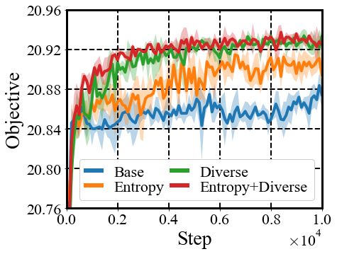
Under review as a conference paper at ICLR 2020

                   Figure 1: Illustration of the proposed Markov decision process.

struggle to compete with the existing highly optimized solvers. In particular, the gap grows larger
when the problem requires solutions with higher dimensions or more complex structures.
Our motivation stems from the observation that existing DRL-based solvers lack efficient policies for
generating solutions to combinatorial problems. Specifically, they are mostly based on emulating
greedy iterative heuristics (Bello et al., 2016; Khalil et al., 2017) and become too slow for training on
large graphs. Their choice seems inevitable since an algorithm that generates a solution based on a
single feed-forward pass of DNN is potentially hard to train due to large variance in reward signals
coming from high dimensional solutions.
Contribution. In this paper, we propose a new scalable DRL framework, coined auto-deferring
policy (AutoDP), designed towards solving combinatorial problems on large graphs. We particularly
focus on applying AutoDP to the MIS problem (and its variants) which attempts to find a maximum
set of vertices in the graph where no pair of vertices are adjacent to each other. Our choice of the
MIS problem is motivated by its hardness and applicability. First, the MIS problem is impossible to
approximate in polynomial time by a constant factor (unless P=NP) (Hastad, 1996), in contrast to
(Euclidean or metric) TSP which can be approximated by a factor of 1.5 (Christofides, 1976). Next,
it has wide applications including classification theory (Feo et al., 1994), computer vision (Sander
et al., 2008) and communication algorithms (Jiang & Walrand, 2010).
The main novelty of AutoDP is automatically stretching the determination of the solution throughout
multiple steps. In particular, the agent iteratively acts on every undetermined vertex for either (a)
determining the membership of the vertex in the solution or (b) deferring the determination to be
made in later steps (see Figure 1 for illustration). Inspired by the celebrated survey propagation
(Braunstein et al., 2005) for solving the SAT problem, AutoDP could be interpreted as prioritizing
the “easier” decisions to be made first, which in turn simplifies the harder ones by eliminating the
source of uncertainties. Compared to the greedy strategy (Khalil et al., 2017) which determines the
membership of a single vertex at each step, our framework brings significant speedup by allowing
determinations on as many vertices as possible to happen at once.
Based on such speedup, AutoDP can solve the optimization problem by generating a large number of
candidate solutions in a limited time budget, then reporting the best solution among them. In such a
scenario, it is beneficial for the algorithm to generate diverse candidates. To this end, we additionally
give a novel diversification bonus to our agent during training, which explicitly encourages the agent
to generate a large variety of solutions. Specifically, we create a “coupling” of MDPs to generate
two solutions for the given MIS problem and reward the agents for a large deviation between the
solutions. The resulting reward efficiently stimulates the agent to explore high-dimensional input
spaces and to improve the performance at the evaluation.
We empirically validate the AutoDP method on various types of graphs including the Erdös-Rényi
(Erdős & Rényi, 1960) model, the Barabási-Albert (Albert & Barabási, 2002) model, the SATLIB
(Hoos & Stützle, 2000) benchmark and real-world graphs (Hamilton et al., 2017; Yanardag &
Vishwanathan, 2015; Leskovec & Sosič, 2016). Our algorithm shows consistent superiority over
the existing state-of-the-art DRL method (Khalil et al., 2017) both in terms of speed and quality of
the solution, and can compete with the existing MIS solver (ReduMIS, Lamm et al. 2017) under
a similar time budget. For example, AutoDP even outperforms ReduMIS in the Barabási-Albert
graph with two million vertices using a smaller amount of time. Furthermore, we also show that our
fully learning-based scheme generalizes well even to graph types unseen during training and works
well even for other variants of the MIS problem: the maximum weighted independent set (MWIS)
problem and the prize collecting maximum independent set (PCMIS) problem (see Appendix B).
This sheds light on its potential of being a generic solver that works for arbitrary large-scale graphs.

                                                   2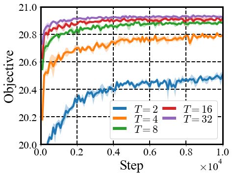
Under review as a conference paper at ICLR 2020

2     R ELATED WORKS
The maximum independent set (MIS) problem is a prototypical NP-hard task where its optimal solu-
tion cannot be approximated by a constant factor in polynomial time (unless P = NP) (Hastad, 1996),
although it admits a nearly linear factor approximation algorithm (Boppana & Halldórsson, 1992). It
is also known to be a W [1]-hard problem in terms of fixed-parameter tractability (Downey & Fellows,
2012). Since the problem is NP-hard, existing methods (Tomita et al., 2010; San Segundo et al., 2011)
for exactly solving the MIS problem often suffers from a prohibitive amount of computation in large
graphs. To resolve this issue, a wide range of solvers have been developed for approximately solving
the MIS problem (Grosso et al., 2008; Andrade et al., 2012; Dahlum et al., 2016; Lamm et al., 2017;
Chang et al., 2017; Hespe et al., 2019). Notably, Lamm et al. (2017) developed a combination of an
evolutionary algorithm with graph kernelization techniques for the MIS problem. Later, Chang et al.
(2017) and Hespe et al. (2019) further improved the graph kernelization technique by introducing
new reduction rules and parallelization based on graph partitioning, respectively.
In the context of solving combinatorial optimization using neural networks, Hopfield & Tank (1985)
first applied the Hopfield-network for solving the traveling salesman problem (TSP). Since then,
several works also tried to utilize neural networks in different forms, e.g., see Smith (1999) for a
review of such papers. Such works were mostly used for solving combinatorial optimization through
online learning, i.e., training was performed for each problem instance separately. More recently,
(Vinyals et al., 2015) and (Bello et al., 2016) proposed to solve TSP using an attention-based neural
network trained in an offline way. They showed promising results that stimulated many other works
to use neural networks for solving combinatorial problems (Khalil et al., 2017; Selsam et al., 2019;
Deudon et al., 2018; Amizadeh et al., 2018; Li et al., 2018; Kool et al., 2019). Importantly, Khalil
et al. (2017) proposed a reinforcement learning framework for solving the minimum vertex cover
problem, which is equivalent to solving the MIS problem. They query the agent for each vertex to
add as a new member of the vertex cover at each step of the Markov decision process. However,
such a procedure often leads to a prohibitive amount of computation on graphs with large vertex
covers. Next, Li et al. (2018) aim for developing a supervised learning framework for solving the
MIS problem. At an angle, their framework is similar to ours since they use hand-designed rules to
defer the solution generation procedure at each step. However, it is hard to fairly compare with ours
since the supervised learning scheme is highly sensitive to the quality of solutions obtained from
existing solvers and is often too expensive to apply, e.g., for the MIS-variants.

3     D EEP AUTO - DEFERRING POLICY
In this paper, we focus on solving the maximum independent set (MIS) problem. Given a graph
G = (V, E) with vertices V and edges E, an independent set is a subset of vertices I ⊆ V where
no two vertices in the subset are adjacent to each other. A solution to the MIS problem can be
represented
P             as a binary vector x = [xi : i ∈ V] ∈ {0, 1}V with maximum possible cardinality
   i∈V ix , where  each element xi indicates the membership of vertex i in the independent set I, i.e.,
xi = 1 if and only if i ∈ I. Initially, the algorithm has no assumption about its output, i.e., both
xi = 0 and xi = 1 are possible for all i ∈ V. At each iteration, the agent acts on each undetermined
vertex i by either (a) determining its membership to be a certain value, i.e., set xi = 0 or xi = 1, or
(b) deferring the determination to be made later iterations. The iterations are repeated until all the
membership of vertices in the independent set is determined. Such a strategy could be interpreted
as progressively narrowing down the set of candidate solutions at each iteration (see Figure 1 for
illustration). Intuitively, the act of deferring could be seen as prioritizing to choose the values of
the “easier” vertices first. After the decisions are made, decisions on “hard” vertices become easier
since the decisions on its surrounding easy vertices are better known. We additionally provide an
illustration of the whole algorithm in Appendix A.

3.1   D EFERRED M ARKOV DECISION PROCESS

To train the agent via reinforcement learning, we formulate the proposed algorithm as a Markov
decision process (MDP).
State. Each state of the MDP is represented as a vertex-state vector s = [si : i ∈ V] ∈ {0, 1, ∗}V ,
where the vertex i ∈ V is determined to be excluded or included in the independent set whenever

                                                  3
Under review as a conference paper at ICLR 2020
Figure 2: Illustration of the transition function with Figure 3: Illustration of coupled MDP with
the update and the clean-up phases. the corresponding solution diversity reward.
si = 0 or si = 1, respectively. Otherwise, si = ∗ indicates the determination has been deferred and
expected to be made in later iterations. The MDP is initialized with the deferred vertex-states, i.e.,
si = ∗ for all i ∈ V, and terminated when there is no deferred vertex-state left.
Action. Actions correspond to new assignments for the next state of vertices. Since vertex-states
of included and excluded vertices are immutable, the assignments are defined only on the deferred
vertices. It is represented as a vector a∗ = [ai : i ∈ V∗ ] ∈ {0, 1, ∗}V∗ where V∗ denotes a set of
current deferred vertices, i.e., V∗ = {i : i ∈ V, xi = ∗}.
Transition. Given two consecutive states s, s0 and the corresponding assignment a∗ , the transition
Pa∗ (s, s0 ) consists of two deterministic phases: the update phase and the clean-up phase. In the
update phase, the assignment a∗ generated by the policy is updated for the corresponding vertices
V∗ to result in an intermediate vertex-state sb, i.e., sbi = ai if i ∈ V∗ and sbi = si otherwise. In the
cleanup phase, the intermediate vertex-state vector sb is modified to yield a valid vertex-state vector
s0 , where included vertices are only adjacent to the excluded vertices. To this end, whenever there
exists a pair of included vertices adjacent to each other, they are both mapped back to the deferred
vertex-state. Next, any deferred vertex neighboring with an included vertex is excluded. If the state
reaches the pre-defined time limit, all deferred vertices are automatically excluded. See Figure 2 for a
more detailed illustration of the transition.
0
P reward0 R(s, s ) is defined
Reward. Finally, as the increase in cardinality of included vertices, i.e.,
R(s, s ) = i∈V∗ \V∗0 si , where V∗ and V∗0 are the set of vertices with deferred vertex-state with
0
respect to s and s0 , respectively. By doing so, the overall return of the MDP corresponds to the
cardinality of the independent set returned by our algorithm.
3.2 T RAINING WITH DIVERSIFICATION REWARD
Next, we introduce an additional reward term for encouraging diversification of solutions generated
by the agent. Such regularization is motivated by our evaluation method which samples multiple
candidate solutions to report the best one as the final output. For such scenarios, it would be beneficial
to generate diverse solutions of high maximum score, rather than ones of similar scores. One might
argue that the existing entropy regularization (Williams & Peng, 1991) for encouraging exploration
over MDP could be used for this purpose. However, the entropy regularization attempts to generate
diverse trajectories of the same MDP which does not necessarily lead to diverse solutions at last,
since there exist many trajectories resulting in the same solution (see Section 3.1). We instead
directly maximize the diversity among solutions by a new reward term. To this end, we “couple” two
copies of MDPs defined in Section 3.1 into a new MDP by sharing the same graph G with a pair of
distinct vertex-state vectors (s, s̄). Although the coupled MDPs are defined on the same graph, the
corresponding agents work independently to result in a pair of solutions (x, x̄). Then, we directly
reward the deviation between the coupled solutions in terms of `1 -norm, i.e., kx − x̄k1 . Similar to
the original objective of MIS, it is decomposed into rewards in each iteration of the MDP defined as
follows:
X
Rdiv (s, s0 , s̄, s̄0 ) = |s0i − s̄0i |, where V
b = (V∗ \ V∗0 ) ∪ (V̄∗ \ V̄∗0 ),
i∈V
b
where (s0 , s̄0 ) denotes the next pair of vertex-states in the coupled MDP. One can observe that Vb
denotes the most recently updated vertices in each MDP. In practice, such reward Rdiv can be used
along with the maximum entropy regularization for training the agent to achieve the best performance.
See Figure 3 for an example of coupled MDP with the proposed reward.
4Under review as a conference paper at ICLR 2020
Our algorithm is based on actor-critic training with policy network πθ (a|s) and value network
Vφ (s) parameterized by the graph convolutional network (GCN, Kipf & Welling 2017). Each GCN
(n) (n)
consists of multiple layers hn with n = 1, · · · , N where the n-th layer with weights W1 and W2
performs the following transformation on input H:
(n) 1 1 (n)
h(n) (H) = ReLU HW1 + D− 2 AD− 2 HW2 .
Here A, D correspond to adjacency and degree matrix of the graph G, respectively. At the final
layer, the policy and value networks apply softmax function and graph readout function with sum
pooling (Xu et al., 2019) instead of ReLU to generate actions and value estimates, respectively. We
only consider the subgraph that is induced on the deferred vertices V∗ as the input of the networks
since the determined part of the graph no longer affects the future rewards of the MDP. Features
corresponding to the vertices are given as their node degrees and the current iteration-index of MDP.
To train the agent, proximal policy optimization (Schulman et al., 2017) is used. Specifically, networks
are trained for maximizing the following objective:
Y (t)
(t)
Y
(t) (t)
L := Et min A(s ) b ri (θ), A(s )
b clip(ri (θ), 1 − ε, 1 + ε) ,
i∈V i∈V
(t) T
(t) πθ (ai |s(t) ) X 0 (t0 )
ri (θ) = (t)
, A(s)
b = R(t ) + Rdiv − Vφ (s),
πθold (ai |s(t) ) t0 =t
where s(t) denotes the t-th vertex-state vector and other elements of the MDP are defined similarly.
In addition, clip(·) is the clipping function for updating the agent more conservatively and θold is
the parameter of the policy network from the previous iteration of updates.
4 E XPERIMENTS
In this section, we report experimental results on the proposed auto-deferring policy (AutoDP)
described in Section 3 for solving the maximum independent set (MIS) problem. We also pro-
vide evaluation of our AutoDP framework on variants of the MIS problem in Appendix B, which
demonstrates that our framework is applicable to problems different from the original MIS problem.
Experiments were conducted on a large range of graphs varying from small synthetic graphs to
large-scale real-world graphs. We evaluated our AutoDP scheme by sampling multiple solutions
and then reporting the performance of the best solution. The resulting schemes are coined AutoDP-
10, AutoDP-100, and AutoDP-1000 corresponding to the number of samples chosen from 10, 100
and 1000, respectively. We compared our framework with the deep reinforcement learning (DRL)
algorithm by Khalil et al. (2017), coined S2V-DQN, for solving the MIS problem. Note that other
DRL schemes in the literature, e.g., pointer network (Bello et al., 2016), and attention layer (Kool
et al., 2019) are not comparable since they are specialized to TSP-like problems. We additionally
consider three conventional MIS solvers as baselines. First, we consider the theoretically guaranteed
algorithm of Boppana & Halldórsson (1992) based on iterative exclusion of subgraphs, coined ES,
having an approximation ratio O(|V|/(log |V|)2 ) for the MIS problem. Next, we consider the integer
programming solver IBM ILOG CPLEX Optimization Studio V12.9.0 (ILO, 2014), coined CPLEX.1
We also consider the MIS heuristic proposed by Lamm et al. (2017), coined ReduMIS. Note that
we use the implementation of ReduMIS equipped with graph kernelization proposed by Hespe et al.
(2019). We additionally provide evaluation of the AudoDP framework compared to the supervised
learning framework of Li et al. (2018) in Appendix C. Further details of the implementation and
datasets are provided in Appendix E and F, respectively.
4.1 P ERFORMANCE EVALUATION
We now demonstrate the performance of our algorithm along with other baselines on various datasets.
First, we consider experiments on randomly generated synthetic graphs from the Erdös-Rényi (ER,
Erdős & Rényi 1960) and Barabási-Albert (BA, Albert & Barabási 2002) models. Following Khalil
1
Note that CPLEX is able to provide proof of optimality in addition to the solution for the MIS problem.
2
The authors of S2V-DQN only reported experiments with respect to graphs of size up to five hundred.
5Under review as a conference paper at ICLR 2020
Table 1: Performance evaluation on ER and BA datasets. The bold numbers indicate the best
performance within the same category of algorithms. The relative differences shown in brackets are
measured with respect to S2V-DQN.
Traditional DRL-based
Type |V| Value ES CPLEX ReduMIS S2V-DQN AutoDP-10 AutoDP-100 AutoDP-1000
Obj. 7.800 8.844 8.844 8.840 8.844 (+0.1%) 8.844 (+0.1%) 8.844 (+0.1%)
(15, 20)
Time 0.005 0.003 0.024 0.004 0.002 (−60.7%) 0.005 (+15.6%) 0.056 (+1185.5%)
Obj. 13.83 16.57 16.57 16.42 16.55 (+0.7%) 16.57 (+0.9%) 16.57 (+0.9%)
(40, 50)
Time 0.033 0.062 12.374 0.015 0.004 (−73.1%) 0.016 (+9.6%) 0.164 (+1002.0%)
Obj. 17.01 21.11 21.11 20.61 21.04 (+2.1%) 21.10 (+2.4%) 21.11 (+2.4%)
ER (50, 100)
Time 0.117 0.137 24.387 0.030 0.007 (−77.8%) 0.028 (−4.3%) 0.283 (+852.6%)
Obj. 21.59 27.87 27.95 26.27 27.67 (+5.3%) 27.87 (+6.1%) 27.93 (+6.4%)
(100, 200)
Time 0.608 10.748 30.109 0.078 0.029 (−63.5%) 0.085 (+8.5%) 0.666 (+748.7%)
Obj. 29.28 35.76 39.83 35.05 38.29 (+9.2%) 39.11 (+11.6%) 39.54 (+12.8%)
(400, 500)
Time 10.823 30.085 30.432 0.633 0.158 (−75.1%) 0.407 (−35.7%) 2.768 (+336.8%)
Obj. 6.06 7.019 7.019 7.011 7.019 (+0.1%) 7.019 (+0.1%) 7.019 (+0.1%)
(15, 20)
Time 0.003 0.004 0.041 0.005 0.002 (−60.2%) 0.006 (+19.4) 0.064 (+1103.4)
Obj. 14.81 18.91 18.91 18.87 18.91 (+0.2%) 18.91 (+0.2%) 18.91 (+0.2%)
(40, 50)
Time 0.031 0.020 0.396 0.013 0.003 (−79.2%) 0.011 (−18.4%) 0.118 (+778.1%)
Obj. 24.77 32.07 32.07 31.96 32.07 (+0.3%) 32.07 (+0.3%) 32.07 (+0.3%)
BA (50, 100)
Time 0.130 0.038 0.739 0.022 0.003 (−84.7%) 0.018 (−19.0%) 0.199 (+794.3%)
Obj. 49.87 66.07 66.07 65.52 66.05 (+0.8%) 66.07 (+0.8%) 66.07 (+0.8%)
(100, 200)
Time 0.938 0.088 2.417 0.047 0.007 (−85.2%) 0.038 (−19.6%) 0.380 (+703.6%)
Obj. 148.51 204.14 204.14 202.91 204.04 (+0.6%) 204.10 (+0.6%) 204.12 (+0.6)%
(400, 500)
Time 23.277 0.322 15.080 0.177 0.024 (−86.4%) 0.131 (−25.8%) 1.111 (+527.5%)
Table 2: Performance evaluation on SATLIB, PPI, REDDIT, and as-Caida datasets. The bold numbers
indicate the best performance within the same category of algorithms. The relative differences shown
in brackets are measured with respect to S2V-DQN, except for the case of as-Caida dataset where
S2V-DQN underperforms significantly.2
Traditional DRL-based
Type |V| Value CPLEX ReduMIS S2V-DQN AutoDP-10 AutoDP-100 AutoDP-1000
Obj. 426.8 426.9 413.8 423.8 (+2.4%) 424.8 (+2.7%) 425.4 (+2.8%)
SATLIB (1209, 1347)
Time 9.490 30.110 2.260 0.311 (−86.2%) 1.830 (−19.0%) 16.409 (+626.1%)
Obj. 1147.5 1147.5 893.0 1144.5 (+28.2%) 1146.5 (+28.4%) 1147.0 (+28.4%)
PPI (591, 3480)
Time 24.685 30.23 6.285 0.786 (−87.5%) 1.770 (−71.8%) 11.469 (+82.3%)
REDDIT Obj. 370.6 370.6 370.1 370.6 (+0.1%) 370.6 (+0.1%) 370.6 (+0.1%)
(MULTI-5K) (22, 3648)
Time 0.008 0.159 0.076 0.071 (−6.6%) 0.551 (+625.0%) 5.500 (+7136.8%)
REDDIT Obj. 303.5 303.5 302.8 257.4 (−15.0%) 292.6 (−3.4%) 303.5 (+0.2%)
(MULTI-12K) (2, 3782)
Time 0.007 0.188 1.883 0.003 (−99.8%) 0.025 (−98.7%) 0.451 (−76.1%)
REDDIT Obj. 329.3 329.3 328.6 329.3 (+0.2%) 329.3 (+0.2%) 329.3 (+0.2%)
(BINARY) (6, 3782)
Time 0.007 0.306 0.055 0.020 (−63.6%) 0.173 (+214.6%) 2.627 (+4676.4%)
Obj. 20 049.2 20 049.2 324.0 20 049.2 20 049.2 20 049.2
as-Caida (8020, 26 475)
Time 0.477 1.719 601.351 0.812 6.106 62.286
et al. (2017), the edge ratio of ER graphs and average degree of BA graphs are set to 0.15 and 8,
respectively. Datasets are specified by their type of model and an interval for choosing the number
of vertices uniformly at random, e.g., ER-(50, 100) denotes the set of ER graphs generated with the
number of vertices larger than 50 and smaller than 100. Next, we consider experiments on more
challenging datasets with larger sizes, namely the SATLIB, PPI, REDDIT, and as-Caida datasets
constructed from SATLIB benchmark (Hoos & Stützle, 2000), protein-protein interactions (Hamilton
et al., 2017), social networks (Yanardag & Vishwanathan, 2015) and road networks (Leskovec &
Sosič, 2016), respectively. See the appendix for more details on the datasets. The time limit of the
CPLEX and ReduMIS are set to 30 seconds on ER and BA datasets and 1800 seconds on the rest
of the datasets to provide comparable baselines.3 The corresponding results are reported in Table 1
and 2. Note that the ES method was excluded from comparison in large graphs since it required a
prohibitive amount of computation.
In Table 1 and 2, one can observe that our AutoDP algorithms significantly outperform the deep
reinforcement learning baseline, i.e., S2V-DQN, across all types of graphs and datasets. For example,
AutoDP-10 is always able to find a better solution than S2V-DQN much faster. The gap grows larger
in more challenging datasets, e.g., see Table 2. It is also impressive to observe that our algorithm
can find the best solution in seven out of ten datasets in Table 1 and four out of five datasets in Table
3
The solvers occasionally violate the time limit due to their pre-solving process.
6Under review as a conference paper at ICLR 2020
(a) ER-(400, 500) dataset (b) SATLIB dataset
Figure 4: Evaluation of trade-off between time and objective (upper-left side is of better trade-off).
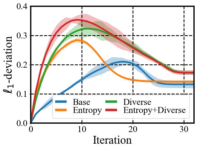
(a) Performance with varying T (b) Contribution of each regularizers (c) Deviation in intermediate stages
Figure 5: Illustration of ablation studies done on ER-(50, 100) dataset. The solid line and shaded
regions represent the mean and standard deviation across 3 runs respectively Note that the standard
deviation in (c) was enlarged ten times for better visibility.
2. Furthermore, we observe that our algorithm achieves better objective than the CPLEX solver on
ER-(100, 200) and ER-(400, 500) datasets, while consuming a smaller amount of time. The highly
optimized ReduMIS solver tends to acquire the best solutions consistently. However, it is often worse
than ours given a limited time budget, as described in what follows.
We investigate the trade-off between objective and time for algorithms in Figure 4. To this end, we
evaluate algorithms on ER-(400, 500) and SATLIB datasets with varying numbers of samples for
AutoDP and time limits for ReduMIS and CPLEX. It is remarkable to observe that AutoDP achieves a
better objective than the CPLEX solver on both datasets under reasonably limited time. Furthermore,
for time limits smaller than 10 seconds, AutoDP outperforms ReduMIS on ER-(400, 500) dataset.
4.2 A BLATION STUDY
We ablate each component of our algorithm to validate its effectiveness. We first show that “stretching”
the determination with deferred MDP indeed helps for solving the MIS problem. Specifically, we
experiment with varying the maximum number of iterations T in MDP by T ∈ {2, 4, 8, 16, 32}
on ER-(50, 100) dataset. Figure 5a reports the corresponding training curves. We observe that the
performance of AutoDP improves whenever an agent is given more time to generate the final solution,
which verifies that the deferring of decisions plays a crucial role in solving the MIS problem.
Next, we inspect the contribution of the solution diversity reward used in our algorithm. To this
end, we trained agents with four options: (a) without any exploration bonus, coined Base, (b) with
the conventional entropy bonus (Williams & Peng, 1991), coined Entropy, (c) with the proposed
diversification bonus, coined Diverse, and (d) with both of the bonuses, coined Entropy+Diverse.
The corresponding training curves for validation scores are reported in Figure 5b. We observe that the
agent trained with the proposed diversification bonus outperforms other agents in terms of validation
score, confirming the effectiveness of our proposed reward. One can also observe that both methods
can be combined to yield better performance, i.e., Entropy+Diverse.
Finally, we further verify our claim that the maximum entropy regularization fails to capture the
diversity of solutions effectively, while the proposed solution diversity reward term does. To this
end, we compare the fore-mentioned agents with respect to the `1 -deviations between the coupled
intermediate vertex-states s and s̄, defined as |{i : i ∈ V, si 6= s̄i }|. The corresponding results are
shown in Figure 5c. One can observe that the entropy regularization leads to large deviations during
the intermediate stages, but converges to solutions with smaller deviations. On the contrary, agents
trained on diversification rewards succeed in enlarging the deviation between the final solutions.
7Under review as a conference paper at ICLR 2020
Table 3: Performance evaluation for large-scale graphs. Out of budget (OB) is marked for runs
violating the time and the memory budget of 10 000 seconds and 32 GB RAM, respectively. The
bold numbers indicate the best performance within the same category of algorithms. The relative
differences shown in brackets are measured with respect to S2V-DQN.
Traditional DRL-based
Type |V| Value CPLEX ReduMIS S2V-DQN AutoDP-10 AutoDP-100 AutoDP-1000
Obj. 434 896 457 349 457 753 457 772
1 000 000 OB OB
Time 5967.82 1802.35 324.02 5112.25
BA
Obj. 909 988 915 553 915 573
2 000 000 OB OB OB
Time 4276.43 772.18 7662.87
Citation Obj. 1451 1451 1393 1451 (+4.2%) 1451 (+4.2%) 1451 (+4.2%)
(Cora) 2708
Time 0.08 0.04 2.57 1.63 (−36.5%) 2.71 (+5.3%) 13.82 (+437.7%)
Citation Obj. 1867 1867 1840 1867 (+1.5%) 1867 (+1.5%) 1867 (+1.5%)
(Citeseer) 3327
Time 0.08 0.03 3.07 1.80 (−41.4%) 2.74 (−10.9%) 19.00 (+518.4%)
Amazon Obj. 2733 2733 725 2705 (+273.1%) 2708 (+273.5%) 2712 (+274.1%)
(Photo) 7487
Time 38.80 39.02 66.53 2.00 (−97.0%) 4.91 (−92.6%) 32.96 (−50.5%)
Amazon Obj. 4829 4829 1281 4773 (+272.6%) 4782 (+273.3%) 4783 (+273.4%)
(Computers) 13 381
Time 188.61 61.78 235.80 3.02 (−98.7%) 8.63 (−96.3%) 79.19 (−66.4%)
Coauthor Obj. 7506 7506 6635 7479 (+12.7%) 7479 (+12.7%) 7483 (+12.8%)
(CS) 18 333
Time 1.50 0.09 197.39 3.03 (−98.5%) 13.23 (−93.3%) 122.44 (−38.0%)
Coauthor Obj. 11 351 11 353 2156 11 176 (+418.4%) 11 186 (+418.8%) 11 190 (+419.0%)
(Physics) 34 493
Time 1802.80 81.34 1564.13 8.63 (−99.5%) 38.71 (−97.5%) 385.93 (−75.3%)
SNAP Obj. 163 385 163 391 160 784 160 837 160 872
(web-Stanford) 281 903 OB
Time 996.25 44.85 13.35 137.98 1357.11
SNAP Obj. 251 846 251 850 250 365 250 384 250 409
(web-NotreDame) 325 729 OB
Time 64.97 1802.34 11.81 119.48 1046.48
SNAP Obj. 125 194 408 483 403 166 403 189 403 231
(web-BerkStan) 685 230 OB
Time 1875.96 100.17 88.67 975.35 9940.93
SNAP Obj. 788 907 784 843 784 891
(soc-Pokec) 1 632 803 OB OB OB
Time 1805.95 770.55 7512.06
SNAP Obj. 986 180 958 980 959 051
(wiki-topcats) 1 791 489 OB OB OB
Time 1060.09 850.80 9121.85
4.3 G ENERALIZATION TO UNSEEN GRAPHS
Now we examine the potential of our method as a generic solver, i.e., whether the algorithm’s
performance generalizes well to graphs unseen during training. To this end, we train AutoDP and
S2V-DQN models on BA-(400, 500) dataset and evaluate them on the following real-world graph
datasets: Coauthor, Amazon (Shchur et al., 2018) and Stanford Network Analysis Platform (SNAP,
Leskovec & Sosič 2016). We additionally evaluate on BA graphs with millions of vertices. We also
evaluate the generalization of the algorithm across synthetic graphs with different types and sizes in
Appendix D. Similar to the experiments in Table 2, we set the time limit on CPLEX and ReduMIS by
1800 seconds. The ES method is again excluded as being computationally prohibitive to compare.
As reported in Table 3, AutoDP successfully generates solutions for large scale instances which
scale up to two million (2M), even though it was trained on graphs of size smaller than five hundred
vertices. Most notably, AutoDP-10 outperforms the ReduMIS (state-of-the-art solver) in BA graph
with 2M vertices, but six times faster. It also outperforms the CPLEX in the graphs with more than
0.5M vertices, indicating better scalability of our algorithm. Note that CPLEX also fails to generate
solutions on graphs with more than 1M vertices. Such a result strongly supports the potential of
AutoDP being a generic solver that could be used in place of conventional solvers. On the contrary,
we found that S2V-DQN does not generalize well to large graphs: it performs worse and takes much
more time to generate solutions as it requires the number of decisions proportional to the graph size.
5 C ONCLUSION
In this paper, we propose a new reinforcement learning framework for the maximum independent set
problem that is scalable to large graphs. Our main contribution is the auto-deferring policy, which
allows the agent to defer the decisions on vertices for efficient expression of complex structures in
the solutions. Through extensive experiments, our algorithm shows performance that is both superior
to the existing reinforcement learning baseline and competitive with the conventional solvers.
8Under review as a conference paper at ICLR 2020
R EFERENCES
Réka Albert and Albert-László Barabási. Statistical mechanics of complex networks. Reviews of
modern physics, 74(1):47, 2002.
Saeed Amizadeh, Sergiy Matusevych, and Markus Weimer. Learning to solve circuit-sat: An
unsupervised differentiable approach. 2018.
Diogo V Andrade, Mauricio GC Resende, and Renato F Werneck. Fast local search for the maximum
independent set problem. Journal of Heuristics, 18(4):525–547, 2012.
Egon Balas and Chang Sung Yu. Finding a maximum clique in an arbitrary graph. SIAM Journal on
Computing, 15(4):1054–1068, 1986.
Irwan Bello, Hieu Pham, Quoc V Le, Mohammad Norouzi, and Samy Bengio. Neural combinatorial
optimization with reinforcement learning. arXiv preprint arXiv:1611.09940, 2016.
Armin Biere, Marijn Heule, and Hans van Maaren. Handbook of satisfiability, volume 185. IOS
press, 2009.
Ravi Boppana and Magnús M Halldórsson. Approximating maximum independent sets by excluding
subgraphs. BIT Numerical Mathematics, 32(2):180–196, 1992.
Alfredo Braunstein, Marc Mézard, and Riccardo Zecchina. Survey propagation: An algorithm for
satisfiability. Random Structures & Algorithms, 27(2):201–226, 2005.
Lijun Chang, Wei Li, and Wenjie Zhang. Computing a near-maximum independent set in linear time
by reducing-peeling. In Proceedings of the 2017 ACM International Conference on Management
of Data, pp. 1181–1196. ACM, 2017.
Nicos Christofides. Worst-case analysis of a new heuristic for the travelling salesman problem.
Technical report, Carnegie-Mellon Univ Pittsburgh Pa Management Sciences Research Group,
1976.
Jakob Dahlum, Sebastian Lamm, Peter Sanders, Christian Schulz, Darren Strash, and Renato F
Werneck. Accelerating local search for the maximum independent set problem. In International
symposium on experimental algorithms, pp. 118–133. Springer, 2016.
Michel Deudon, Pierre Cournut, Alexandre Lacoste, Yossiri Adulyasak, and Louis-Martin Rousseau.
Learning heuristics for the tsp by policy gradient. In International Conference on the Integration of
Constraint Programming, Artificial Intelligence, and Operations Research, pp. 170–181. Springer,
2018.
Rodney G Downey and Michael Ralph Fellows. Parameterized complexity. Springer Science &
Business Media, 2012.
Paul Erdős and Alfréd Rényi. On the evolution of random graphs. Publ. Math. Inst. Hung. Acad. Sci,
5(1):17–60, 1960.
Thomas A Feo, Mauricio GC Resende, and Stuart H Smith. A greedy randomized adaptive search
procedure for maximum independent set. Operations Research, 42(5):860–878, 1994.
Eleanor J Gardiner, Peter Willett, and Peter J Artymiuk. Graph-theoretic techniques for macro-
molecular docking. Journal of Chemical Information and Computer Sciences, 40(2):273–279,
2000.
Andrea Grosso, Marco Locatelli, and Wayne Pullan. Simple ingredients leading to very efficient
heuristics for the maximum clique problem. Journal of Heuristics, 14(6):587–612, 2008.
Will Hamilton, Zhitao Ying, and Jure Leskovec. Inductive representation learning on large graphs. In
Advances in Neural Information Processing Systems, pp. 1024–1034, 2017.
Frank Harary and Ian C Ross. A procedure for clique detection using the group matrix. Sociometry,
20(3):205–215, 1957.
9Under review as a conference paper at ICLR 2020
Refael Hassin and Asaf Levin. The minimum generalized vertex cover problem. ACM Transactions
on Algorithms (TALG), 2(1):66–78, 2006.
Johan Hastad. Clique is hard to approximate within n/sup 1-/spl epsiv. In Proceedings of 37th
Conference on Foundations of Computer Science, pp. 627–636. IEEE, 1996.
Demian Hespe, Christian Schulz, and Darren Strash. Scalable kernelization for maximum independent
sets. Journal of Experimental Algorithmics (JEA), 24(1):1–16, 2019.
Holger H Hoos and Thomas Stützle. Satlib: An online resource for research on sat. Sat, 2000:
283–292, 2000.
John J Hopfield and David W Tank. neural computation of decisions in optimization problems.
Biological cybernetics, 52(3):141–152, 1985.
Cplex optimization studio. ILOG, IBM, 2014. URL http://www.ibm.com/software/
commerce/optimization/cplex-optimizer.
Libin Jiang and Jean Walrand. A distributed csma algorithm for throughput and utility maximization
in wireless networks. IEEE/ACM Transactions on Networking (ToN), 18(3):960–972, 2010.
Elias Khalil, Hanjun Dai, Yuyu Zhang, Bistra Dilkina, and Le Song. Learning combinatorial
optimization algorithms over graphs. In Advances in Neural Information Processing Systems, pp.
6348–6358, 2017.
Thomas N Kipf and Max Welling. Semi-supervised classification with graph convolutional networks.
In International Conference on Learning Representations, 2017. URL https://openreview.
net/forum?id=SJU4ayYgl.
Donald Ervin Knuth. The art of computer programming, volume 3. Pearson Education, 1997.
Wouter Kool, Herke van Hoof, and Max Welling. Attention, learn to solve routing problems! In
International Conference on Learning Representations, 2019. URL https://openreview.
net/forum?id=ByxBFsRqYm.
Sebastian Lamm, Peter Sanders, Christian Schulz, Darren Strash, and Renato F Werneck. Finding
near-optimal independent sets at scale. Journal of Heuristics, 23(4):207–229, 2017.
Jure Leskovec and Rok Sosič. Snap: A general-purpose network analysis and graph-mining library.
ACM Transactions on Intelligent Systems and Technology (TIST), 8(1):1, 2016.
Zhuwen Li, Qifeng Chen, and Vladlen Koltun. Combinatorial optimization with graph convolutional
networks and guided tree search. In Advances in Neural Information Processing Systems, pp.
539–548, 2018.
Marc Mezard, Marc Mezard, and Andrea Montanari. Information, physics, and computation. Oxford
University Press, 2009.
Raymond E Miller and David E Muller. A problem of maximum consistent subsets. Technical report,
IBM Research Report RC-240, JT Watson Research Center, Yorktown Heights, NY, 1960.
Pablo San Segundo, Diego Rodrı́guez-Losada, and Agustı́n Jiménez. An exact bit-parallel algorithm
for the maximum clique problem. Computers & Operations Research, 38(2):571–581, 2011.
Pedro V Sander, Diego Nehab, Eden Chlamtac, and Hugues Hoppe. Efficient traversal of mesh edges
using adjacency primitives. ACM Transactions on Graphics (TOG), 27(5):144, 2008.
Thomas J Schaefer. The complexity of satisfiability problems. In Proceedings of the tenth annual
ACM symposium on Theory of computing, pp. 216–226. ACM, 1978.
John Schulman, Filip Wolski, Prafulla Dhariwal, Alec Radford, and Oleg Klimov. Proximal policy
optimization algorithms. arXiv preprint arXiv:1707.06347, 2017.
10Under review as a conference paper at ICLR 2020
Daniel Selsam, Matthew Lamm, Benedikt Bünz, Percy Liang, Leonardo de Moura, and David L.
Dill. Learning a SAT solver from single-bit supervision. In International Conference on Learning
Representations, 2019. URL https://openreview.net/forum?id=HJMC_iA5tm.
Oleksandr Shchur, Maximilian Mumme, Aleksandar Bojchevski, and Stephan Günnemann. Pitfalls
of graph neural network evaluation. arXiv preprint arXiv:1811.05868, 2018.
Kate A Smith. Neural networks for combinatorial optimization: a review of more than a decade of
research. INFORMS Journal on Computing, 11(1):15–34, 1999.
Etsuji Tomita, Yoichi Sutani, Takanori Higashi, Shinya Takahashi, and Mitsuo Wakatsuki. A simple
and faster branch-and-bound algorithm for finding a maximum clique. In International Workshop
on Algorithms and Computation, pp. 191–203. Springer, 2010.
Oriol Vinyals, Meire Fortunato, and Navdeep Jaitly. Pointer networks. In Advances in Neural
Information Processing Systems, pp. 2692–2700, 2015.
Bernhard Friedrich Voigt. Der handlungsreisende, wie er sein soll und was er zu thun hat, um aufträge
zu erhalten und eines glücklichen erfolgs in seinen geschäften gewiss zu sein. Commis-Voageur,
Ilmenau, 1831.
Ronald J Williams and Jing Peng. Function optimization using connectionist reinforcement learning
algorithms. Connection Science, 3(3):241–268, 1991.
Keyulu Xu, Weihua Hu, Jure Leskovec, and Stefanie Jegelka. How powerful are graph neural
networks? In International Conference on Learning Representations, 2019. URL https:
//openreview.net/forum?id=ryGs6iA5Km.
Pinar Yanardag and SVN Vishwanathan. Deep graph kernels. In Proceedings of the 21th ACM
SIGKDD International Conference on Knowledge Discovery and Data Mining, pp. 1365–1374.
ACM, 2015.
11Under review as a conference paper at ICLR 2020
A G RAPHICAL ILLUSTRATION OF AUTO DP
Figure 6: Illustration of the overall AutoDP framework.
B VARIANTS OF THE MAXIMUM INDEPENDENT SET PROBLEM
In this section, we provide experimental results of the proposed AutoDP framework on variants
of the original MIS problem. From the empirical results, we show that the AutoDP framework is
flexible enough to be trained even when some settings of the original MIS problem are modified.
To this end, we consider two variants of the MIS problem: the maximum weighted independent set
(MWIS) problem and the prize collecting maximum independent set (PCMIS) problem. We compare
our algorithm to the generic integer programming solver CPLEX. Note that the ReduMIS and the
ES considered in Section 4 are unavailable for comparison on such variants of the MIS problem.
Experiments are conducted on the ER graphs with varying sizes of graphs as in Section 4.1.
12Under review as a conference paper at ICLR 2020
Table 4: Performance evaluation on the MWIS problem for the ER datasets. The bold numbers
indicate the algorithm with the best performance. The relative differences shown in brackets are
measured with respect to CPLEX.
Type |V| Value CPLEX AutoDP-10 AutoDP-100 AutoDP-1000
Obj. 9.00 9.00 (−0.0%) 9.00 (−0.0%) 9.00 (−0.0%)
(15, 20)
Time 0.013 0.003 (−76.9%) 0.006 (−53.8%) 0.045 (+246.2%)
Obj. 16.86 16.82 (−0.2%) 16.86 (−0.0%) 16.86 (−0.0%)
(40, 50)
Time 0.083 0.006 (−92.8%) 0.019 (−77.1%) 0.168 (+102.4%)
Obj. 21.46 21.29 (−0.8%) 21.44 (−0.1%) 21.46 (−0.0%)
ER (50, 100)
Time 0.159 0.013 (−91.8%) 0.038 (−76.1%) 0.316 (+98.7%)
Obj. 28.41 28.09 (−1.1%) 28.39 (−0.1%) 28.45 (+0.1%)
(100, 200)
Time 12.357 0.040 (−99.7%) 0.098 (−99.2%) 0.699 (−94.3%)
Obj. 37.66 38.08 (+1.1%) 39.21 (+4.1%) 39.99 (+6.2%)
(400, 500)
Time 30.083 0.277 (−99.1%) 0.537 (−98.2%) 3.025 (−89.9%)
Table 5: Performance evaluation on the PCMIS problem for the ER datasets. The bold numbers
indicate the algorithm with the best performance. The relative differences shown in brackets are
measured with respect to CPLEX.
Type |V| Value CPLEX AutoDP-10 AutoDP-100 AutoDP-1000
Obj. 10.54 10.53 (−0.1%) 10.53 (−0.1%) 10.53 (−0.1%)
(15, 20)
Time 0.014 0.002 (−85.7%) 0.004 (−71.4%) 0.019 (+35.7%)
Obj. 17.94 17.64 (−1.7%) 17.68 (−1.4%) 17.71 (−1.3%)
(40, 50)
Time 0.217 0.004 (−98.2%) 0.006 (−97.2%) 0.032 (−85.3%)
Obj. 22.64 21.66 (−4.0%) 21.77 (−3.8%) 21.84 (−3.5%)
ER (50, 100)
Time 1.829 0.002 (−99.9%) 0.008 (−99.5%) 0.069 (−96.2%)
Obj. 27.12 29.17 (+7.6%) 29.56 (+9.0%) 29.69 (+9.5%)
(100, 200)
Time 29.837 0.019 (−99.9%) 0.107 (−99.6%) 0.958 (−96.8%)
Obj. 4.56 37.17 (+715.1%) 38.39 (+741.8%) 39.41 (+764.3%)
(400, 500)
Time 30.122 0.068 (−99.7%) 0.421 (−98.6%) 3.956 (−86.9%)
B.1 M AXIMUM WEIGHTED INDPENDENT SET PROBLEM
First, we report experimental results on solving the MWIS problem. Consider a graph G = (V, E)
associated with positive weight function w : V → R+ . The Pgoal of the MWIS problem is to find
the independent set I ⊆ V where the total sum of weight i∈I w(i) is maximum. Similar to the
original MIS problem, the MWIS problem has many applications including signal transmission,
information retrieval and computer vision (Balas & Yu, 1986). In order to apply the AutoDP
framework to the MWIS problem, we simply include the weight of each vertex as its feature to
the policy network
P and modify the reward function by the increase in weight of included vertices,
i.e., R(s, s0 ) = i∈V∗ \V∗0 s0i w(i). The weights are randomly sampled from a normal distribution
with mean and standard deviation fixed to 1.0 and 0.1, respectively. We report the corresponding
results in Table 4. Here, one observes that AutoDP always achieves performance at least as good
as that of CPLEX. It even achieves a better objective than CPLEX on the ER-(100, 200) and ER-
(400, 500) datasets while using a smaller amount of time. Such a result confirms that our framework
is generalizable to the WMIS problem.
13Under review as a conference paper at ICLR 2020
Table 6: Additional evaluation of the supervised learning (SL) based framework on ER datasets. The
bold numbers indicate the best performance within the same category of algorithms. The relative
differences shown in brackets are measured with respect to the best performing SL-based model.
SL-based DRL-based
Type |V| Value GTS-ER GTS-SATLIB S2V-DQN AutoDP-10 AutoDP-100 AutoDP-1000
Obj. 8.829 8.838 8.840 8.844 (+0.1%) 8.844 (+0.1%) 8.844 (+0.1%)
(15, 20)
Time 1.707 1.749 0.004 0.002 (−99.9%) 0.005 (−99.7%) 0.056 (−96.8%)
Obj. 16.46 16.47 16.42 16.55 (+0.5%) 16.57 (+0.6%) 16.57 (+0.6%)
(40, 50)
Time 2.660 3.583 0.015 0.004 (−99.9%) 0.016 (−99.6%) 0.164 (−95.4%)
Obj. 20.70 20.83 20.61 21.04 (+1.0%) 21.10 (+1.2%) 21.11 (+1.3%)
ER (50, 100)
Time 3.222 3.914 3.767 0.007 (−99.8%) 0.028 (−99.4%) 0.283 (−92.8%)
Obj. 26.17 26.11 26.27 27.67 (+5.6%) 27.87 (+6.5%) 27.93 (+6.7%)
(100, 200)
Time 6.846 4.964 0.078 0.029 (−99.6%) 0.085 (−98.8%) 0.666 (−90.3%)
Obj. 36.48 34.99 35.05 38.29 (+5.0%) 39.11 (+7.2%) 39.54 (+8.4%)
(400, 500)
Time 10.598 8.609 0.633 0.158 (−98.5%) 0.407 (−96.2%) 2.768 (−73.9%)
B.2 P RIZE COLLECTING MAXIMUM INDEPENDENT SET PROBLEM
Next, we introduce the PCMIS problem. To this end, consider a graph G = (V, E) and a subset of
vertices Ie ⊆ V. Then PCMIS problem is associated with the following the “prize” function f to
maximize:
f (I)
e := |I|
e − λ|{{i, j} : i, j ∈ I, i 6= j}|,
where λ > 0 is the penalty function for including two adjacent vertices. We set λ = 0.5 in the
experiments. Such a problem could be interpreted as relaxing the hard constraints on independent
set to a penalty function in the MIS problem. Especially, one can examine that optimal solution of
the PCMIS problem becomes the maximum independent set when λ > 1. The PCMIS problem also
corresponds to an instance of the generalized minimum vertex cover problem (Hassin & Levin, 2006).
For applying the AutoDP framework on the PCMIS problem, we remove the clean-up phase in the
transition function of MDP and modify the reward function R(s, s0 ) as the increase in prize function
at each iteration, expressed as follows:
X X X 1 0 0 X
R(s, s0 ) := s0i − λ si sj + s0i s0j .
0 0 0
2
i∈V∗ \V∗ i∈V∗ \V∗ j∈V∗ \V∗ \{i} j∈V\V∗
We report the corresponding results in Table 5. Here, one observes that AutoDP underperforms
compared to the CPLEX at smaller graphs, but eventually outperforms it on ER-(100, 200) and ER-
(400, 500) datasets. Especially, CPLEX shows underwhelming performance on the ER-(400, 500)
dataset. We hypothesize this observation to arise from the fact that the PCMIS problem is modeled
as a hard integer quadratic programming. Note that the MIS problem was previously modeled by
CPLEX as an integer linear programming, which is easier to solve.
C A DDITIONAL COMPARISON TO SUPERVISED LEARNING
In this section, we additionally report the performance of the supervised learning framework for the
MIS problem proposed by Li et al. (2018), coined GTS, evaluated on the ER datasets used in Section
4.1. To this end, two types of models trained from the GTS framework are considered. First, we
consider the GTS trained on ER graphs, coined GTS-ER. For supervision, we generate solutions of
2000 graphs from the corresponding ER datasets using ReduMIS. Note that the training scheme for
GTS-ER was designed to match the computational requirement of GTS-ER and AutoDP. For example,
it takes 16 and 8 hours to generate solutions and train the models for GTS-ER on the ER-(400, 500)
dataset. AutoDP takes 24 hours to train the model on the same dataset. In addition, we consider the
model trained on the SATLIB dataset with 38 000 graphs, coined GTS-SATLIB. This model was
obtained from the code provided by Li et al. (2018).4 We use the default hyperparameters from the
4
https://github.com/intel-isl/NPHard
14Under review as a conference paper at ICLR 2020
Table 7: Generalization performance of AutoDP-1000 across synthetic graphs with varying types
and sizes. Rows and columns correspond to datasets used for training and evaluating the model,
respectively.
ER BA
Type |V| (40, 50) (50, 100) (100, 200) (400, 500) (40, 50) (50, 100) (100, 200) (400, 500)
(15, 20) 16.57 21.06 26.50 30.36 18.91 32.07 66.00 200.96
(40, 50) 16.57 21.11 27.88 36.95 18.91 32.07 66.07 204.09
ER (50, 100) - 21.11 27.94 38.20 - 32.07 66.07 204.07
(100, 200) - - 27.93 39.39 - - 66.07 204.08
(400, 500) - - - 39.54 - - - 203.90
(15, 20) 16.57 21.10 27.28 33.87 18.91 32.07 66.05 202.47
(40, 50) 16.57 21.11 27.89 37.01 18.91 32.07 66.07 204.03
BA (50, 100) - 21.11 27.89 37.01 - 32.07 66.07 204.11
(100, 200) - - 27.86 36.52 - - 66.07 204.11
(400, 500) - - - 35.31 - - - 204.12
authors, e.g., graph convolutional networks are built with 20 layers and channel size of 32. For the
evaluation of models from GTS, the performance of the best solutions among 1000 samples were
reported. We also note that Li et al. (2018) optionally introduced a “classic element” of introducing
local search and graph reduction between intermediate decisions. Although such an idea is applicable
to all of GTS, AutoDP and S2V-DQN, we disable it to compare the vanilla performance of the
supervised and the reinforcement learning frameworks.
The corresponding comparisons are reported in Table 6. Here, one observes that AutoDP performs
better than the GTS algorithms even though they additionally require solutions to the MIS problem
on the training graphs. It is also interesting to observe that GTS-SATLIB underperforms compared
to GTS-ER in the ER-(100, 200) and the ER-(400, 500) datasets even though they were trained
using much more graphs. We hypothesize that such a gap comes from the GTS-SATLIB failing to
generalize on unseen graphs.
D G ENERALIZATION BETWEEN SYNTHETIC GRAPHS
In this section, we report experiments on generalization between ER and BA graphs, where we
evaluate the generalization capability of our method on different types and sizes of graphs from the
training dataset. As shown in Table 7, our algorithm generalizes excellently across different sizes
of graphs, e.g., the model trained on BA-(50, 100) dataset achieves the best performance even on
BA-(400, 500) dataset. On the other side, models evaluated on unseen types of graphs tend to work
slightly worse as expected. However, the results are still remarkable, e.g., the model trained on
ER-(40, 50) dataset almost achieves the best score in BA-(400, 500) dataset.
E I MPLEMENTATION DETAILS
In this section, we provide additional details for our implementation of the experiments.
Normalization of feature and reward. The iteration-index of MDP used for input of the policy and
value networks was normalized by the maximum number of iterations. Furthermore both the MIS
objective and the solution diversification rewards were normalized by maximum number of vertices
in the corresponding dataset.
Hardware. Computations for our method and S2V-DQN were done on an NVIDIA RTX 2080Ti GPU
and an NVIDIA TITAN X Pascal GPU, respectively. Experiments for ES, CPLEX, and ReduMIS
were run in AWS EC2 c5 instances with Intel Xeon Platinum 8124M CPU. We additionally let the
CPLEX use 16 CPU cores as it allows multi-processing.
Hyper-parameter. Every hyper-parameter was optimized on a per graph type basis and used across
all sizes within each graph type. Throughout every experiment, policy and value networks were
parameterized by graph convolutional network with 4 layers and 128 hidden dimensions. Every
instance of the model was trained for 20000 updates of proximal policy optimization (Schulman
15Under review as a conference paper at ICLR 2020
et al., 2017), based on the Adam optimizer with a learning rate of 0.0001. The validation dataset was
used for choosing the best performing model while using 10 samples for evaluating the performance.
Reward was not decayed throughout the episodes of the Markov decision process. Gradient norms
were clipped by a value of 0.5. We further provide details specific to each type of datasets in Table 8.
For the compared baselines, we used the default hyper-parameters provided in the respective codes.
Table 8: Choice of hyperparameters for the experiments on performance evaluation. The REDDIT
column indicates hyperparameters used for the REDDIT (BINARY, MULTI-5K, MULTI-12K)
datasets.
Parameters ER BA SATLIB PPI REDDIT as-Caida
Maximum iterations per episode 32 32 128 128 64 128
Number of unrolling iteration 32 32 128 128 64 128
Number of environments (graph instances) 32 32 32 10 64 1
Batch size for gradient step 16 16 8 8 16 8
Number of gradient steps per update 4 4 8 8 16 8
Solution diversity reward coefficient 0.1 0.1 0.01 0.1 0.1 0.1
Maximum entropy coefficient 0.1 0.1 0.01 0.001 0.0 0.1
Baselines. We implemented the S2V-DQN algorithm based on the code (written in C++) provided by
the authors.5 For ER and BA models, S2V-DQN was unstable to be trained on graphs of size from
(100, 200) and (400, 500) without pre-training. Instead, we performed fine-tuning as mentioned in the
original paper (Khalil et al., 2017). First, for the ER-(100, 200) and BA-(100, 200) datasets, we fine-
tuned the model trained on ER-(50, 100) and BA-(50, 100), respectively. Next, for the ER-(400, 500)
and BA-(400, 500) datasets, we performed “curriculum learning”, e.g., a model was first trained on
the ER-(50, 100) dataset, then fine-tuned on the ER-(100, 200), ER-(200, 300), ER-(300, 400) and
ER-(400, 500) in sequence. Finally, for training S2V-DQN on large graphs used in Table 2, we were
unable to train on the raw graph under available computational budget. Hence we trained S2V-DQN
on subgraphs sampled from the training graphs. To this end, we sampled edges from the model
uniformly at random without replacement, until the number of vertices reach 300. Then we used the
subgraph induced from the sampled vertices. We run ES algorithm based on NetworkX package.6
Next, we use CPLEX (ILO, 2014) provided on the official homepage.7 We set the optimality gap used
for the stopping criterion to 10−4 . For comparison, we also report the performance of CPLEX for
other values of the optimality gap is in Table 9. Finally, we use the ReduMIS algorithm implemented
in the code provided by the authors.8 Note that our implementation of ReduMIS is different from the
original work (Lamm et al., 2017) since it employs a better graph kernelization technique (Hespe
et al., 2019).
F DATASET DETAILS
In this section, we provide additional details on the datasets used for the experiments.
ER and BA datasets. For the ER and BA datasets, we train on graphs randomly generated on the fly
and perform validation and evaluation on a fixed set of 1000 graphs.
SATLIB dataset. The SATLIB dataset is a popular benchmark for evaluating SAT algorithms. We
specifically use the synthetic problem instances from the category of random 3-SAT instances with
controlled backbone size (Singer et al., 2000). Next, we describe the procedure for reducing the SAT
instances to MIS instances. To this end, a vertex is added to the graph for each literal of the SAT
instance. Then edges are added for each pair of vertices satisfying the following conditions: (a) that
are in the same clause or (b) they correspond to the same literals with different signs. Consequently,
5
https://github.com/Hanjun-Dai/graph_comb_opt
6
https://networkx.github.io/
7
https://www.ibm.com/products/ilog-cplex-optimization-studio
8
http://algo2.iti.kit.edu/kamis/
16You can also read