METIS Technical Note T6 - METIS Power System Module

METIS Technical Note T6

 METIS Power System Module

METIS Technical Notes
May 2017

Prepared by
Arthur Bossavy (Artelys)
Maxime Chammas (Artelys)
Jeanne Fauquet (Artelys)
Maxime Fender (Artelys)
Laurent Fournié (Artelys)
Paul Khallouf (Artelys)
Bertrand Texier (Artelys)

Contact: metis.studies@artelys.com

This document was ordered and paid for by the European Commission, Directorate-
General for Energy, Contract no. ENER/C2/2014-639. The information and views set
out in this document are those of the author(s) and do not necessarily reflect the
official opinion of the Commission. The Commission does not guarantee the accuracy
of the data included in this document. Neither the Commission nor any person acting
on the Commission’s behalf may be held responsible for the use which may be made
of the information contained therein.

© European Union, May 2017
Reproduction is authorised provided the source is acknowledged.
More information on the European Union is available on the internet
(http://europa.eu).

EUROPEAN COMMISSION
Directorate-General for Energy

Directorate A — Energy Policy
Unit A4 — Economic analysis and Financial
instruments Directorate C — Renewables, Research and
 Innovation, Energy Efficiency
E-mail: ENER-METIS@ec.europa.eu Unit C2 — New energy technologies, innovation
 and clean coal
European Commission
B-1049 Brussels

 2

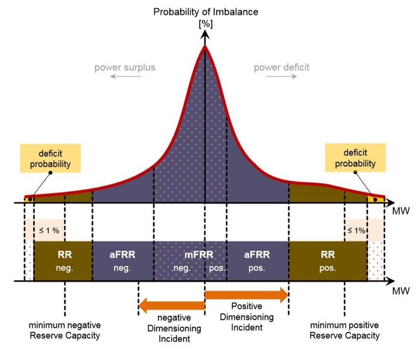
Table of Contents

1. Introduction .................................................................... 5
2. Model Structure and Optimisation Process .......................... 7
 2.1. Model Structure ................................................................................ 7
 2.2. Asset Library .................................................................................... 7
 2.3. Granularity, Horizons, and Objective Function ...................................... 8
 2.3.1. General Structure of the optimization problem ..................................... 8
 2.3.2. Horizons and optimisation Process ...................................................... 9
3. Asset Models ................................................................. 11
 3.1. Flexible assets: Cluster models ..........................................................11
 3.1.1. Cluster Model description ..................................................................11
 3.1.2. Notations ........................................................................................11
 3.1.3. Mathematical Modelling ....................................................................12
 3.1.4. Fleet Models ....................................................................................13
 3.1.5. Flexible assets technical parameters ..................................................13
 3.2. Hydro-power and storage..................................................................15
 3.2.1. Generic hydro storage model ............................................................15
 3.2.2. Inter-seasonal storage management ..................................................16
 3.3. Non-dispatchable assets ...................................................................17
 3.4. Reserve supply models .....................................................................19
 3.4.1. Reserve procurement methodology ....................................................19
 3.4.2. Reserve Types .................................................................................19
 3.4.3. Notations ........................................................................................20
 3.4.4. Constraints .....................................................................................21
4. Main Outputs And Visualization In The Interface ................ 23
 4.1. Main Key Performance Indicators .......................................................23
 4.2. Main Other Display Features ..............................................................23
5. Scenarios used in Metis Power System Models ................... 25
 5.1. Scenarios Available In METIS ............................................................25
 5.2. Standard Configuration of METIS .......................................................25
6. Appendix – Demand and RES data generation ................... 26
 6.1. Overall approach for climatic scenarios ...............................................26
 6.2. Demand profiles ..............................................................................26
 6.2.1. Temperature sensitivity and demand modelling ...................................26
 6.3. RES generation profiles.....................................................................27
 6.3.1. Generation of solar and onshore wind power profiles ............................27
7. Appendix – Reserve Sizing Methodology ........................... 31
 7.1. Main assumptions ............................................................................31
 7.2. Frequency Containment Reserve ........................................................31
 3

7.3. Automatic Frequency Restoration Reserve (aFRR) and Manual Frequency
 Restoration Reserve (mFRR) ...........................................................................32
 7.3.1. Units participating to the reserve .......................................................32
 7.3.2. Sizing approach ...............................................................................33
 7.3.3. Reserve sharing ..............................................................................38
8. References.................................................................... 41

 4

1. INTRODUCTION
METIS is an on-going project1 initiated by DG ENER for the development of an energy
modelling software, with the aim to further support DG ENER’s evidence-based policy
making, especially in the areas of electricity and gas. The software is developed by
Artelys with the support of IAEW (RWTH Aachen University), ConGas and Frontier
Economics as part of Horizons 2020 and is closely followed by DG ENER. METIS first
version was delivered at the DG ENER premises in February 2016.
The intention is to provide DG ENER with an in-house tool that can quickly provide
insights and robust answers to complex economic and energy related questions, focusing
on the short-term operation of the energy system and markets. METIS was used, along
with PRIMES, in the impact assessment of the Market Design Initiative.

 Figure 1: METIS models displayed in the Crystal Super Grid user interface
The Power System Module of METIS has been designed to address multiple power
systems problematics, following a welfare-maximization principle. It can be used to
analyse the European power systems’ dynamics, by providing production plans,
electricity flows, production costs, systemic marginal costs, scarcity periods and loss of
load, or other standard indicators detailed further in the document.
Such a modelling tool can be used to conduct different types of studies or quantitative
analysis on power systems, among which:
  Generation adequacy analysis,

  Impacts of Renewable Energy Sources integration on the energy system and
 market functioning,

  Cost-benefit analysis of infrastructure projects, as well as impacts on security of
 supply,

  Electricity flows between zones
  Impact of new energy usages (e.g. electrical vehicles, demand response) on the
 network reinforcement and generation costs,

1
 http://ec.europa.eu/dgs/energy/tenders/doc/2014/2014s_152_272370_specifications.pdf

 5

 Impact of day-ahead market measures such as rules for reserve sizing or
 participants in reserve procurement.

The present document is organised as follows:
  Section 2 is dedicated to the description of the general structure of the model,
 the optimisation problem it implements, and the way it is solved,

  Section 3 focuses on the specification of the asset models, going in depth into
 cluster and reserve models,

  Section 4 describes briefly the main visualization features to display results of
 the METIS Power System Module,

  Section 5 recalls the scenarios that are implemented and summarizes the main
 assumptions for the models that have been delivered to the European
 Commission.
  Three appendixes are also available, detailing technical parameters of assets,
 demand and RES data generation, and the reserve sizing methodology.

Note that METIS also embeds a Gas System Module (allowing to model the European gas
system) and a Power Market Module (containing models for European intra-day and
balancing markets) which have their own specific documentation. A demand and a gas
market module are also currently in development (as of May 15, 2017).

 6

2. MODEL STRUCTURE AND OPTIMISATION PROCESS
2.1. MODEL STRUCTURE
In METIS, the power system is represented by a network in which each node stands for a
geographical zone2 that can be linked to other zones with power transmissions. At each
node are attached assets that represent all consumption and production of energy at this
node. The model aims at minimizing the overall cost of the system to maintain a
supply/demand equilibrium at each node, at an hourly time step.
While the typical METIS models are at country-granularity, zones can also be configured
to stand for either NUTS2 zones or for aggregations of country, depending on the needs
of the study.
The following sections describe the list of assets included in the model, and specify the
main characteristics of the optimisation problem built from the model and of its solving
method.

2.2. ASSET LIBRARY
METIS Power System Module contains a library of assets for production, consumption and
transmissions that can be attached to each node of the network. The following assets are
included:
  Thermal non-RES assets

  Nuclear: power generation using nuclear technology,
  Lignite: power generation using lignite as primary fuel,
  Coal: power generation using coal as primary fuel,
  CCGT (gas): power generation, with combined cycles, using gas as primary fuel,
  Oil: power generation using diesel as primary fuel,
  OCGT (gas): power generation using gas as primary fuel,
  Derived gas: power generation using derived gas a fuel,
  Hydro assets

  Hydro-reservoir: hydro power generation associated with a storage capacity, water
 inflows and an optional pumping capacity (for mixed PHS),
  Hydro run-of-the-river: intermittent power generation using run of river turbines,
  Pure pumped hydro storage: pumped hydro storage without natural hydro inflows.
  Other RES assets

  Onshore and offshore wind power: intermittent power generation, based on wind
 scenarios,
  Solar fleet: intermittent power generation, based on solar irradiation scenarios
  Geothermal power: intermittent power generation
  Biomass/Waste fleet: power generation, using biomass/waste as fuel
  Other RES: intermittent power generation, corresponding to all other RES (includes
 Tidal power)
  Other storage assets

2
 Depending on the spatial granularity, a zone may be a subnational region, a country, a set of countries
aggregated into one, etc.
 7

 Batteries
  Compressed air energy storage
  Power Consumption: represent the aggregated consumption of electricity at this
 node.
  Power transmission: represent the power exchange capacity between two nodes.
 If zones correspond to European countries, the power transmission between two
 nodes represents the NTC capacity,

  Fuel contracts: represent the fuel purchase contracts (taking into account the fuel
 price) for thermal power assets,

  Water inflow: represent the water inflows for hydro-reservoirs,

  Total CO2 emissions: represent the total CO2 emissions of thermal assets,
 associated with a CO2 price,

  Reserve requirements: represent the needs for reserve at each node. Used only
 for models with reserve.

  Loss of load: represents the load curtailment that is done at a node as a last
 recourse if demand is higher than production, at a very high price (VoLL).

  Well: represents the surplus of energy at a node that happens when production is
 higher than consumption.

2.3. GRANULARITY, HORIZONS, AND OBJECTIVE FUNCTION

2.3.1. GENERAL STRUCTURE OF THE OPTIMIZATION PROBLEM
Simulations of the power system in METIS are performed with Artelys Crystal
Optimisation Engine and aim at determining a cost-minimizing production plan that
ensures a supply /demand equilibrium at each node over the study period, at an hourly
time step. This is done by solving an optimisation problem whose characteristics are
described below.
The electricity3 supply-demand equilibrium constraint at each node and each
time step is the following:
 , = , 
with

 , = ∑ , + ∑ ′ → , + 
 ℎ ′ 
 
 , = ∑ , + ∑ → ′, + 
 ℎ ′ 
 
In country-granularity models, consumers at node n are limited to a national
consumption plus the consumption of pumped hydro storages.
The objective function of the system is the total cost of the system:

 = ∑ + + 
 
3
 If the model takes into account reserves, supply/demand equilibrium constraints are set for each reserve type.
The objective function remain the same but additional constraints are set on producers, which usually increases
the overall costs of the system. More details on reserve constraints are given in section 0.
 8

Where:
  represent the production costs of the producer p, including fuel
 costs, CO2 costs, Variable OPEX 4. Fixed annual CAPEX and OPEX can also be
 considered if relevant.
  represent the costs associated to loss of load, computed as the
 product between the total loss of load (across all zones and all time steps) and the
 value of lost load (VoLL), usually 15 k€/MWh.
  represent the costs associated to the fact of having surplus energy in
 some zones, which can be penalised proportionally to the total volume of surplus.

2.3.2. HORIZONS AND OPTIMISATION PROCESS
METIS models are simulated by performing an optimisation of the production plan over a
year, at an hourly time step. This can reveal to be quite complicated as the typical
European model has around 30 assets by country and 34 countries, and can be even
more complicated with models at NUTS2 geographical granularity.
For that purpose, the optimisation problem is solved using a rolling horizon approach.
The solution of for the whole period is obtained by solving iteratively smaller problems as
depicted in Figure 2.
Three horizons are defined:
  The strategic horizon corresponds to the full duration of the entire problem,

  The tactical horizon corresponds to the length of the smaller optimisation
 problems horizon,

  The operation horizon corresponds to the length of the interval for which the
 solutions of the small optimisation problem are kept in the full solution.

 Figure 2: Optimisation process used to simulate METIS models

The resolution consists in solving successive simulation problems over a tactical horizon.
The solution kept over each iteration is defined by the operational horizon. At each
iteration, the initial states of the assets are set using results obtained from the previous

4
 See section 0 for more details.
 9

iteration (states of the assets at the end of previous operational horizon). Figure 2 and
Figure 3 describe the simulation procedure and how results are generated.

 Figure 3: Extraction of final results using the intermediate problems solutions
For the standard METIS European power system model, the strategic horizon corresponds
to one year. The tactical horizon is usually set to 15 days and the operational horizon to
7 days. The durations of tactical and operational horizon can also be modified if needed,
depending on the user needs. However, since these values have been chosen to balance
computational accuracy and computation time, it is advised to keep them unchanged. For
instance, increasing the tactical horizon can make the overall solution very anticipative.

 10

3. ASSET MODELS
This section describes the main assumptions used to model power generation technical
constraints. Each asset of the library given in section 2.2 has a specific asset model:
  Demand assets (power and reserve) are modelled with demand time series,
 which have to be satisfied at each time,
  Intermittent power generation are modelled with a time series curve
 corresponding to its maximum possible generation, a variable production cost
 (usually very cheap) and a possible penalty for curtailment (proportional to the
 energy curtailed),
  Thermal power generation (renewable and non-renewable) are usually
 modelled with cluster and reserve models described in section 3.1,
  Hydro assets and storages are also modelled with cluster models and other
 specific assets, as described in section 3.2,
  Loss of load assets are modelled as an electricity producer with an unlimited
 capacity and a variable cost of VoLL.
These models are described in more details in the following sections.

3.1. FLEXIBLE ASSETS: CLUSTER MODELS

3.1.1. CLUSTER MODEL DESCRIPTION
In METIS, units of the same technology or using the same fuel in each zone are bundled
together into the same asset. Thermal technologies such as Coal, CCGT, Lignite, OCGT
are also divided in three assets corresponding to units built before 1999, between 2000
and 2015, and after 2015.
Thermal production and storage units are subject to dynamic constraints such as ramping
gradients, minimal generation load, starting costs or minimal durations after turning
them off during which they have to be kept off before turning them on again.
These constraints are often taken into account with a unit-by-unit modelling, which is
computationally incompatible with a European optimal dispatch of the system. For that
purpose, METIS uses so-called cluster models which allow to take into account dynamic
constraints and starting costs in a relaxed (LP) unit commitment, without having to
include any binary variables, hence avoiding excessively increasing the problem
complexity.
In addition to the variables for generation at each time step, the cluster model introduces
new variables representing the capacity of running units of each cluster at each time
step. The generation variable of an asset is then bounded by its running capacity. The
constraints are described in details below.

3.1.2. NOTATIONS

Parameters
For each cluster , at each time step :

  : Generation cost (€/MWh), Cost to generate 1 MWh of electricity.
 This cost includes variable OPEX, fuel and CO2 costs.

  ̅ : Running cost (€/MW/h), Cost to have 1 MW of running capacity (independent
 
 from their load level).
 Generation and running costs are computed using efficiency data at Pmin and
 Pmax by type of unit (see section 3.1.5), to represent the lower efficiency of
 partially loaded units

 11

 : Start-up cost (€/MW),

  : Installed capacity of the asset (MW)

  : Minimum stable generation (%), as a proportion of the running
 capacity

  , : Availability (%), as a proportion of the installed capacity of the asset

  : Minimum off-state duration (number of time steps ≥ 1)
 
Variables
For each asset , at each time step :

  , [MW]: Generation variable (≥ 0)

  ̅ , [MW]: Running capacity variable (≥ 0)
 
  Difference variables:
 o ̅+
 , [MW]
 Positive part of difference in running capacity between t-1 and t (≥ 0).
 Constraints linking ̅+ ̅
 , to , are detailed below.

 o ̅−
 , [MW]
 Positive part of the shutdown power between t-1 and t (≥ 0)

  ̃ , [MW]: Capacity of off-state units which could be started-up (≥ 0)
 
 ̅ + represents the capacity that has been started at time step t.
The difference variable , 
Start-up costs are associated with this variable.
 ̅ − , it represents the capacity that has been shut down at time step t. It will be
As for , 
used to determine power which could be started-up ̃ , . Indeed, ̃ , is the capacity which
is turned off at time step t and which was shut down more than time steps before
time step t.

3.1.3. MATHEMATICAL MODELLING

Costs
With these notations the following costs can be defined:

  Generation costs: ⋅ , 
  Running costs: ̅ ⋅ ̅ , 
  Start-up costs: ⋅ , ̅+

The overall cost associated with a cluster for a given solution of this cluster’s decision
 ̅ + ) is the sum those costs:
variables at time step ( , ; ̅ , ; , 

 ̅ ⋅ 
 , = ⋅ , + ̅+
 ̅ , + ⋅ , 

 ̅ − and ̃ , does not have associated costs, however they are linked to
Note that variables , 
costly decision variables , , ̅ , and , ̅ + through constraints (see next paragraph)
impacting all variables’ dynamics and therefore the overall cluster cost.

Constraints
 12

A thermal cluster is subjected to the following constraints:
  Generation bounded by running capacity:

 ̅ , 
 , ≤ 

  Running capacity bounded by available installed capacity:

 ̅ , ≤ ⋅ , 
 
  Minimum stable generation constraint:

 ̅ , ≤ , 
 ⋅ 

  Difference variables:
 ̅+
 ̅ ̅
 , ≥ , − , − 

 ̅−
 ̅ ̅
 , ≥ , − − , 

 ̅+
 ̅− ̅ ̅
 , − , = , − , − 

  Minimum off-state duration

 ̃ , = 
 ̅+
 ̃ , − − ̅−
 , + , + − + ⋅ ( , − , − )
 
3.1.4. FLEET MODELS
When it is not necessary to represent the dynamic constraints of a given asset, one
might decide to use a fleet model instead of cluster model. The fleet model is a
simplification of a cluster model, as the only variable of the asset is the generation level
at each hour. The only remaining costs and constraints are:
  , ≤ ⋅ , 
  , = ⋅ , 

If relevant, it is also possible to set a minimum generation constraint, e.g. to force an
asset to be in must-run throughout the year, or gradient constraint to limit the variation
of generation between two consecutive time steps.

3.1.5. FLEXIBLE ASSETS TECHNICAL PARAMETERS
A literature review [3-16] resulted in the technical characterization of the different fleets
shown below. Characteristics include minimum stable generation (in % of ),
minimum off-state duration (also used as minimum start-up time in Intraday models
(c.f. Technical Note T2), maximum gradient, start-up costs.
Efficiency values at several operating points, and an average value were also provided by
[14]. Moreover, for each fleet, the article provides a function which adjusts efficiency to
the building year of the unit.

 13

In the following Table, “oldest” corresponds to units built before 2000 5, “prevailing”
 before 2015 and “state of the art” after 2015.

Parameters \ Minimal Positive Negative Starting Off-state Efficiency
 Type of unit generation load load cost minimal (%)
 level (% of gradient gradient (€/MW) duration @Pmin/@P
 Pmax) (% of (% of (h)6 max
 Pmax) Pmax)
OCGT - 50% 8%/min 8%/min 30

3.2. HYDRO-POWER AND STORAGE
Run-of-river power plants, inter-seasonal storage dams/reservoirs and pumped hydro
storage units are modelled separately.
Run-of-river power plants are represented as uncontrollable (non-dispatchable)
generation assets, which means that their generation at all times is determined by a load
factor time series.
Hydro-reservoir represents hydraulic dams which have a storage capacity, a natural
inflows and extra constraints due to long-term storage management, and an optional
pumping capacity.
Pure pumped hydro storage can also be modelled as storage assets, with an overall
efficiency of 81% (see next paragraph).
In the paragraphs below, we describe the generic hydro storage model used in METIS,
and how are handled long-term storages in typical simulations.

3.2.1. GENERIC HYDRO STORAGE MODEL
Storage assets are defined by:
  A storage capacity which represents the maximal energy volume that can be
 stored,
 
  A maximum input capacity which represents the maximum amount of energy
 the asset can receive from the power system to store during one hour,
 
  A maximum output capacity which represents the maximum amount of
 energy the asset can inject into the power system during one hour, using its
 storage capacity,
  Efficiency rates and which represent losses occurring when
 storing/injecting energy from/to the power system,
  A water inflow time series , which represents the optional water inflow
 for hydro-reservoir,
  An availability time series , which varies in the [0,1] interval and
 represents if the production or consumption capacities are unavailable (e.g. in
 maintenance).
The storage dynamics is given by:
 1
 ∀ , +1 = + + ⋅ − 
 
With input and output power being subjected to:
 0 ≤ ≤ 
 OUT
 ∙ 
 
 0 ≤ ≤ ∙ 
Moreover, the total stored volume at a given date cannot exceed the storage capacity:
 ∀ , 0 ≤ ≤ 
The storage capacity is often characterized by its discharge duration, which can be
computed using the following relation:
 
 ℎ = ⋅ 
 
 15

Member State Pumping capacities (MW) Member State Pumping capacities (MW)
 Mixed Pure Mixed Pure
 Austria 5661 0 Italy 3598 3957
 Belgium 0 1310 Latvia 0 0
 Bulgaria 149 864 Lituania 0 760
 Croatia 293 0 Luxembourg 0 1300
 Cyprus 0 0 Malta 0 0
 Czech Republic 0 1172 Netherlands 37 0
 Denmark 0 111 Poland 376 1606
 Estonia 0 46 Portugal 4004 0
 Finland 0 0 Romania 269 92
 France 5393 1793 Slovakia 0 916
 Germany 1633 7448 Slovenia 0 180
 Greece 1751 0 Spain 2786 3380
 Hungary 0 0 Sweden 0 235
 Ireland 146 292 United Kingdom 0 2682

 Table 2: Hydro pumping capacities in Europe (source: PRIMES)

3.2.2. INTER-SEASONAL STORAGE MANAGEMENT
Storages assets have a limited energy volume that can be injected in the network in a
given time range. In the case of hydraulic dams this limit is typically annual and given by
the total water inflow over the year. It usually prevents storage plants from constantly
generating power at full capacity. As a consequence, the water stored in dams has to be
saved when it is not most needed to produce electricity during more demanding periods.
Such an economic-based management, applied to hydro dams at different time scales –
from weekly to inter-seasonal, has to be enforced in METIS due to the rolling
optimization horizons. It is done in the system module by setting a guide curve9 which
defines, on a weekly basis, the minimal allowed storage level. The storage level time
series resulting from METIS Power System Module therefore takes into account both mid-
term water management (by satisfying the weekly “guide” curve) and short-term
management (through the hourly optimization).

9
 This curve, based on historical data, actually takes into account non-economic – or non-modelled –
considerations (such as tourism or agricultural needs), that affect water management.
 16

3.5

 3

 2.5
 Energy volume (TWh)

 2

 1.5

 1

 0.5

 0

 Minimal storage level allowed Actual storage level

 Figure 4: Illustrative inter-seasonal storage management replicated in METIS
 (France in standard climate conditions)

3.3. NON-DISPATCHABLE ASSETS
Non-dispatchable generation (Wind, Solar, run-off-river, etc.) are modelled as a single
asset by country and by type of technology. Every asset is defined by a variable cost that
depends on the technology, and an availability time series. Depending on the market
configuration, non-dispatchable assets may be curtailable and may be able to provide
upwards and downwards reserves. Biomass is modelled as a wood utility and is either
must-run or flexible depending on the market context. More information is available in
Technical Note T2.

 PV Wind Wind Run-of- Waste Derived Geothermal
 onshore offshore the- gasses
 river
Variable 0 0.5 0.5 0 3.7 3.5 0.32
cost
(€/MWh)
Availability Hourly time series Monthly Fixed Fixed Fixed
 time
 series
 Table 3 – Non-dispatchable assets’ parameters
 Source: PRIMES

CHP units are not modelled per se10, but are included in the thermal (coal, gas and
biomass) capacities.

Ten years of weather data have been used to build a database of hourly generation for
PV, onshore and offshore wind. The mean load factors by country for PV, onshore and
offshore wind are based on PRIMES EUCO27 data.

EMHIRES11 datasets of hourly wind and solar power capacity factor have also been
integrated in the METIS database.

10
 METIS Heat Module is planned for 2017-2018 and will include CHP units.
 17

Zone year 2001 year 2002 year 2003 year 2004 year 2005 year 2006 year 2007 year 2008 year 2009 year 2010
 SC8 SC9 SC10 SC1 SC2 SC3 SC4 SC5 SC6 SC7
 AT 2 364h 2 271h 2 121h 2 251h 2 225h 2 154h 2 354h 2 273h 2 226h 2 254h
 BA 2 409h 2 266h 2 142h 2 230h 2 042h 1 987h 2 138h 2 217h 2 151h 2 325h
 BE 2 456h 2 513h 2 157h 2 401h 2 268h 2 483h 2 558h 2 520h 2 364h 2 165h
 BG 2 827h 2 607h 2 459h 2 657h 2 647h 2 468h 2 610h 2 541h 2 361h 2 593h
 CH 1 369h 1 277h 1 207h 1 284h 1 165h 1 250h 1 294h 1 303h 1 269h 1 260h
 CZ 2 013h 2 118h 1 869h 2 161h 2 011h 1 951h 2 321h 2 116h 1 957h 1 945h
 DE 1 612h 1 693h 1 455h 1 679h 1 550h 1 622h 1 832h 1 731h 1 580h 1 471h
 DK 2 464h 2 642h 2 399h 2 697h 2 646h 2 494h 2 876h 2 791h 2 586h 2 487h
 EE 2 171h 2 130h 2 225h 2 139h 2 265h 2 211h 2 350h 2 567h 2 015h 2 046h
 ES 2 722h 2 629h 2 540h 2 417h 2 480h 2 470h 2 452h 2 521h 2 604h 2 704h
 FI 2 638h 2 408h 2 690h 2 519h 2 773h 2 603h 2 754h 2 764h 2 447h 2 402h
 FR 2 626h 2 652h 2 350h 2 473h 2 411h 2 496h 2 602h 2 541h 2 444h 2 427h
 GR 2 970h 2 433h 2 882h 2 778h 2 757h 2 784h 2 720h 2 802h 2 730h 2 728h
 HR 1 919h 1 778h 1 779h 1 765h 1 703h 1 653h 1 716h 1 776h 1 789h 1 795h
 HU 2 031h 1 960h 1 808h 1 873h 1 859h 1 665h 1 882h 1 903h 1 781h 1 874h
 IE 2 611h 3 022h 2 862h 2 973h 2 936h 2 908h 2 822h 3 095h 2 928h 2 340h
 IT 2 241h 2 035h 2 097h 2 145h 2 045h 1 946h 2 120h 2 105h 2 203h 2 235h
 LT 1 842h 2 002h 1 916h 1 875h 1 759h 1 758h 2 015h 2 093h 1 746h 1 783h
 LU 1 815h 1 832h 1 581h 1 724h 1 571h 1 743h 1 853h 1 750h 1 654h 1 558h
 LV 2 379h 2 510h 2 473h 2 424h 2 392h 2 383h 2 643h 2 800h 2 328h 2 300h
 ME 2 436h 2 216h 2 281h 2 353h 2 128h 2 025h 2 185h 2 227h 2 209h 2 396h
 MK 1 134h 1 013h 1 076h 1 165h 1 064h 938h 1 044h 1 073h 1 035h 1 163h
 NL 2 514h 2 580h 2 251h 2 595h 2 505h 2 623h 2 786h 2 810h 2 558h 2 303h
 NO 2 488h 2 446h 2 533h 2 667h 2 843h 2 684h 2 839h 2 681h 2 665h 2 321h
 PL 2 100h 2 252h 2 045h 2 213h 2 038h 1 953h 2 359h 2 261h 1 986h 2 093h
 PT 2 851h 2 755h 2 639h 2 429h 2 571h 2 532h 2 436h 2 592h 2 645h 2 848h
 RO 2 684h 2 646h 2 471h 2 597h 2 502h 2 413h 2 634h 2 538h 2 305h 2 523h
 RS 1 558h 1 522h 1 346h 1 501h 1 389h 1 262h 1 393h 1 464h 1 349h 1 550h
 SE 2 678h 2 606h 2 708h 2 754h 2 788h 2 664h 2 918h 2 832h 2 608h 2 560h
 SI 1 612h 1 424h 1 414h 1 371h 1 400h 1 402h 1 469h 1 480h 1 481h 1 498h
 SK 1 439h 1 434h 1 315h 1 390h 1 351h 1 212h 1 430h 1 428h 1 280h 1 345h
 UK 2 564h 2 694h 2 568h 2 766h 2 867h 2 730h 2 794h 2 965h 2 736h 2 319h

 Table 4 - Wind onshore generation yearly full load hours (for the different years of weather data)

 Zone year 2001 year 2002 year 2003 year 2004 year 2005 year 2006 year 2007 year 2008 year 2009 year 2010
 SC8 SC9 SC10 SC1 SC2 SC3 SC4 SC5 SC6 SC7
 BE 3 501h 3 505h 3 114h 3 342h 3 305h 3 535h 3 585h 3 630h 3 359h 3 158h
 DE 3 187h 3 362h 3 028h 3 407h 3 412h 3 265h 3 640h 3 643h 3 351h 3 160h
 DK 4 129h 4 355h 4 047h 4 389h 4 282h 4 145h 4 480h 4 379h 4 331h 4 190h
 EE 2 131h 2 031h 2 157h 2 078h 2 182h 2 162h 2 309h 2 525h 1 946h 2 001h
 ES 2 998h 2 946h 2 604h 2 641h 2 902h 2 759h 2 655h 2 509h 2 753h 3 052h
 FI 2 990h 2 583h 2 952h 2 834h 3 018h 2 866h 3 022h 2 988h 2 711h 2 626h
 FR 3 255h 3 357h 3 011h 3 051h 3 016h 3 151h 3 225h 3 228h 3 025h 3 002h
 IE 3 037h 3 466h 3 320h 3 423h 3 462h 3 374h 3 262h 3 546h 3 435h 2 787h
 IT 3 466h 3 067h 3 117h 3 182h 3 066h 2 827h 3 099h 3 176h 3 215h 3 473h
 LV 3 001h 3 306h 3 071h 3 266h 3 076h 3 048h 3 332h 3 461h 3 064h 3 037h
 NL 3 614h 3 578h 3 256h 3 601h 3 588h 3 699h 3 852h 3 920h 3 649h 3 355h
 PL 2 989h 3 201h 2 970h 3 237h 2 942h 2 843h 3 327h 3 272h 2 936h 3 013h
 PT 2 859h 2 936h 2 591h 2 480h 2 776h 2 690h 2 528h 2 447h 2 633h 2 977h
 SE 2 813h 3 036h 2 848h 3 068h 2 939h 2 811h 3 195h 3 148h 2 952h 2 890h
 UK 2 968h 3 064h 2 931h 3 038h 3 112h 3 103h 3 116h 3 322h 3 020h 2 722h

 Table 5 - Wind offshore generation yearly full load hours (for the different years of weather data)

11
 EMHIRES datasets are an initiative from the Joint Research Centre of the European Commission. More
information is available in [25].
 18

Zone year 2001 year 2002 year 2003 year 2004 year 2005 year 2006 year 2007 year 2008 year 2009 year 2010
 SC8 SC9 SC10 SC1 SC2 SC3 SC4 SC5 SC6 SC7
 AT 1 102h 1 100h 1 231h 1 128h 1 150h 1 139h 1 144h 1 105h 1 114h 1 069h
 BE 1 022h 1 038h 1 157h 1 073h 1 080h 1 062h 1 033h 1 023h 1 072h 1 065h
 BG 1 327h 1 302h 1 353h 1 324h 1 271h 1 305h 1 343h 1 335h 1 302h 1 255h
 CH 800h 785h 898h 850h 837h 844h 839h 807h 839h 782h
 CZ 895h 934h 1 056h 971h 994h 987h 967h 950h 955h 923h
 DE 919h 931h 1 058h 967h 987h 977h 938h 951h 969h 947h
 DK 894h 916h 947h 915h 922h 918h 893h 930h 933h 905h
 EE 821h 913h 824h 816h 866h 876h 840h 797h 825h 818h
 ES 1 965h 1 936h 1 936h 1 973h 2 018h 1 955h 1 955h 1 911h 1 966h 1 900h
 FI 733h 808h 745h 729h 768h 785h 734h 714h 757h 728h
 FR 1 566h 1 554h 1 680h 1 621h 1 640h 1 605h 1 582h 1 551h 1 624h 1 582h
 GR 1 635h 1 586h 1 603h 1 616h 1 594h 1 586h 1 623h 1 610h 1 563h 1 557h
 HR 1 447h 1 409h 1 523h 1 398h 1 435h 1 438h 1 453h 1 429h 1 431h 1 363h
 HU 880h 901h 974h 893h 909h 902h 929h 900h 914h 856h
 IE 876h 843h 893h 873h 858h 865h 860h 831h 835h 893h
 IT 1 428h 1 356h 1 458h 1 402h 1 410h 1 427h 1 435h 1 385h 1 398h 1 336h
 LT 842h 895h 881h 855h 890h 888h 855h 833h 862h 846h
 LU 862h 883h 986h 916h 916h 893h 873h 863h 902h 896h
 LV 840h 898h 872h 851h 892h 896h 852h 829h 846h 838h
 MK 1 298h 1 266h 1 307h 1 285h 1 283h 1 288h 1 300h 1 297h 1 244h 1 209h
 NL 871h 872h 962h 898h 912h 901h 870h 881h 903h 895h
 PL 803h 851h 921h 868h 897h 885h 858h 852h 867h 834h
 PT 1 820h 1 792h 1 807h 1 876h 1 900h 1 837h 1 881h 1 829h 1 852h 1 800h
 RO 1 333h 1 337h 1 402h 1 344h 1 302h 1 332h 1 385h 1 361h 1 366h 1 283h
 RS 1 076h 1 088h 1 149h 1 081h 1 090h 1 092h 1 116h 1 109h 1 093h 1 028h
 SE 837h 883h 873h 857h 873h 863h 840h 854h 852h 835h
 SI 1 089h 1 064h 1 177h 1 056h 1 089h 1 083h 1 108h 1 061h 1 074h 1 018h
 SK 869h 903h 981h 908h 919h 923h 928h 902h 916h 864h
 UK 808h 796h 873h 801h 816h 827h 801h 798h 803h 811h

 Table 6 - PV generation yearly full load hours (for the different years of weather data)
More details on the methodology are given in the appendix in section 6.

3.4. RESERVE SUPPLY MODELS

3.4.1. RESERVE PROCUREMENT METHODOLOGY
It is possible to take into account reserve allocation in METIS models. In this case new
variables and constraints are added to the model presented in the previous sections. The
reserve allocation and power dispatch are then obtained simultaneously by solving an
optimisation problem minimizing costs to ensure a reserve and power supply/demand
equilibrium.
Note that in itself, the reserve allocation does not incur any direct costs as there is
usually no variable costs for allocating reserve capacity (since reserve activation is not
simulated). However, the additional constraints on assets to provide reserve might force
them to run at a less efficient generation level, incur additional start-up costs, or trigger
opportunity costs.

3.4.2. RESERVE TYPES
Unpredicted events, such as unplanned outages of power plants or forecast errors of load
or renewable energy generation, can result in imbalances of the power grid on different
time horizons. Different types of reserve, characterized by their activation delay, are
therefore procured in advance and then activated to restore balance on the power grid.
The Frequency Containment Reserve (FCR) aims at securing the grid’s security in case of
instantaneous power deviation (power plant outages, sharp load deviation, line section,
etc.). It is dimensioned by the maximum expected instantaneous power deviation and

 19

must be available within 30 seconds (see section 7), meaning that only synchronised
units (i.e. units that are currently running) can participate in FCR.
The Automatic Frequency Restoration Reserve (aFRR) and the Manual Frequency
Restauration Reserve (mFRR) have different activation times - 5 and 15 minutes will be
considered as standard for the aFRR and mFRR respectively. They can be called upon to
compensate load fluctuations or forecast errors. Only synchronised units can participate
in aFRR procurement. However, due to their low activation time, hydro assets, OCGTs
and Oil fleets can participate in mFRR procurement from standstill.
In METIS models, FCR and aFRR are aggregated into “synchronised reserve”. One may
refer to the appendix – Reserve Sizing Methodology for more information and
justification.

 Figure 5: Reserve types and usages
For the standard METIS simulations, rules for reserve dimensioning have been
standardised and provide as output an hourly requirement for reserve, based on demand
and RES generation forecasts12. More details are given on section 7.

3.4.3. NOTATIONS
The indexes i, j and t respectively refer to generation assets, reserve types and time
steps.
The notation ′ ≤ is used to indicate that reserve ′ has a shorter activation delay than
reserve .
  
 , , [MW]: participation of generation cluster in the upward reserve , at
 time step 

  
 , , [MW]: participation of generation cluster in the downward reserve ,
 at time step 

  
 , [MW]: upward reserve requirement at time step 

  
 , [MW]: downward reserve requirement at time step 

  : activation delay characterizing reserve 

  
 [MW/h]: maximum generation increase rate per hour (in % of running
 capacity)

12
 Forecast generation is described in detail in METIS Technical Note T2.
 20

 
 [MW/h]: maximum generation decrease rate per hour (in % of
 running capacity)

  
 , [%]: maximum acceptable share of running capacity to be allocated to
 upward reserves13. The value is zero if the asset is banned from upward reserve
 procurement.
  
 , [%]: maximum acceptable share of running capacity to be allocated to
 downward reserves14. The value is zero if the asset is banned from downward
 reserve procurement.

3.4.4. CONSTRAINTS
  Supply/demand constraint at all time for reserve
 
 ∀ , , ∑ , , = , 
 
 ∀ , , ∑ , , = , 
 
  Maximal participation in the primary and secondary reserves

A given cluster can only allocate a part of its running capacity to reserves, since starting
up more capacity would take longer than the available delay. The following constraints
apply to all clusters for primary and secondary reserves:

 , + ∑ , , ≤ ̅ , 15
 
 ⋅ ̅ , ≤ , − ∑ , , 
 16

 ∀ , , , 
 ∑ , ′, ≤ ̅ , ⋅ 
 , 
 ′ ≤ 

 ∀ , , , 
 ∑ , ′, ≤ ̅ , ⋅ 
 , 
 ′ ≤ 

  Maximal participation in the tertiary reserve

The tertiary reserve’s activation time may be long enough for peaking or hydro units to
start up and generate power within this delay 17. The following equations would then
apply to such clusters only:

 , + ∑ , , ≤ ⋅ , 
 
 0 ≤ , − ∑ , , 
 
 ∀ , , , ∑ , ′ , ≤ , ⋅ ⋅ , 

 ′ ≤ 

13
 For most thermal assets and for aFRR/mFRR, 
 , = ⋅ Δ 
 
14
 For most thermal assets and for aFRR/mFRR, , = ⋅ Δ 
15
 Note that this is a generalization of the constraint , ≤ ̅ , presented in the cluster model, which is implied
by the constraint presented here
16
 Note that this is a generalization of the constraint ⋅ ̅ , ≤ , presented in the cluster model, which
is implied by the constraint presented here
17
 A penalty is added to assets which supply tertiary reserve from standstill, to compensate start-up costs which
may occur if the asset is called for balancing services.
 21

 
 ∀ , , , ∑ , ′ , ≤ , ⋅ ⋅ , 
 ′ ≤ 

Other clusters (that is, clusters of which units which cannot start up fast enough) are
subject to the same maximal participation constraints for tertiary reserve as for the
primary and secondary reserves.
  Specific constraints for hydro storage plants

Storage clusters are subject to available energy constraints, in addition to generation
capacity constraints. The storage level of each storage asset is driven by the following
dynamics:

 1 
 ∀ , , , = , −1 + , + ⋅ , − , 
 
Where (or ) stands for input (or output) efficiency

Note that
 
  , = 0 for hydro dams without mixed pumping, which cannot consume electricity
 to fill their storage tanks,

  , = 0 for pure pumped hydro storage assets, which can only fill their
 reservoirs by activating their pumps.

Such dynamics imply that a storage plant cannot produce more energy than what is
stored (since the storage level has to be positive at all times):

 1
 ⋅ , ≤ , −1
 
Storages can participate in reserve procurement with their production component 18 as
long as the storage level is sufficient to generate reserve for Δ :

 1 
 ∀ , , Δ ∗ ∑ , , ≤ , 
 
 1 
 ∀ , , Δ ∗ ∑ , , ≤ ( − , )
 
In practice, the value of Δ depends on TSOs rules for storages’ reserve participation and
can vary from one TSO to the other. In METIS, we assume a value of 1h, thus allowing
the storage to participate in reserve as long as its storage level is enough to cover one
hour of reserve procurement.

  Reserve procurement from variable RES
Depending on the market configuration, variable renewable energy may participate in
reserve procurement. As variable RES and in particular wind energy have very high load
gradients and low minimum stable generation, the only constraints modelled are:
 
 , + ∑ , , ≤ ⋅ , 
 
 0 ≤ , − ∑ , , 
 
18
 It is assumed that pumped storages can only participate to reserve with their production component as their
consumption component (pump) usually runs at a fixed power level and thus cannot provide reserve.
 22

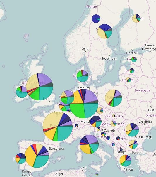
4. MAIN OUTPUTS AND VISUALIZATION IN THE INTERFACE
4.1. MAIN KEY PERFORMANCE INDICATORS
In addition to raw inputs and optimization results such as generation and running
capacities time series for each asset or flow of interconnection, the Crystal Super Grid
platform provides functionalities to display model parameters and aggregated results of
different assets in an ergonomic view using tables, charts or geographical display
functions. The main way to display this aggregated data are the Key Performance
Indicators whose full list and equations are detailed in the METIS KPI documentation.
The following KPIs are among the most useful (non-exhaustive list):
  Based on input data: Demand, reserve sizing, installed capacities, import
 capacity, import capacity over net demand,
  Based on optimisation results: Production and production costs by asset or
 aggregated at zone level, annual flows and congestion rent for interconnections,
 production curtailment and loss of load in each zone, marginal costs by zone and
 price divergence between zones, consumer, producer surplus and total welfare by
 zone,
KPIs can be displayed in tables or directly on the map view as shown in the following
figure:

 Figure 6: Production by asset and by country, displayed directly on the European map in Artelys
 Crystal Super Grid

4.2. MAIN OTHER DISPLAY FEATURES
In addition to aggregated yearly figures (KPIs), it is possible to display time series in a
synthetized view to better understand the functioning of the system. In particular,
marginal costs and cumulative generation curve are of the most useful features.

 23

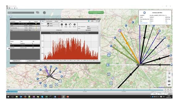
Figure 7: Cumulative generation curve for several days in Germany in 2050, simulated using METIS
 models and displayed in Artelys Crystal Super Grid

Productions - wind power (in turquoise and green), solar (in yellow), CCGTs (in purple) - are displayed
on top of each other, while demand is displayed with a red curve. Here, the production exceeds
demand during the whole period, meaning that the country exports electricity.
It is also possible to go more in depth of the functioning of a specific asset in the
production view, which is especially useful for cluster and reserve models, as it allows to
display in one chart the running capacity, generation level, minimal power and the 4
reserve allocations at each time step.

 Figure 8: Zoom on a coal fleet using METIS cluster and reserve model, in the production view of
 Artelys Crystal Super Grid

 24

5. SCENARIOS USED IN METIS POWER SYSTEM MODELS
5.1. SCENARIOS AVAILABLE IN METIS
In the version delivered to the European Commission, a METIS version of the PRIMES
scenarios has been implemented19:
  European Commission REF16 scenario (reference scenario published in 2016) for
 year 2020 and 2030
  European Commission EUCO30 scenario for year 2030 and 2050
  European Commission EUCO27 scenario for year 2030, used in particular for
 METIS S12 study on market design,
In addition to EU Member States, METIS scenarios include Switzerland, Bosnia, Serbia,
Macedonia, Montenegro and Norway to model the impact of power imports and exports
on the MS.
METIS versions of PRIMES scenarios include refinements on the time resolution (hourly)
and unit representation (explicit modelling of reserve supply at cluster and MS level).
Data provided by the PRIMES scenarios include: demand at MS-level, primary energy
costs, CO2 costs, installed capacities at MS-level, interconnection capacities. These
scenarios are complemented with METIS data such as consumption and RES generation
time series, availability time series for thermal fleets, unit technical data and constraints,
etc.
For that purpose, a specific document has been written on the integration of PRIMES data
into METIS for the construction of EUCO27 (METIS Technical Note T1). A similar approach
has been used for Ref16 and EUCO30 scenarios. Additionally, some details on Demand
and RES data generation are also available in the appendices (section 6).

5.2. STANDARD CONFIGURATION OF METIS
The scenarios delivered to the European Commission share by default the same
modelling options that are described briefly below:
  EU28 + 6 ENTSO-E non-EU countries are represented in the models, at a national
 granularity,
  Simulations are performed over a year, at an hourly time step, with an
 operational horizon of seven days and a tactical horizon of fifteen days,
  Models include reserve, with separated products for downwards and upwards
 reserve, a hourly reserve sizing20 done with a probabilistic approach and assuming
 a regional cooperation of countries,
  Reserve procurement is optimised jointly to the power dispatch,
  Thermal fleets are modelled as clusters with reserve,
  Biomass fleet is not considered as must-run, renewable fleets (Run-off-river,
 Biomass, Wind, Solar, Waste) can participate in reserve procurement, and there is
 no penalty for RES curtailment.
While these options correspond to the standard for these scenarios, the user can chose to
use other modelling options depending on the needs of the study.

19
 More information at https://ec.europa.eu/energy/en/data-analysis/energy-modelling
20
 More details in section 7 and METIS Technical Note T3.
 25

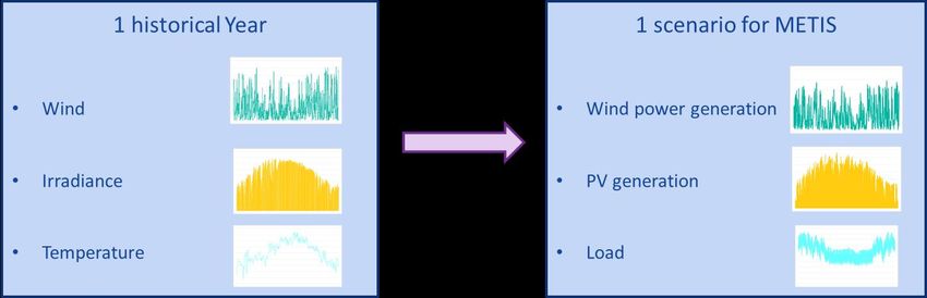
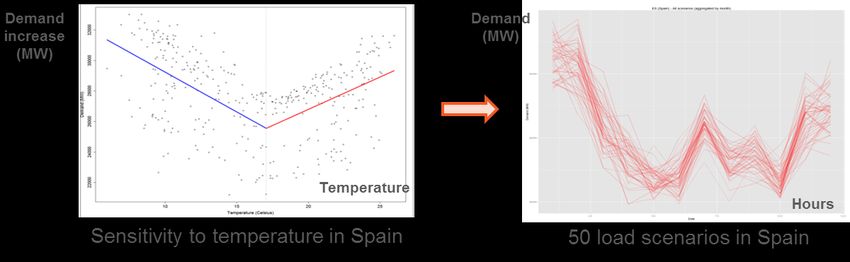
6. APPENDIX – DEMAND AND RES DATA GENERATION
6.1. OVERALL APPROACH FOR CLIMATIC SCENARIOS
To assess the benefits of regional cooperation, it is crucial to use consistent weather data
through Europe. For this reason, correlated RES generation data were integrated in
METIS, as represented in Figure 9.

 Figure 9: Correlated RES generation in METIS: for each year of weather data, one corresponding
 scenario is built.
The following paragraphs describe the methodology which was used to build the
correlated demand time series and RES generation.
RES generation and demand forecasts have also been generated for the Power Market
Module and for reserve sizing. The methodology for its computation is described in detail
in METIS Technical Note T2.

6.2. DEMAND PROFILES

6.2.1. TEMPERATURE SENSITIVITY AND DEMAND MODELLING
The objective is to generate fifty hourly scenarios of demand for each country by means
of a statistical model fitted to the following data sources:
  historical daily temperature data from years 1965 to 2014 for all countries
 from the European Climate Assessment & Dataset project (ECA), see [22].

  hourly demand data projections for 2030 provided by ENTSO-E TYNDP 2014 21
 visions 1 and 3, see [17].
In this regard, each demand scenario is modelled as the sum of a thermo-sensitive
component and the non-thermo-sensitive one. The thermo-sensitive component is
computed by using a piecewise linear model. This model is set up with one threshold and
two slopes22 and calibrated by getting recourse to a Multivariate Adaptive Regression
Splines method23 that involves the computation of temperature gradients (MW of demand
increase per °C increase) for each country.
As depicted in Figure 10 for Spain, the temperature scenarios of each country drive its
thermo-sensitive demand scenarios by using the country temperature gradients. Then,
thermo-sensitive and non-thermo-sensitive demand scenarios are added so as to
complete the generation of the country demand scenarios.

21
 Data is given as hourly time series for one year and average seasonal temperatures.
22
 The use of two slopes - one slope associated to low temperatures and one slope associated to high temperatures allows for
applying the same approach for each country, with the same number of parameters, although three slopes could have been
used for countries with both heating and cooling gradients.
23
 See [23] for the method and [24] for its R implementation.
 26

Figure 10: Two gradients and one threshold accounting for heating and cooling effects on Spain
 demand

6.3. RES GENERATION PROFILES

6.3.1. GENERATION OF SOLAR AND ONSHORE WIND POWER PROFILES
Generation of ten historical yearly profiles for wind power and solar power has been
performed by a model developed by IAEW. The model uses historical meteorological
data, units’ power curves and historical generation data as input parameters to
determine RES generation profiles and calibrate the results for each region in the models
scope.

The methodology is depicted in Figure 11.

 Input data Results

 Model

 meteorological data

 units’ power curve load factor time
 series for each
 aggregate meteorological use historical data for back country
 data for each country testing and calibrating model

 historical data

 Figure 11: Methodology

Input Data

Meteorological Data
The delivered time series of renewable feed-ins are based on fundamental wind, solar
and temperature time series for 10 years (2001 to 2010) on a detailed regional level
derived from the ERA-Interim data provided by Meteo Group Germany GmbH. From ERA-
Interim’s model, values for wind speed (m/s), global irradiation (W/m2) and temperature
(°C) are derived for every third hour and interpolated to hourly values by Meteo Group.
The regional resolution of the data is one hourly input series (wind, solar, temperature)
on a 0.75° (longitude) times 0.75° (latitude) grid model, which ensures an adequate

 27

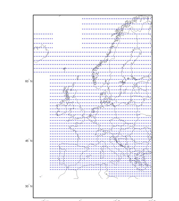
modeling accuracy. The regional resolution is shown in Figure 12, in which each blue dot
represents one data point.

 Figure 12: Regional resolution of meteorological data

Historical Data
To generate realistic time series, a calibration of the models is inevitable. Therefore
information regarding the yearly full load hours for wind and PV generation in each
country is necessary. To derive the yearly number of full load hours the installed
capacities of wind and PV generation as well as the yearly energy production have been
investigated for each country.
In case of unavailable data the full load hours were derived based on the data of a
neighboring country. As the availability for data regarding installed wind generation
capacities and generated energy is satisfying in almost every country it is rather low for
information regarding PV power. Only for a few countries reasonable full load hours could
be derived from historical published data. For the other country data from the
Photovoltaic Geographical Information System was used instead.

Model
In first step the high-resolution meteorological data are aggregated for each country and
NUTS2 region. The aggregation is thereby based on the regional distribution of wind and
PV capacities. The required distribution of wind and PV generation capacities is extracted
from different databases and is aggregated at high voltage network nodes. In countries
with no available information a uniform distribution is assumed.
Each high voltage network node gets the nearest meteorological data point assigned to
and the data is weighted with the installed capacity at the network node. Thereby the
wind-speed is weighted by the installed wind generation capacity whereas global
irradiation and temperature are weighted with the installed PV generation capacity. The
weighted time series for all nodes in each region are aggregated and divided by the
overall installed wind respectively PV capacities. Subsequently, it is necessary to calibrate
the generation models for each country by scaling the meteorological data accordingly.
The process of calibration is display in Figure 13.

 28

historical full load
 hours

 aggregated meteorological scaling of generation model load factor time
 data meteorological data series

 Figure 13: Model calibration
The meteorological data is fed into generation models for PV and wind generation. The
resulting load factor time series are compared with the historical full load hours for the
specific country and the deviation between load factor time series and the historic full
load hours in each year i is to be minimized by scaling the meteorological data
accordingly. In this minimization the yearly deviation between time series full load hours
(FLH) and historical data is weighted with the installed capacity (IC) in the specific year
according to formula 1.

 10

 min ∑( , − ,ℎ ) ∙ (1)
 =1

The scaling factors are chosen independently for wind speed and global irradiation and
are individual for each country.

Calibration to PRIMES load factors
In order to generate RES generation profiles for the METIS EuCo27 2030 scenario, the
installed capacities and full load hours for each country from PRIMES were used. From
these data each NUTS2 region was assigned a share of the country’s installed generation
capacities for PV, onshore wind and offshore wind (if applicable) according to the region’s
average global irradiation and wind speed in comparison to the countries average global
irradiation and wind speed, respectively. The model was then calibrated by minimizing
the deviation between time series full load hours and PRIMES full load hours in 2030.

The resulting full load hours for both wind and PV for exemplary countries are shown in
Figure 14.

 29

Figure 14 - Wind and PV full load hours per year
Whereas the PV full load hours per year are not changing significantly from one year to
the next, the resulting full load hours from wind generation vary considerably.

 30

7. APPENDIX – RESERVE SIZING METHODOLOGY
7.1. MAIN ASSUMPTIONS
One important assumption behind METIS modelling is that all markets are supposed to
be liquid. As such, the variations in net demand linked to the RES or demand forecast
errors up to t-1 are supposed to be met by the offers done on the intraday market. In
reality, TSOs use Replacement Reserves (RR), which are not explicitly modelled in the
system module24, to make sure that enough capacity is available and running (or ready
to be running) for the next 1 to 4 hours. Hence, only variations/events occurring in a
time horizon smaller than 1 hour are taken into account and used for the sizing of the
FCR, aFRR and mFRR.
Besides, METIS functions at an hourly granularity by default. As a consequence, 15 or
30 minutes intraday gateways are not modelled and all variations occurring inside the
hour have to be dealt with by the FRR.
Finally, FCR and aFRR are simulated as a single synchronized reserve and the specific
constraints of FCR are not integrated by default. FCR and aFRR sizing are added to define
the required synchronized reserve.
The main evolution in FRR needs that is to be assessed when comparing to today’s
situation is the growing share of renewables in the production mix. The immediate impact
will be that both empirical and deterministic methods (c.f. 7.3.2) which are currently
used in some countries will prove to be insufficient in the near/longer term, when
renewables account for an important part of the hourly/daily electricity production.
Reserve sizing is thus bound to evolve towards a more probabilistic approach.
In order to compute the FRR sizing following a probabilistic methodology, a TSO point of
view is used. It means a forecast state of the system, with a 5min granularity, is
compared to an actual state of the system, also with a 5min granularity. Reserves (aFRR
and mFRR) are called upon to take care of the resulting imbalances (difference between
what was forecast by the TSO and what actually happened). aFRR and mFRR sizings are
computed based on the 0.1% and 99.9% centiles of imbalances.
The whole simulation process and FRR sizing for typical METIS models is explained in
more details in the following parts.
Note that several options for reserve dimensioning are available and have been used for
the S12 study. They are described in details in Technical Note T3.

7.2. FREQUENCY CONTAINMENT RESERVE
FCR is shared between ENTSO-E continental members with a total sizing of 3GW which is
split among MS proportionally to their annual power generation. FCR sizing for each
Member State is assumed to follow the same rule up to 2030.
The FCR values used in METIS are presented below (FCR is assumed to be symmetrical
for each country).

24
 A proxy for RR is used in the Power Market Module, as is described in Technical Note T2.
 31

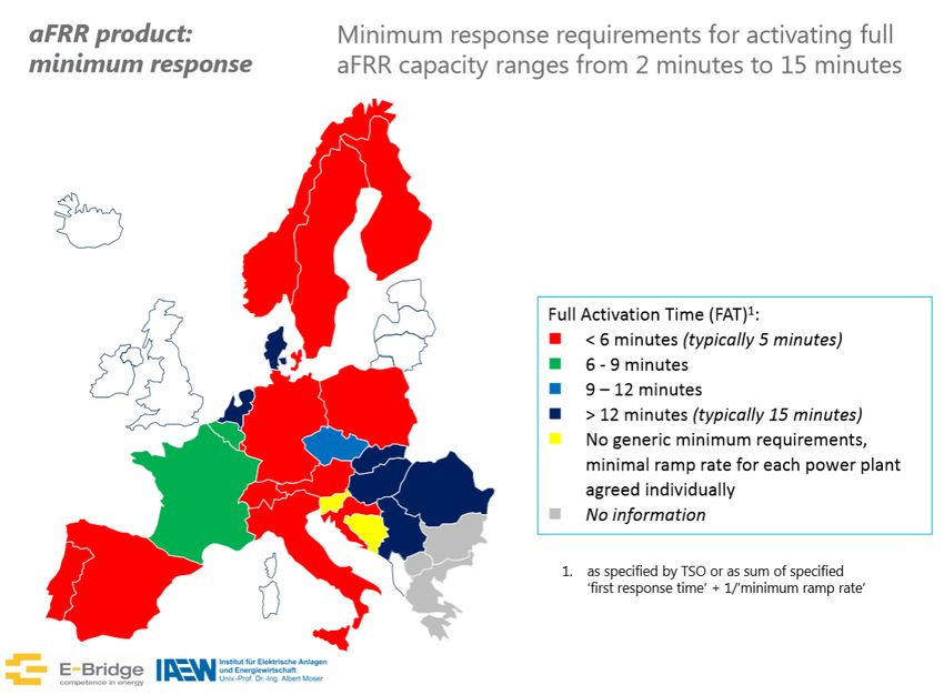
FCR FCR FCR FCR
 Country Country Country Country
 (MW) (MW) (MW) (MW)
 AT 65 EE 45 IT 535 PL 171
 BA 14 ES 421 LT 57 PT 51
 BE 100 FI 931 LU 6 RO 57
 BG 44 FR 650 LV 42 RS 46
 CH 71 GB 900 ME 25 SE 644
 CY GR 60 MK 9 SI 16
 CZ 75 HR 10 MT SK 29
 DE 583 HU 75 NL 102
 DK 50 IE 90 NO 352

 Table 7– FCR sizing by member state

7.3. AUTOMATIC FREQUENCY RESTORATION RESERVE (AFRR) AND MANUAL
 FREQUENCY RESTORATION RESERVE (MFRR)

7.3.1. UNITS PARTICIPATING TO THE RESERVE

Only synchronized units can participate in the aFRR because the Full Activation Time
(FAT), i.e. the time required for the reserve to be fully activated, is too low for the non-
synchronized units to start-up.
FAT varies a lot between Member States as can be seen on the following figure.

 32