Informing the planning of rotating power outages in heat waves through data analytics of connected smart thermostats for residential buildings
←
→
Page content transcription
If your browser does not render page correctly, please read the page content below
LETTER • OPEN ACCESS

Informing the planning of rotating power outages in heat waves through
data analytics of connected smart thermostats for residential buildings
To cite this article: Zhe Wang et al 2021 Environ. Res. Lett. 16 074003

View the article online for updates and enhancements.

                               This content was downloaded from IP address 46.4.80.155 on 10/10/2021 at 17:23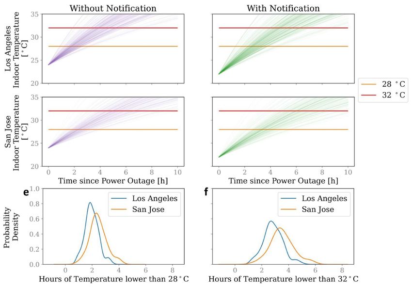
Environ. Res. Lett. 16 (2021) 074003 https://doi.org/10.1088/1748-9326/ac092f
LETTER
Informing the planning of rotating power outages in heat waves
OPEN ACCESS
through data analytics of connected smart thermostats for
RECEIVED
3 March 2021 residential buildings
REVISED
5 June 2021 Zhe Wang, Tianzhen Hong∗ and Han Li
ACCEPTED FOR PUBLICATION
Building Technology and Urban Systems Division, Lawrence Berkeley National Laboratory, One Cyclotron Road, Berkeley, CA 94720,
8 June 2021
United States of America
∗
PUBLISHED Author to whom any correspondence should be addressed.
22 June 2021
E-mail: thong@lbl.gov
Original content from Keywords: heat wave, power outage, building thermal dynamics, connected smart thermostat, hybrid inverse modelling
this work may be used
under the terms of the
Creative Commons
Attribution 4.0 licence.
Abstract
Any further distribution
of this work must With climate change, heat waves have become more frequent and intense. Rotating power outages
maintain attribution to
the author(s) and the title happen when the power supply is unable to meet the cooling demand increase resulting from
of the work, journal extreme high temperatures. Power outages during heat waves expose residents to high risks of
citation and DOI.
overheating. In this study, we propose a novel data-driven inverse modelling approach to inform
decision makers and grid operators on planning rotating power outages. We first infer the building
thermal characteristics using the connected smart thermostat data, and used the estimated thermal
dynamics to simulate the thermal resilience during a heat wave event. Our proposed method was
tested for the California power outage in August 2020 by using the open source Ecobee Donate
Your Data dataset. We found in California the power outage should not last more than two hours
during heat waves to avoid overheating risks. Informing the residents in advance so they can
prepare for it through pre-cooling is a simple but effective strategy to expand the acceptable power
outage duration. In addition to assisting power outage planning, the proposed method can be used
for other applications, such as to evaluate a building energy efficiency policy, to examine fuel
poverty, and to estimate the load shifting potential of building stocks.
1. Introduction electricity use for air conditioning. The atmospheric
warming in California is expected to increase grid
Heat waves happen when abnormally high outdoor peak demand in summer as much as 38% by the
temperature lasts for several days [1]. As one of many end of twenty-first century [10]. In August 2020,
consequences of climate change, heat waves have because of the region wide heat wave and unanti-
become more frequent and intense [2, 3]. During the cipated power supply shortage, California residents
past decade, extreme heat events have been recorded experienced rotating power outages.
in India [4], Russia [5], China [6], and many other The challenges posed by heat waves are more
places across the world. Heat waves are considered significant in cities for two reasons. First, climate
to be a critical public health threat, and they were change induced warming is more severe in cities
estimated to be responsible for the death of more than than their surrounding rural areas (i.e. the urban
70 000 people in the summer of 2003 in Europe [7] heat island effect); the difference could reach 4 ◦ C
and 55 000 people in Russia in 2010 [8]. With climate under a high-emission scenario [11]. Second, cool-
change, heatwave-related excess mortality is expected ing buildings accounts for a higher proportion of
to increase further, especially in tropical and subtrop- the total electricity demand in cities, compared to
ical countries and regions [9]. rural areas. If a power outage is unavoidable during
Meanwhile, extreme high ambient temperature heat waves, it is essential to understand how long it
drives up electricity demands and poses threats to could last, to prevent occupants from being exposed
grid reliability, because higher ambient temperat- to excess heat while the grid stress is being relieved.
ure leads to increased cooling loads and thus more Occupants’ exposure to excess heat indoors can lead
© 2021 The Author(s). Published by IOP Publishing Ltd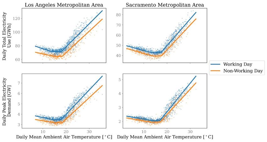
Environ. Res. Lett. 16 (2021) 074003                                                                                          Z Wang et al

   Figure 1. City-scale electricity use by different ambient air temperature: (a), (b), represents the impact of ambient air temperature
   on daily total electricity consumption for the Los Angeles Metropolitan Area (a) and the Sacramento Metropolitan Area (b)–(d),
   represents the impact of ambient air temperature on daily peak electricity demand for the Los Angeles Metropolitan Area (c) and
   Sacramento Metropolitan Area (d).

to heat exhaustion, heat edema, heat cramps, heat                           In figure 1, a clear pattern can be observed show-
syncope, and heatstroke [12], all of which are dan-                    ing that higher ambient temperature would drive up
gerous health risks and can cause a public health                      city-scale electricity consumption. We extracted the
crisis.                                                                elasticity of city-scale electricity use and peak demand
                                                                       on ambient daily mean temperature in table 1. Com-
                                                                       pared with the base load, 1 ◦ C increase of ambient
1.1. Heat wave and grid stress
                                                                       temperature drives up the daily total electricity con-
In modern society, the building sector accounts for
                                                                       sumption by 4.7% in the Los Angeles region and 6.2%
32% of global energy demand (24% for residen-
                                                                       in Sacramento; while it increases the daily peak elec-
tial and 8% for commercial) [13]. Among building
                                                                       tricity demand by 6.9% in the Los Angeles Metropol-
end users, heating, ventilation, and air-conditioning
                                                                       itan Area and 9.2% in Sacramento.
(HVAC) is a major electricity consumer, consum-
                                                                            The dramatic increase in electricity demand dur-
ing 33% of total building energy consumption in
                                                                       ing heat waves poses challenges to grid operation
Hong Kong [14], 40% in Europe [15], 50% in the
                                                                       and energy security. On August 14 and 15, 2020,
United States [16], and more than 70% in Middle
                                                                       Northern California residents experienced a rotat-
East countries [17]. During heat waves, people tend
                                                                       ing power outage event. The major factor that led
to stay inside air-conditioned environments for a
                                                                       to the rotating outages was that California experi-
longer period and extend their use of air condition-
                                                                       enced a one-in-thirty-year extreme heat wave in mid-
ing. In addition, the higher outdoor air temperature
                                                                       August of 2020 [20]. The heat wave drove up the
increases the cooling loads in buildings. These two
                                                                       electricity demand, which exceeded the existing elec-
factors combined lead to significant increases of elec-
                                                                       tricity resource planning targets. The California Inde-
tricity demand to cool buildings.
                                                                       pendent System Operator Corporation was forced to
     In figure 1, we applied a five-parameter change
                                                                       institute rotating power outages because the increas-
point model [18] to examine how ambient air tem-
                                                                       ing electricity demand could not be met by electri-
perature is correlated with city-scale electricity con-
                                                                       city generated locally or imported from neighbouring
sumption in two major metropolitan areas in Califor-
                                                                       areas, as this extreme weather event extended across
nia: Los Angeles and Sacramento. We used the hourly
                                                                       the Western United States and accordingly strained
data of two Californian Balancing Authorities—the
                                                                       the resources in neighbouring areas as well. As a res-
Los Angeles Department of Water & Power (LADWP)
                                                                       ult, rotating power outages were instituted.
and the Balancing Authority of Northern Califor-
nia (BANC)—collected by the U.S. Energy Inform-
ation Administration [19] between 2015 and 2020.                       1.2. Research gaps and objectives
LADWP and BANC recorded the electricity use in                         A rotating power outage exposes residents to over-
the Los Angeles and Sacramento Metropolitan Areas,                     heating risks due to the lack of air conditioning dur-
respectively.                                                          ing the extreme heat wave event. If a rotating power

                                                        2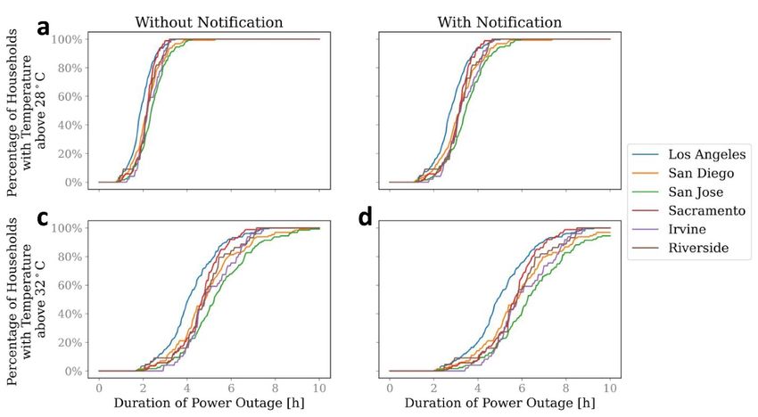
Environ. Res. Lett. 16 (2021) 074003                                                                                          Z Wang et al

              Table 1. Sensitivity of city-scale electricity use and peak demand to the daily mean ambient air temperature.

                                 Daily electricity use (MWh ◦ C−1 )                 Daily peak electricity demand (MW ◦ C−1 )
                                Working days               Non-working days             Working days             Non-working days

Los Angeles                            3.40                      3.15                        0.24                        0.21
Metropolitan Area
Sacramento                             2.62                      2.43                        0.20                        0.18
Metropolitan Area

outage is unavoidable, a key question in planning the                 and the contribution and limitation of this study in
power outage is how long it should last, so occupants’                section 4.2 before we conclude in section 5.
overheating risks can be minimized. The allowable
maximal power outage duration depends on both the
severity of the heat wave (i.e. how high the ambi-
                                                                      2. Method
ent temperature is and for how long it lasts) and
                                                                      We proposed a two-step approach to determine
the thermal property of the buildings. The conven-
                                                                      the maximum allowable power outage duration, as
tional way to investigate the building thermal per-
                                                                      shown in figure 2.
formance is through either a questionnaire survey or
                                                                          The first step is to infer thermal dynamics of resid-
on-site physical inspection. Two examples of those
                                                                      ential building stock. As discussed in the Background
efforts are the English Housing Survey (EHS) [21]
                                                                      section, the conventional approach to investigate
and the U.S. Residential Energy Consumption Sur-
                                                                      building thermal characteristics is constrained by its
vey [22]. However, those conventional approaches are
                                                                      high costs and small sample size. In this study, we
expensive and usually not adequately representative.
                                                                      proposed a data-driven hybrid (grey-box) modelling
For instance, the U.S. RECS is conducted every four to
                                                                      approach: using a thermal resistance-capacity net-
six years and limited to a small sample size (e.g. 5686
                                                                      work model (R-C model) to characterize the building
households throughout the country in the 2015 sur-
                                                                      thermal dynamics and then using the smart thermo-
vey [23]). Meanwhile, for many places of the world,
                                                                      stat data to estimate the value of the model’s paramet-
the information of building thermal property is not
                                                                      ers; in this case, the value of thermal resistance (R)
available, which makes rotating power outage plan-
                                                                      and thermal capacity (C) of a house. The dataset we
ning challenging.
                                                                      used in this study is Ecobee DYD Dataset [24]. The
    In this study, we propose a novel approach to
                                                                      sampling rate of this dataset is 5 min and the temper-
inform decision makers and grid operators when
                                                                      ature measurement resolution is 1 ◦ F.
planning the inevitable rotating power outages. This
approach was tested using the 2020 rotating power
outage in California, and has the potential to be                     2.1. Thermal dynamic reduced-order model
used in other places of the world. We first applied                   Inspired from the thermal-electrical analogy,
a novel data-driven inverse modelling method to                       researchers proposed the R-C heat transfer network
infer building thermal property using a state-wide                    model to simulate the thermal dynamics of a building
open source dataset collected from connected smart                    [25]. There are various orders of R-C models [26], i.e.
thermostats—the Ecobee Donate Your Data (DYD)                         different numbers of Rs and Cs in the R-C network.
program [24]. Then the inferred building thermal                      Similar to other machine learning algorithms, higher-
characteristics were used to plan the power outage                    order models can deliver a more accurate model pre-
by simulating the thermal resilience of the residential               diction but may suffer from over-fitting. Once the
building stock.                                                       model order is determined, the model parameters
    This study is organized as follows, we first intro-               (e.g. values of R and C) are estimated by fitting the
duce the novel hybrid inverse modelling approach                      measured data. In this study, we selected a 1R–1C
in section 2, where we describe the thermal dynam-                    model, as it could deliver a prediction with a root
ics model (section 2.1), the parameter estimation                     mean squared error (RMSE) of less than 0.5 ◦ C, while
method (section 2.2) and model validation approach                    avoiding over-fitting risks.
(section 2.3) in greater details. Then we present the                     The reduced order model used to simulate a
results and major findings in section 3: we com-                      residential building’s thermal dynamics is shown in
pare the identified thermal properties between differ-                equation (1), where Tin and Tout are the indoor
ent major cities in California (section 3.1), and then                and outdoor air temperature, R and C represent the
simulate the thermal resilience during a heat wave                    thermal resistance and thermal capacity of the build-
event using the identified parameters (section 3.2).                  ing, QHVAC represents the heat from HVAC (a negative
We will discuss the recommended power outage dura-                    value for cooling and a positive value for heating), and
tion that could avoid overheating risks in section 4.1,               Teq is the equivalent temperature rise that considers

                                                       3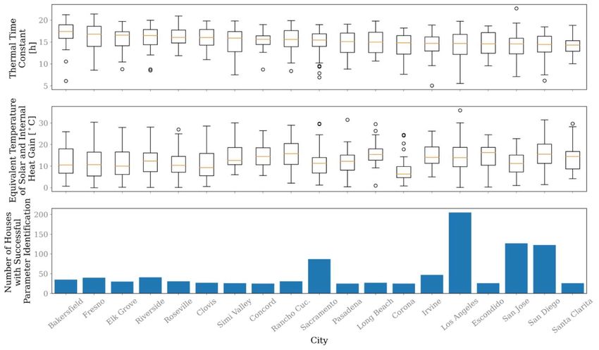
Environ. Res. Lett. 16 (2021) 074003                                                                                          Z Wang et al

   Figure 2. The data analytics process to inform the maximum power outage duration in California: We proposed this two-step
   approach to estimate the allowable maximum power outage duration in California. The first step is to infer the thermal
   characteristics of residential building stock in California using the connected smart thermostat data. The second step is to predict
   the thermal states when a power outage happens using the inferred thermal dynamics, and based on that prediction, to estimate
   the allowable maximum power outage duration.

solar irradiation and internal heat gains (from occu-                  two terms on the right hand side of equation (1) con-
pants, lights, and appliances use). The term Teq                       sistent and comparable. The value of Teq depends
characterizes the effect of solar and internal heat                    on (a) local solar condition, (b) some building char-
gains, which is defined as Teq = R∗ (Qsolar + Qinternal ).             acteristics that are not reflected by R, including the
The physical implication of Teq is: because of the                     building’s orientation, window-to-wall ratio, shad-
solar and internal heat gains, the outdoor tem-                        ing, and window performance. For instance, houses
perature Tout is equivalently increased by Teq . Teq                   with a large window-to-wall ratio and large win-
depends on the house’s characteristics: orientation,                   dow solar heat gain coefficient are exposed to larger
shading, window-to-wall ratio, and window thermal                      solar heat gains and therefore have a larger Teq . As
properties                                                             Teq varies building to building, it is inferred through
                                                                       the parameter estimation process as well. The third
          dTin    (Tout − Tin ) Teq                                    term represents the heating or cooling provided by
        C       =                +     + QHVAC .      (1)
           dt           R            R                                 HVAC.
As shown in equation (1), the indoor air temper-                            In the first-order, linear time-invariant (LTI) sys-
ature change is driven by three terms: heat trans-                     tem, the concept of time constant is widely used to
fer between indoor and outdoor (including heat                         characterize the system’s response to a step input.
exchange through exterior envelope and air filtra-                     Physically, the time constant represents the elapsed
tion), solar and internal heat gains, and heating or                   time required for the system’s response to a step
cooling provided by the HVAC. On the left hand side                    signal. In a dynamic system that the variable is
of equation (1), the thermal capacity term includes                    increasing, the time constant is the time the vari-
the thermal capacity of the envelope, furniture, and                   able reaches 63.2% of its final (asymptotic) value
indoor air. In terms of the first term on the right hand               in the step response. In a system that the variable
side, the thermal resistance term takes into account                   is decreasing, the time constant is the time it takes
not only the heat transfers through the building envel-                for the system’s step response to reach 36.8% of its
ope, but also the heat transfers through air infiltra-                 final value. Residential buildings’ thermal dynamics
tion. As for the second term on the right hand side,                   after the cooling is turned off during a power out-
the influence of solar radiation and internal heat gains               age event is like an LTI system’s step response [27].
is captured by adding an extra equivalent temper-                      Therefore, we used the thermal time constant (TTC)
ature term, Teq , to the ambient air temperature. It                   as a key parameter to evaluate the thermal resili-
is worthwhile to point out that Teq is normalized                      ence of residential buildings during a power outage
(by R) of Qsolar + Qinternal , which can make the first                event.

                                                        4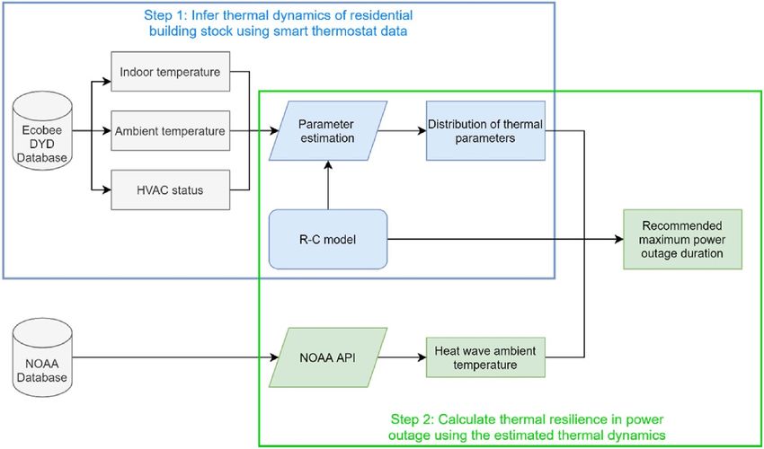
Environ. Res. Lett. 16 (2021) 074003                                                                                      Z Wang et al

                                       Table 2. Rules to select data for parameter identification.

                           Heating season                                                 Cooling season

QHVAC = 0                  Free floating period (heating is off)                          Free floating period (cooling is off)
Teq                        Data between 10 PM and 7 AM, Teq = 0                           Data between 10 AM and 3 PM; the first
                                                                                          three hours or less period of free floating,
                                                                                          Teq is constant
Fitting quality            Free floating period lasts at least 1.5 h                      Free floating period lasts at least 1.5 h
                           Temperature decrease is more than 2 ◦ C                        Temperature increase is more than 2 ◦ C
                           during this free floating period                               during this free floating period
                           RMSE is less than 0.5 ◦ C                                      RMSE is less than 0.5 ◦ C

2.2. Inferring thermal parameters                                     of our assumptions might be invalid, for instance,
In the thermal dynamic model of equation (1), there                   Teq did not stay constant for this household dur-
are three types of variables:                                         ing this period. We summarized the assumptions in
                                                                      table 2.
• Parameters to be estimated: R, C, Teq                                    Because of the data quality issue and the restric-
• Measured variables: Tout , Tin                                      tions we used to select the data, we could not infer
• Unmeasured variables: QHVAC                                         the thermal properties for every residential building
                                                                      recorded in the database. Figure 3 plots the three
    To facilitate the parameter identification, we pro-               major error types we encountered during the para-
posed some rules and applied them to select sev-                      meter identification process. The sample size of the
eral chunks of data that can be used for system                       database increased by more than eight times between
identification.                                                       2015 and 2019. The major reason the parameter iden-
                                                                      tification failed in heating season is that the tem-
• Since the Ecobee DYD dataset does not record                        perature variation during free floating was less than
  energy-related data, QHVAC is not available. As a                   2 ◦ C, because California generally has a mild winter.
  solution, we selected the time when heating or cool-                The major reason the parameter identification failed
  ing was turned off (a.k.a. the free-floating period)                in cooling season is that we could not find quali-
  to get rid of the term QHVAC in the model.                          fied free floating periods, for two reasons. First, cool-
• In the heating season, we used the data between                     ing is less frequently used in Californian households.
  10 PM and 7 AM for parameter inference, because                     Second, fewer residents turned off cooling during 10
  during this period (a) the solar heat gain was zero,                AM to 3 PM. On the contrary, more occupants tend
  (b) the internal heat gain was marginal, and (c) the                to turn off heating or reset to a lower indoor temper-
  outdoor air temperature was the lowest. Therefore,                  ature setpoint after they fall sleep, therefore it is more
  we can assume Teq is 0, and the term (ToutR−Tin ) rep-              likely to find a free-floating period during 10 PM and
  resents the right-hand side of equation (1) during                  7 AM. Once we were able to find a qualified data
  this period.                                                        fitting period, the model was able to deliver regres-
• In cooling season, Teq is not negligible. We used                   sions with few households having an RMSE larger
  the data around noon (between 10 AM and 3 PM)                       than 0.5 ◦ C.
  because we wanted to infer the largest Teq (due to
  the solar radiation), which is needed in the worst                  2.3. Model validation
  scenario analysis of thermal resilience. Addition-                  We applied two methods to validate our approach. We
  ally, we used less than three hours of data so we can               first validate our model with the real measurement
  (a) assume Teq was constant during the model fit-                   data. Figure 4 plots the measured and predicted tem-
  ting, and (b) identify the largest solar heat gain for              perature of a random winter and summer day, show-
  worst scenario analysis.                                            ing a good fitness of our model.
• We selected the free-floating periods that lasted                        The second validation approach is to the values
  more than 1.5 h and with a temperature change of                    of the thermal time constant of the same households
  more than 2 ◦ C because more data points and lar-                   inferred from heating and cooling seasons. Theor-
  ger state variations could help the system identific-               etically, TTC inferred from summer data and TTC
  ation process.                                                      inferred from winter data should be similar unless
                                                                      there is a major retrofit of the building. The box plot
     We used scipy.optimize [28] for parameter iden-                  of figure 5 shows a good consistence between the TTC
tification. Once the parameter fitting was done, we                   median values and ranges between the 25% and 75%
only kept those results with a RMSE less than 0.5 ◦ C.                percentiles. The variation of TTC inferred from the
We dropped those data points if the RMSE was lar-                     cooling season was larger than that inferred from the
ger than 0.5 ◦ C because a large RMSE indicates some                  heating season for two reasons. First, as shown in

                                                       5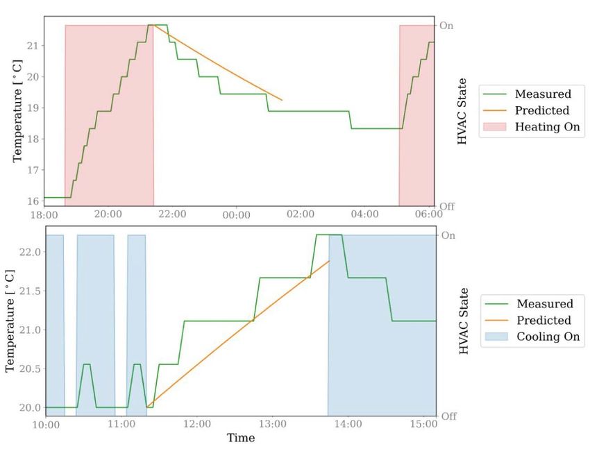
Environ. Res. Lett. 16 (2021) 074003                                                                                         Z Wang et al

   Figure 3. Error types encountered during the parameter identification process: panel (a) shows the heating season; panel
   (b) shows the cooling season.

   Figure 4. Parameter identification results for a typical winter and summer day: parameter identification results for a typical
   winter (panel (a)) and summer (panel (b)) day. The resolution of recorded temperature in the Ecobee DYD database is
   1 ◦ F (0.56 ◦ C), therefore the measured data demonstrate a discrete change behaviour.

                    Figure 5. Boxplot of thermal time constants derived from data recorded in winter and summer.

                                                        6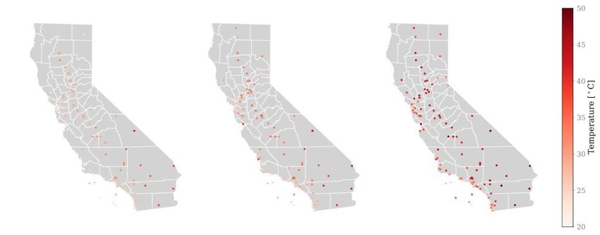
Environ. Res. Lett. 16 (2021) 074003                                                                                        Z Wang et al

   Figure 6. Regressed parameters for major Californian cities: The regressed key parameters of Californian cities with the largest
   sample size in the Ecobee DYD database. Panel (a) is the boxplot of regressed thermal time constant. Panel (b) is the boxplot of
   regressed equivalent temperature of solar and internal heat gains. Panel (c) is the number of residential buildings with thermal
   properties successfully identified. The cities are ordered by the median value of the thermal time constant.

figure 3, the sample size of residential buildings with               heat gains drive up the Teq of residential buildings in
successful parameter identification was larger in the                 Southern California.
heating season. Second, the temperature difference
between indoor and outdoor temperature in heating
season was larger, therefore the indoor temperature                   3.2. Thermal resilience in power outage
variation was larger during free-floating mode in the                 After the thermal dynamics are identified, we apply
heating season. A larger temperature variation facilit-               them to simulate the indoor thermal states when a
ates a more accurate parameter identification.                        power outage happens. As air conditioning is turned
                                                                      off during a power outage, the building enters the
                                                                      ‘free-floating’ mode. The rates of indoor temperature
3. Result                                                             increase depend on the ambient weather conditions
                                                                      and the building thermal properties: a higher ambi-
3.1. Thermal properties of Californian residential                    ent temperature, higher Teq , and smaller TTC lead to
buildings                                                             a faster temperature increase. In this study, we con-
We plotted the distribution of estimated TTC and                      sidered the worst scenario by using the highest hourly
Teq for Californian cities that have more than 25 suc-                temperature of 2020 as the ambient air temperature
cessful parameter identification houses in figure 6.                  of each city and inferring the Teq of the noon time
It could be observed that cities in the Central Val-                  (see the Method section). The impact of solar radi-
ley (Fresno, Bakersfield, and Clovis) and Northern                    ation is considered by using Teq inferred from his-
California (Sacramento) have larger TTC values com-                   torical data, assuming the contribution of solar heat
pared with cities in the Southern Coast region (Los                   gains stay about the same during the heat wave event.
Angeles, Santa Clarita, Irvine). This is partly because                   We used the API provided by the National
the California Building Energy Efficiency Standards                   Oceanic and Atmospheric Administration (NOAA)
[29] require building thermal insulation in colder cli-               [30] to download the weather data. We downloaded
mate zones to be higher. Better building thermal insu-                the weather data from the geographically closest
lation leads to a larger thermal time constant.                       weather station for each city during 2020. To con-
    In terms of Teq , Southern California cities such as              sider the worst scenario, we used the hourly max-
Los Angeles, San Diego, and Rancho Cucamonga have                     imum temperature as the inputs to analyse the resid-
larger Teq than Northern California cities (e.g. Sacra-               ential buildings’ thermal resilience during the power
mento, San Jose). This is because Southern Califor-                   outage. The hourly maximum ambient temperature
nia cities have more sunshine, leading to higher solar                during the heat wave reached 50 ◦ C in some regions,
heat gains for residential buildings. The higher solar                as shown in figure 7.

                                                       7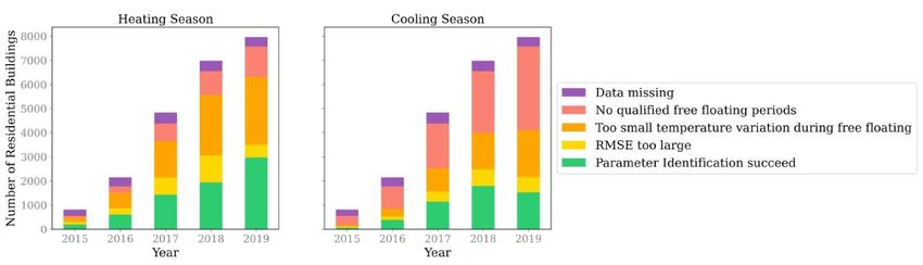
Environ. Res. Lett. 16 (2021) 074003                                                                                 Z Wang et al

   Figure 7. Weekly, daily, and hourly maximum ambient air temperature in 2020 measured by NOAA weather stations in
   California: The locations of National Oceanic and Atmospheric Administration (NOAA) weather stations and the recorded
   weekly (panel (a)), daily (panel (b)), and hourly (panel (c)) peak ambient temperature in 2020.

    To determine the allowable maximum power out-                 by a higher Teq in figure 6(b)), and (c) houses in
age duration, we needed a clear definition of over-               Los Angeles have less insulation (reflected by a smal-
heating risks in residential buildings. Based on the              ler uate the the TTC in figure 6(a)). The pre-cooling
heat index classification of NOAA, the occupants                  measure can increase the allowable maximum power
should be Cautious when the indoor heat index is                  outage duration by about an hour in both cases.
above 80 ◦ F (26.7 ◦ C) and Extremely Cautious when                   Figure 9 shows a plot of the percentage of house-
the indoor heat index is above 90 ◦ F (32.2 ◦ C)                  holds exposed to overheating risks as a function of
[31]. In Europe, based on the Chartered Institu-                  power outage duration for four Californian cities: Los
tion of Building Services Engineers’ Environmental                Angeles (largest California city by population), San
Design Guideline, there should be no more than 1%                 Diego (2nd), San Jose (3rd), Sacramento (6th), Irvine
of annual occupied hours over an operative temper-                (14th), and Riverside (12th). Those six cities have
ature of 28 ◦ C in living rooms, and no more than                 the largest sample sizes in the Ecobee DYD database.
1% of annual occupied hours over an operative tem-                A higher percentage of households are exposed to
perature of 26 ◦ C in bedrooms [32]. In this study                overheating risks with increasing power outage dur-
we used 28 ◦ C and 32 ◦ C as the two thresholds of                ation. Because the indoor temperatures of houses in
overheating.                                                      Los Angeles increase the fastest, the highest percent-
    We considered two scenarios: (a) not notifying                age of households are exposed to overheating risks
residents about the power outage and (b) notifying                in Los Angeles given the same power outage dura-
residents about the power outage in advance; corres-              tion. Conversely, households in San Jose, a Northern
ponding to the two initial conditions. When the res-              Californian city, have the lowest overheating risk dur-
idents have not been notified about the power outage,             ing the power outage event.
we assumed the initial condition to be an indoor tem-
perature of 24 ◦ C. If the residents have been notified           4. Discussion
about the power outage in advance, they might take
some pre-cooling measures to further cool down the                4.1. Recommended power outage duration
indoor environment before the power outage, there-                The determination of power outage duration to avoid
fore the initial condition of indoor temperature was              overheating risks of residents depends on two criteria:
assumed to be 22 ◦ C (which is at the lower end of                (a) the acceptable maximum indoor air temperature,
ASHRAE cooling temperature range from 22 ◦ C to                   (b) the allowable percentage of households exposed
25 ◦ C) once the cooling was shut off.                            to overheating risk. In this study, the recommended
    The evolution of indoor temperature during a                  allowable power outage duration was determined as
power outage event is plotted in figure 8. We plot-               the maximum period that less than 10% of house-
ted Los Angeles and San Jose because these two cities             holds are exposed to overheating risks. We selected
had the largest sample size in the database and also              28 ◦ C as the threshold value because we wanted to
are among the biggest cities by population in Califor-            be more conservative. In extreme scenarios to avoid
nia. The temperatures of San Jose’s houses rise slower            power blackout of the entire power grid, a higher tem-
than those of Los Angeles’s houses for three reasons:             perature such as 30 ◦ C or even 32 ◦ C may be con-
(a) Los Angeles has a higher ambient temperature,                 sidered. We chose 90% rather than 100% of house-
(b) Los Angeles has higher solar heat gains (reflected            holds to be free of overheating for two reasons: (a) to

                                                    8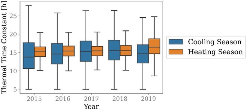
Environ. Res. Lett. 16 (2021) 074003 Z Wang et al
Figure 8. Evolution of indoor air temperature during a power outage: The evolution of indoor air temperature during a power
outage event: (a), (b) for residential buildings in Los Angeles; (c), (d) for residential buildings in San Jose; (e), (f) for how long
the indoor temperature takes to raise to 28 ◦ C during a power outage; (a), (c), (e) for without notification (no pre-cooling);
(b), (d), (f) for with notification (pre-cooling). Each line in a–d represents a household. The two horizontal lines represent the
28 ◦ C and 32 ◦ C overheating risk thresholds, respectively.
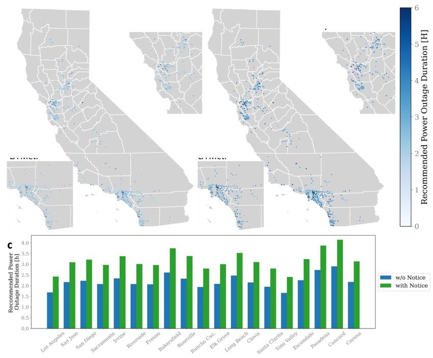
Figure 9. Percentage of households exposed to overheating risks during a power outage: the percentage of households exposed to
overheating risks as a function of power outage duration in six Californian cities: panel ((a), (c)) for Scenario a shows households
not notified about power outage events in advance, panel ((b), (d)) for Scenario b shows households notified about power outage
events in advance and, accordingly, taking some pre-cooling measures; panel ((a), (b)) shows an overheating threshold of 28 ◦ C;
panel ((c), (d)) shows an overheating threshold of 32 ◦ C.
9Environ. Res. Lett. 16 (2021) 074003 Z Wang et al
Figure 10. Recommended allowable power outage duration to avoid overheating risks: Recommended allowable power outage
duration for Californian cities: without advance notification (panel (a)), with advance notification (panel (b)), and for cities with
sample sizes larger than 25 (panel (c)). The dot size of panel (a), (b) represents the sample size of the city.
account for measurement uncertainty and modelling thermostat data of 85 thousand U.S. households.
error, and (b) to avoid the results dominated by the In California, we have 8399 samples out of 11 500
few poorly insulated houses. The criteria to determine thousand households state-wide, and the sample rate
the maximum allowable power outage duration can is 0.70 samples per thousand households, exceed-
be set by the local grid operators. We plotted the ing the sample rate of RECS by 23 times. Third, the
recommended power outage duration for Californian hybrid grey-box approach integrates the strengths of
cities in figure 10. Informing the residents in advance a data-driven, physics-based model: achieving a high
of a power outage, so they can cool down their houses modelling accuracy with clear physical implications.
to a lower temperature before the power outage, is a The developed R-C models and inferred parameters
simple and effective strategy to increase the acceptable can be used for other applications, such as to estim-
power outage duration—by more than one hour for ate the load shifting potential of residential building
most cities. stocks by leveraging the passive thermal storage of
building structures, and to evaluate building thermal
4.2. Contribution and limitation efficiency policies.
The advantages of our proposed approach are The major limitation of this approach lies in
threefold. First, it can save costs and labour com- the potential sample bias. We can only sample from
pared with conventional methods of investigating households that have installed the smart thermostats,
the thermal properties of building stock, because which may not be a random sampling from the whole
we are using the existing Ecobee DYD database. population. Even though some researchers found that
Second, the sample size of this method is larger the technology adoption intention is not influenced
than the existing data sources, which enables a more by household income [33], there is a lack of evid-
robust, accurate, and reliable estimation of a build- ence to support the idea that the residential buildings
ing’s thermal performance. For instance, the RECS recorded in the Ecobee DYD database are a random
surveyed 5.6 thousand households once every four sampling of the whole residential stock. The posit-
years. The Ecobee DYD database recorded the smart ive side is, with the penetration of smart thermostat
10Environ. Res. Lett. 16 (2021) 074003 Z Wang et al
technology and increasing number of households that during heat waves to avoid overheating risks. Inform-
are willing to donate their data (the sample size of the ing the residents in advance, so they can cool down
DYD dataset increased from 7000 in 2015 to 101 000 their houses to a lower temperature before power
in 2019), this method could gradually approach the outages during heat waves, is a simple and effective
true thermal property distribution of the residential strategy to increase the acceptable power outage dur-
building stock. ation by about one hour.
Another limitation of the approach is the use of
the one order R-C model and the related assump- Data availability statement
tions, which may lead to larger errors for certain indi-
vidual houses. However, our study focus on the build- The data that support the findings of this study are
ing stock level. Quite some households’ data cannot available upon reasonable request from the authors.
be used in the study due to the modelling assumptions
and selection process. However, with the continu-
ous growth of data in the Ecobee DYD dataset, many Acknowledgments
more valid households’ data can be used in future
This research was supported by the Assistant Sec-
research.
retary for Energy Efficiency and Renewable Energy,
Office of Building Technologies of the United
5. Conclusion
States Department of Energy, under Contract No.
DE-AC02-05CH11231. Authors thank Ecobee and
With climate change, heat waves become more fre-
their customers for making the DYD dataset available
quent and intense. Heat waves pose new challenges
for research.
to energy security and public health as they drive up
electricity demand and expose residents to overheat-
ing risks. In extreme cases, when the power supply is
unable to meet the demand increase, rotating power ORCID iD
outages are instituted. Californian residents experi-
enced rotating power outages in August 2020, when a Tianzhen Hong https://orcid.org/0000-0003-
historic heat wave extended across the western United 1886-9137
States. The lack of space cooling during a power
outage during heat waves exposes residents to high References
overheating risks, which could cause a public health
crisis. [1] Robinson P J 2001 On the definition of a heat wave J. Appl.
Meteorol. Climatol. 40 762–75
If a power outage is unavoidable during heat
[2] Smoyer-Tomic K E, Kuhn R and Hudson A 2003 Heat wave
waves, it is essential to understand how long the hazards: an overview of heat wave impacts in Canada Nat.
power outage can last, so the grid stress can be relieved Hazards 28 465–86
while minimizing occupants’ overheating risks. In [3] Meehl G A and Tebaldi C 2004 More intense, more frequent,
and longer lasting heat waves in the 21st century Science
this study, we proposed a data-driven inverse mod-
305 994–7
elling approach to inform decision makers and grid [4] Van Oldenborgh G J, Philip S, Kew S, Van Weele M, Uhe P,
operators on planning a rotating power outage. Our Otto F, Singh R, Pai I, Cullen H and AchutaRao K 2018
proposed approach was tested using data from the Extreme heat in India and anthropogenic climate change
Nat. Hazard Earth Syst. Sci. 18 365–81
California rolling power outage in August 2020.
[5] Trenberth K E and Fasullo J T 2012 Climate extremes and
Our method includes two steps: (a) infer the climate change: the Russian heat wave and other climate
thermal characteristics of residential building stock extremes of 2010 J. Geophys. Res. Atmos.
using the connected smart thermostat data, and (b) 117 D17103
[6] Xia J, Tu K, Yan Z and Qi Y 2016 The super-heat wave in
simulate the thermal states when a power outage hap-
eastern China during July–August 2013: a perspective of
pens using the inferred thermal dynamics, based on climate change Int. J. Climatol. 36 1291–8
the prediction to recommend the maximum allow- [7] Robine J-M, Cheung S L K, Le Roy S, Van Oyen H,
able power outage duration. Griffiths C, Michel J-P and Herrmann F R 2008 Death toll
exceeded 70 000 in Europe during the summer of 2003 C. R.
We tested our approach in California, with spe-
Biol. 331 171–8
cial focus on large Californian cities with large [8] Hoag H 2014 Russian summer tops ‘universal’ heatwave
sample sizes. We first inferred the thermal prop- index Nat. News D16250
erties of residential stock using the Ecobee DYD [9] Guo Y et al 2018 Quantifying excess deaths related to
heatwaves under climate change scenarios: a multi-
dataset. Residential buildings in Northern Califor-
country time series modelling study PLoS Med.
nia cities have a larger thermal time constant due to 15 e1002629
more stringent building thermal regulations. Then we [10] Sathaye J A, Dale L L, Larsen P H, Fitts G A, Koy K,
applied the inferred models to simulate the thermal Lewis S M and De Lucena A F P 2013 Estimating impacts of
warming temperatures on California’s electricity system
resilience of residential buildings during the power
Glob. Environ. Change 23 499–511
outage. For the majority of Californian cities, the [11] Zhao L et al 2021 Global multi-model projections of local
power outage should not last more than two hours urban climates Nat. Clim. Change 11 152–57
11Environ. Res. Lett. 16 (2021) 074003 Z Wang et al
[12] Bouchama A and Knochel J P 2002 Heat stroke New Engl. J. [23] U.S. Energy Information Administration RECS: comparing
Med. 346 1978–88 the 2015 RECS with previous RECS and other studies
[13] Ürge-Vorsatz D, Cabeza L F, Serrano S, Barreneche C and (available at: www.eia.gov/consumption/residential/reports/
Petrichenko K 2015 Heating and cooling energy trends and 2015/comparison/) (Accessed 12 January 2021)
drivers in buildings Renew. Sustain. Energy Rev. 41 85–98 [24] Ecobee Donate your data smart Wi-Fi thermostats (available
[14] Fong K F, Chow T T, Lee C K, Lin Z and Chan L S 2010 at: www.ecobee.com/donate-your-data/) (Accessed 12
Comparative study of different solar cooling systems for January 2021)
buildings in subtropical city Sol. Energy 84 227–44 [25] Fraisse G, Virgone J and Menezo C 2000 Proposal for a
[15] Balaras C A et al 2007 Solar air conditioning in Europe—an highly intermittent heating law for discontinuously occupied
overview Renew. Sustain. Energy Rev 11 299–314 buildings Proc. Inst. Mech. Eng. Part J. Power Energy
[16] Pérez-Lombard L, Ortiz J and Pout C 2008 A review on 214 29–39
buildings energy consumption information Energy Build. [26] Wang Z, Luo M, Geng Y, Lin B and Zhu Y 2018
40 394–8 A model to compare convective and radiant heating systems
[17] El-Dessouky H, Ettouney H and Al-Zeefari A 2004 for intermittent space heating Appl. Energy 215 211–26
Performance analysis of two-stage evaporative coolers Chem. [27] Wang Z, Lin B and Zhu Y 2015 Modeling and measurement
Eng. J. 102 255–66 study on an intermittent heating system of a residence in
[18] Kissock J K, Haberl J S and Claridge D E 2002 Development Cambridgeshire Build. Environ. 92 380–6
of a toolkit for calculating linear, change-point linear and [28] The SciPy community Optimization and root finding
multiple-linear inverse building energy analysis models, (scipy.optimize)—SciPy v1.6.0 reference guide (available at:
ASHRAE research project 1050-RP, Final Report Energy https://docs.scipy.org/doc/scipy/reference/optimize.html)
Systems Laboratory, Texas A&M University, Technical (Accessed 19 January 2021)
Report Nov (available at: https://oaktrust.library.tamu. [29] California Energy Commission 2016 Building energy
edu/handle/1969.1/2847) (Accessed 19 January efficiency standards for residential and nonresidential
2021) buildings
[19] Ruggles T H, Farnham D J, Tong D and Caldeira K 2020 [30] National Climatic Data Center Web services API (version 2)
Developing reliable hourly electricity demand data through documentation Climate Data Online (CDO) (available at:
screening and imputation Sci. Data 7 1 www.ncdc.noaa.gov/cdo-web/webservices/
[20] California Independent System Operator Final root cause v2#gettingStarted) (Accessed 14 January 2021)
analysis: mid-August 2020 extreme heat wave (available at: [31] N. US Department of Commerce 2021 What is the heat
www.caiso.com/Documents/Final-Root-Cause-Analysis- index? (available at: www.weather.gov/ama/heatindex)
Mid-August-2020-Extreme-Heat-Wave.pdf) (Accessed 14 January)
[21] U.K. Ministry of Housing, Communities & Local [32] Chartered Institution of Building Services Engineers 2015
Government English Housing Survey GOV.UK (available at: Guide A Environmental Design 8th edn (London: Chartered
www.gov.uk/government/collections/english-housing- Institution of Building Services Engineers)
survey) (Accessed 12 January 2021) [33] Chen B and Sintov N 2016 Bridging the gap between
[22] U.S. Energy Information Administration Residential energy sustainable technology adoption and protecting natural
consumption survey (RECS)—energy information resources: predicting intentions to adopt energy
administration (available at: www.eia.gov/consumption/ management technologies in California Energy Res. Soc. Sci.
residential/) (Accessed 12 January 2021) 22 210–23
12You can also read