Starship Sails Propelled by Cost-Optimized Directed Energy
←
→
Page content transcription
If your browser does not render page correctly, please read the page content below
Starship Sails Propelled by Cost-Optimized Directed
                               Energy

                                        James Benford

                                     Microwave Sciences

                   1041 Los Arabis Lane, Lafayette, CA 94549 USA

                                   jbenford@earthlink.net
Microwave and laser-propelled sails are a new class of spacecraft using photon acceleration. It is
the only method of interstellar flight that has no physics issues. Laboratory demonstrations of
basic features of beam-driven propulsion, flight, stability (‘beam-riding’), and induced spin, have
been completed in the last decade, primarily in the microwave. It offers much lower cost probes
after a substantial investment in the launcher. Engineering issues are being addressed by other
applications: fusion (microwave, millimeter and laser sources) and astronomy (large aperture
antennas). There are many candidate sail materials: carbon nanotubes and microtrusses,
beryllium, graphene, etc. For acceleration of a sail, what is the cost-optimum high power
system? Here the cost is used to constrain design parameters to estimate system power, aperture
and elements of capital and operating cost. From general relations for cost-optimal transmitter
aperture and power, system cost scales with kinetic energy and inversely with sail diameter and
frequency. So optimal sails will be larger, lower in mass and driven by higher frequency beams.
Estimated costs include economies of scale. We present several starship point concepts.
Systems based on microwave, millimeter wave and laser technologies are of equal cost at today’s
costs. The frequency advantage of lasers is cancelled by the high cost of both the laser and the
radiating optic. Cost of interstellar sailships is very high, driven by current costs for radiation
source, antennas and especially electrical power. The high speeds necessary for fast interstellar
missions make the operating cost exceed the capital cost. Such sailcraft will not be flown until
the cost of electrical power in space is reduced orders of magnitude below current levels.

Keywords: Starship, Interstellar Precursor, Directed Energy, Sail, Starwisp, Microwave, Laser,
Propulsion

Laser and microwave propelled sails are a new class of spacecraft that uses photon acceleration.
These sailships are the only method of interstellar flight that has no physics issues. Indeed,
laboratory demonstrations of basic features of beam-driven propulsion have been completed in
the last decade (primarily in the microwave). It offers much lower cost probes after a substantial
investment in the launcher. But how practical are its scale and economics? This cost question


                                              1
has not been treated. So there is no understanding of what a lower-cost system would look like.
nor have the variety of missions the beam-propelled sail method can embrace been explored
from a cost point of view: Almost all studies deal with interstellar probes, the hardest of
missions, but the far easier interplanetary missions have been little treated, even though they will
come first. Only cost analysis can give concrete ideas of how to take the first steps in this new
technology.
The cost is largely not the spacecraft, but the reusable launcher or ‘beamer’ (a system comprised
of beam source and antenna(s) to radiate it). I derive general relations for cost-optimal
transmitter aperture and beam power, then estimate both capital coat and operating cost of cost-
transmitters using current cost parameters ($/W, $/m2). Costs for large-scale manufacture of
transmitters and antennas are well documented. (However, costs for space manufacture not
known.) Below we account for economies of scale, which will be important, and characterize
specific missions. In particular,
        •       Interstellar probes for exploration of the Oort Cloud, characterization of the nearby
                interstellar medium, and its interaction with the Heliosphere.
        •       Starships, either as primary propulsion of the mothership or as a means of decelerating
                probes from the mothership for Exoplanet exploration as the mothership flies on.

1. Why Minimize Costs?

Why consider economics at this early stage? Cost matters because it makes a big constraint, a
game-changing difference. That’s how we decide on competing claims for resources. Other
starship propulsion methods, are typically nuclear: fission, fusion, their hybrid, and matter/anti-
matter. Their costs are unquantifiable, although we can be sure each ship will be very expensive.
We ask: for a given kinetic in the launched sail, what is the cost-minimum beaming system? The
usual method of cost optimization is to examine many alternative approaches to building a
system, estimating the cost of each, and then comparing them. This is a ‘bottom-up’ approach.
We offer a more general ‘top-down’ method based on analysis and actual experiences of
designers. This gives a broader approach, capable of embracing new mission ideas as they arise.
The cost of first steps in this field will be essential in planning how to proceed.
       Cost of beaming systems is driven by two elements
            •    Capital cost CC, divided into the cost of building the microwave source and the cost of
                 building the radiating aperture CA, and the
            •    Operating cost CO, meaning the operational labor cost and the cost of the electricity to
                 drive the system:

                                                 C = CC + CO
                                                                                                      (1)
                                                 CC = C A + CS

Note that we’ll find that, for high velocity missions, sails will have much smaller costs than the
system that accelerates them. Consequently,
                                  €            sail cost is not included in the capital cost.


                                                     2
To optimize, meaning minimize, the cost, the simplest approach is to assume power-law scaling
dependence on the peak power and antenna area. Using this cost-minimization approach, we
have been able to correctly estimate (to within 15%) the actual cost of ORION, a transportable,
self-contained HPM test facility first fielded in 1995 and currently in operation [1]
Examples of how cost optimization can make a big difference appear in Appendix A.


2 State of Knowledge

Microwave and Laser propelled sails are a new class of spacecraft that promises to revolutionize
future space travel. (For a general introduction to solar and beam-propelled sails, the reader is
referred to McInnes [2].)
2.1 Theory

The beam (microwave and laser)-driven sail spacecraft was first proposed by Robert Forward
[3,4]. The sail acceleration aS from photon momentum produced by a power P on a thin sail of
mass m and area A is


                                          aS = [η+1] P/σAc                                   (2)

where
   η is the reflectivity of the film of absorbtivity α,
   c the speed of light, σ the area mass
density,
   m=
   σ A,
  with
   A the sail area. . Note that we’ve neglected the payload mass by counting
only the sail. This may not be true for smaller sails such as the interstellar precursor discussed in
section 4.
The force from photon acceleration is weak, but is observed in the trajectory changes in
interplanetary spacecraft, because the solar photons act on the craft for years. For solar photons,
with power density ~1 kW/m2 at Earth’s orbit, current solar sail construction gives accelerations
~1 mm/s2, a very low acceleration. Shortening mission time means using much higher power
densities. In this case, to accelerate at one earth gravity requires ~10 MW/m2. However, for
launch from orbit into interplanetary and interstellar space, much lower accelerations, and hence
much lower power densities are needed.
Of the power incident on the sail, a fraction αP will be absorbed. In steady state, this must be
radiated away from both sides of the film, with an average temperature T, by the Stefan-
Boltzmann law
                                            αP=2A ε κ T4                                         (3)

where κ is the Stefan-Boltzmann constant and ε is emissivity. Eliminating P and A, the sail
acceleration is
                               aS = 2 κ/c [ε (η+1) /α] (T4/m)                           (4)


                                                    3
where we have grouped constants and material radiative properties separately. Clearly, the
acceleration is strongly temperature-limited, ~T4. This fact means that materials with low melt
temperatures (Al, Be, Nb, etc.) cannot be used for fast beam-driven missions. For example,
aluminum has a limiting acceleration of 0.36 m/s2,
  which
  is
  1 gee to lift off.)

Fig. 1. Carbon sail lifting off of rectangular waveguide under 10 kW microwave power at 2 gees
(four frames, first at top) in vacuum chamber [5]. Sail heats up, lifts off, and in the bottom frame
                                       the sail has flown away.
Will sails riding beams be stable? The requirement of beam-riding, stable flight of a sail
propelled by a beam, places considerable demands on the sail shape. Even for a steady beam, the
sail can wander off if its shape becomes deformed or if it does not have enough spin to keep its


                                                       4
angular momentum aligned with the beam direction in the face of perturbations. Beam pressure
will keep a concave shape sail in tension, and it will resist sidewise motion if the beam moves
off-center, as a sidewise restoring force restores it to its position [6]. Experiments have verified
that beam-riding does occur [7]. Positive feedback stabilization seems effective when the
sidewise gradient scale of the beam is the same as the sail concave slope. A broad conical sail
shape appears to work best.
The beam can also carry angular momentum and communicate it to a sail to help control it in
flight. Circularly polarized electromagnetic fields carry both energy and angular momentum,
which acts to produce a torque through an effective moment arm of a wavelength, so longer
wavelengths are more efficient in producing spin. This effect can be used to stabilize the sail
against the drift and yaw, which can cause loss of beam-riding, and allows ‘hands-off’ control of
the sail spin, and hence stability, at a distance.


2.3 Missions

It’s important to realize that for large-scale space power beaming to become a reality it must be
broadly attractive. This means that it must provide for a real need, make business sense, attract
investment, be environmentally benign, be economically attractive and have major energy or
aerospace firms support and lobby for it. Therefore, we include missions that could lead to
Starwisp missions, from an infrastructure base developed for smaller-scale missions.
Interplanetary Launch An early mission for microwave space propulsion is dramatically
shortening the time needed for solar sails to escape Earth orbit. By sunlight alone, sails take
about a year to climb out of the earth’s gravity well. Computations show that a ground-based or
orbiting transmitter can impart energy to a sail if they have resonant paths – that is, the beamer
and sail come near each other (either with the sail overhead an Earth-based transmitter or the sail
nearby orbits in space) after a certain number of orbital periods. For resonance to occur
relatively quickly, specific energies must be given to the sail at each boost. If the sail is coated
with a substance that sublimes under irradiation, much higher momentum transfers are possible,
leading to further reductions in sail escape time. This new method, already shown in the
laboratory, promises to greatly improve times to lift sails into interplanetary orbits. Simulations
of sail trajectories and escape time are shown in Fig. 2. In general, resonance methods can
reduce escape times from Earth orbit by over two orders of magnitude versus using sunlight
alone on the sail [8].


                                                5
Fig. 2 Beam-driven sail trajectory out of earth orbit. a) Simulation: time of beam
       acceleration is the thicker line. 2 b) Radius normalized to earth radius vs. time for sail [8].

While microwave transmitters have the advantage that they have been under development much
longer than lasers and are currently much more efficient and inexpensive to build, they have the
disadvantage of requiring much larger apertures for the same focusing distance. This is a
significant disadvantage in missions that require long acceleration times with correspondingly
high velocities. However, it can be compensated for with higher acceleration. The ability to
operate carbon sails at high temperature enables much higher acceleration, producing large
velocities in short distances, thus reducing aperture size. Very low-mass probes could be


                                                 6
launched from Earth-based microwave transmitters with maximum acceleration achieved over a few hours using apertures only a few hundred meters across. A number of such missions have been quantified. These missions are for high velocity mapping of the outer solar system, Jupiter, Kuiper Belt, Plutinos, Pluto and the Heliopause, and the interstellar medium. Meyer and co-workers [9] described an attractive interplanetary mission: rapid delivery of critical payloads within the solar system. For example, such emergencies as crucial equipment failures and disease outbreaks, can make fast delivery of small mass payloads to, say, Mars colonies, urgent. They describe missions with 175 km/sec speeds driven by lasers or microwaves at fast boost for a few hours of acceleration, coast at high speed, decelerate for a few hours into Mars orbit (by aerocapture or a decelerating beamer) -- transit time 10 days. The Benfords’ Mars Fast Track then extended this to missions with 5 gee acceleration near Earth. Using a ground station, acceleration occurs for a couple of hours for a 100 kg payload. Jordin Kare quantified a Jupiter mission with beamed energy [10]. Interstellar Probes are solar/interstellar boundary missions out to ~1000 AU. The penultimate is the interstellar precursor mission. For this mission class, operating at high acceleration the sail size can be reduced to less than 100 m and accelerating power ~100 MW focused on the sail [11]. At 1GW, sail size extends to 200 m and super-light probes reach velocities of 250 km/s for very fast missions. In a NIAC study, McNutt and co-workers have described such missions driven by rocket and gravity assists. Beaming power could make for shorter mission durations. Here transit time is a serious factor driving mission cost. Starships Truly the biggest and grandest mission. This concept requires very large transmitter antenna/lens and receiver (sail) optics (e.g., 1,000-‐km diameters for missions to 40 ly). A Space Solar Power station radiates a microwave beam to a perforated sail made of carbon nanotubes with lattice scale less than the microwave wavelength. The scale of the first concept was enormous, but Geoff Landis found ways to reduce it dramatically [12-‐15]. Systems much smaller than those of Forward were described by Frisbee [16], with peak power ~10 GW and size (~1km sail, ~1000 km antenna array aperture). Presumably, cost is also lowered, but has not been quantified. We describe here an economic approach to sailships for further reduction in power, size and cost. 3 Cost-Optimization of Beam-Driven Sails 3.1 Capital Cost Whatever the mission, to optimize sailships, meaning to minimize the cost, the simplest approach is to assume power-law scaling dependence on the peak power P and antenna area A. This is a well-established method in industry [17]. The basic equation follows from linear scaling with coefficients describing the dependence of cost on area and radiated electromagnetic power. Antenna (or optic, in the case of lasers) areal cost coefficient a($/m2) includes cost of the antenna, its supports and sub-systems for pointing and tracking and phase control, and is not to be confused with the sail acceleration aS. Radiated power cost coefficient p ($/W) includes the source, power supply, cooling equipment and prime power cost. 7
C A = aA
                                                 C S = pP                                         (5)
                                           C C = aA + pP

I neglect any fixed costs, which would vanish when we differentiate to find the cost optimum.
Mass production can decrease the€ cost of antenna elements and power modules, and will later be
included in ‘learning curve’ factors in the coefficients a and p. We assign from mission
requirements the beam frequency, final velocity, sail mass and diameter as an input parameter
with respect to optimization.
3.2 Capital Cost-Optimum Scaling
I formulate the cost equation using equation A4 (in Appendix B) in terms of P, then substitute for
R0. Note that V0 is the speed at R0, the point where beam size exceeds sail size and the beam is
switched off. This final speed, which when

                                             2                  2
                                       V0 mc       2.44V0 mc2
                                   P=            =                                                (6)
                                      R 0 [η + 1] 2D t Ds f[η + 1]

                                                           2   2    2

                         € C = aA + pP = aπD t + p 2.44V0 mc                                      (7)
                            C
                                           4      2D t Ds f[η + 1]

Collect constants into g:
                €
                                          aπD t 2     V 2mc 2                                     (8)
                                   CC =           + gp 0
                                            4          Dt Dsf

where

                            €            2.44     1.22
                                   g=           =      ≅ 0.65                                     (9)
                                        2[η + 1] η + 1
for reflectivity slightly
2
∂C C aπ pmV0 c2
= Dt − g 2
=0 (10)
∂D t 2 D t Ds f
⎡ 2g p mV0 2c 2 ⎤1/ 3
€ Dt opt
= ⎢ ⎥ (11)
⎣ π a Dsf ⎦
After some algebra,
€
2/3
4 5 2 / 3 1/ 3 ⎡ mV0 ⎤
2
c4/ 3
C opt
=
3 2
(p a )⎢⎢ D f ⎥⎥ (η + 1)2 / 3 (12)
⎣ s ⎦
opt opt
CP = CA
Minimum capital cost is achieved when the cost is equally divided between antenna gain and
radiated power. This derived result was used as a rule-of-thumb by microwave system designers
for rough estimates of system cost. This cost ratio was independently discovered from cost data
€
on the Deep Space Network [18]. For a recent example, Kare and Parkin have built a detailed
cost model for a microwave beaming system for a beam-driven thermal rocket and compared it
to a laser-driven rocket. They also find that, at minimum, cost is equally divided between the
two cost elements [19]. However, the power beaming relation in reference 17 for Copt
is
different
from
Eq.
12.
That’s
because
here
we
add
the
sails
acceleration
dynamics,
making
the
relation
scale
differently.
The optimum antenna area is
2/3 2/3
C opt 2 5 ⎛ p ⎞ ⎡ mV0 ⎤
2
c4/ 3
A opt = = ⎜ ⎟ ⎢ ⎥
(13)
2a 3 2 ⎝ a ⎠ ⎢⎣ Ds f ⎥⎦ (η + 1)2 / 3
Similarly, the optimum power is
€
opt C opt
P = (14)
2p
And the relation between radiator power and the radiating aperture is:
€
9
p opt
A opt = P (15)
a
3.3 Operating Cost
€
The other cost element is the operating cost CO. That is the cost of electricity to drive the
beam sources, with a cost coefficient pave ($/W), which at present in the US is 0.1 $/kW-hr = 2.8
10-8 $/J or 36 MJ/$. There is some inefficiency in generating beam power, including voltage
multiplication and source inefficiencies. In fully developed microwave system at 1-10 GHz,
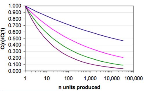
efficiency is εb ~0.8, for millimeter wave beams at ~100 GHz, εb ~0.4, but for lasers, can be εb3.4 Economies of Scale, Learning Curve The components we’re modeling here, antennas and sources of microwave, mm-wave and laser beams, will be produced in large quantities for the large scales of directed energy-driven sails. High-volume manufacturing will drive costs down. Such economies of scale are accounted for by the learning curve, the decrease in unit cost of hardware with increasing production, shown in Fig. 3. This is expressed as the cost reduction for each doubling of the number of units, the learning curve factor f. This factor typically varies with differing fractions of labor and automation, 0.7
For example, for a 90% learning curve, the cost of a second item is 90% of the cost of the first, the fourth is 90% of the cost of the second, and the 2Nth item is 90% of the cost of the Nth item. Then the cost of 64 items is 64 times 0.53 C1. Ordered in bulk, the 64 items will cost 47% less than ordered for production one-at-a-time. The CSR is 1.88. Thus, economies of scale reduce cost by larger and larger amounts as systems grow. For the technologies of power beaming systems, it is well documented that antennas and microwave sources have a 85% learning curve, (learning curve factor f=0.85) based on large- scale production of antennas, magnetrons, klystrons and TWTs [21]. For from the above CSR=N0.233, CN = C1N1-‐0.233 = C1N0.767. Note that, because the number of elements of antennas and millimeter wave sources is different, the economies of scale are different, making their equal costs in the basic case (Eq. 12) substantially different when economies of scale are applied to bring down system cost (see Table 2). 4. Starship Examples We work a few example missions, using the methodology developed here, to illustrate how the key features of Starships driven by beamed energy can be deduced from a few requirements in a self-consistent way, resulting in the lowest-cost concept. One then learns what factors drive a specific result. Then the assumed parameters, such as sail diameter, can be varied to get a more attractive system. See Appendix C for the methodology. We consider only flyby probe missions, so no deceleration occurs. The key features are shown in Table 1. The much lower economies-of-scale costs, with learning curve 0.85 taken into account, are in Table 2, based on coefficients in Table 3. Note one of the key challenges of directed energy is the pointing accuracy; i.e., that required to keep the beam on the sail. That parameter is roughly the ratio of the sail diameter to the accelerating distance, DS/R0. 4.1 Interstellar Precursor—2x10⁻⁴c—Getting our Feet Wet What is the cost of a power beaming facility to lunch a probe out of the Solar System? Velocity is assumed to be 63 km/sec, as in studies of precursors [21]. We use the cost coefficients of present day millimeter wave gyrotron systems, p=3$/W, and antennas for ~100 GHz, a=10,000 $/m2. For the sail characteristics, choose the sail mass/area σS = 4 x10⁻⁵ kg/m2, and reflectivity η= 0.9, which are at the optimistic end of the values Matloff provides for a beryllium hollow- body sail [22]. The 1-km diameter sail mass is 31.7 kg. Assume the sail mass equals mP the payload mass, so m=2 mP, total mass is 62.8 kg. Kinetic energy is roughly 1011 J. The beaming system has these derived parameters: Power 38 GW, antenna diameter 3.8 km, optimum capital cost 230 B$ (without economies of scale, which reduce costs by one or two orders of magnitude, see below). The distance over which the sail is accelerated efficiently (Eq. A1) R0 =520,000 km, 12
f the order of the distance to the moon. Acceleration is 2.4 m/s2, a quarter of a gee, and
acceleration time is 5 hours. Pointing accuracy is µradians, present-day capability. So this
mission can be done from a ground array, with power from the Earth grid, from a site with
altitude high enough and humidity low enough that 100 GHZ mm-waves propagate through the
atmosphere with little loss.
To gain economies-of-scale, gyrotron cost scales as the power P, and 1.2 MW units now cost 3.6
M$, or $3/W, including the power supply, in single units. The number of such units needed for
24 GW is 32,000. From Eq. 19, cost of the millimeter wave power will be reduced by economies
of scale to 10 B$. Antennas in the 100 GHz range cost about $10,000/m2, based on the 64 12-m
diameter dishes of ALMA. The number of ALMA-sized elements needed is 1,600. The antenna
cost falls to 19.5 B$. The total capital cost falls from 230 B$ to 30 B$, so cost savings ratio
CSR~8. This is about ten times the cost of the Flagship missions to the outer planets, Galileo
and Cassini.
The operating cost, i.e., the electrical cost to launch out of the Solar System is 41 M$. Once
built, the beaming facility can send many probes into the interstellar medium. The strategy will
be to use the system to launch sequences of sails in many directions to sample the Interstellar
Medium and flyby Kuiper Belt and Oort Cloud objects, such as Senda. As the facility grows, the
sails will be driven faster and can carry larger payloads.
4.2 Starship at 0.1c—Into the Interstellar
This Starship makes the big leap into the Interstellar with speed ~500 times that of the Precursor.
Kinetic energy is 1.8 x 10¹⁸ J. Pointing accuracy becomes tens of nanoradians, beyond present
capability. The acceleration distance is four times the Sun-Earth distance, because of the low
sail diameter. Consequently, the acceleration required is very high, about 80 gees. But from Eq.
4, acceleration is strongly temperature-limited. Not even carbon can survive the heating due to
absorption at this acceleration. Sail reflectivity would have to be close to perfect to allow such
acceleration. How to change this concept, via the assumed parameters, to bring down the
acceleration, is left as an exercise for the reader.

Cost is in the 10 T$ range, even with economies of scale, and is larger than any past human
project.
4.3 Starship at 0.5c—Getting There Fast
Pushing into the relativistic realm, with a gamma factor of 1.15, shows the enormous energies
required: kinetic energy is 4.5 x 10²¹ J. Millis shows that such propulsion energies may not be
available for centuries [23]. Because the sail is relativistic, the force on it will be reduced.
McInnes describes the relativistic relations [2]. The correction is roughly γ/1−β, about a factor
of two. We increase the sail to 100 km diameter; consequently mass becomes 400 tons. Using a
laser, with perfect reflectivity and present-day cost parameters (Table 3), the acceleration is low,
and occurs over half a light year. Consequently, pointing accuracy is very high, much less than a
nanoradian. Capital cost, while high, is only 2.7 times that of the 0.1 c example. Costs of
electricity to drive the laser, albeit at today’s rates, now greatly exceed capital cost. In fact, the
laser is only 0.5% of the cost, so the choice of frequency doesn’t matter.


                                               13
       Starship Concept
           Interstellar                    0.1 c Starship
        0.5 c Starship

                                     Precursor


            Assumed


           Parameters


             velocity
              6.3x10⁴m/s                        3x10⁷m/s
             1.5x10⁸m/s

                                    (63 km/sec)


               mass
                   63 kg
            4,000 kg (4 tons)
           4x10⁵ kg (400 tons)


        Sail diameter Ds
               1 km
                         10 km
                  100 km


            frequency
               100 GHz
                        100 GHz
          3x10¹⁴
  (λ
  =1
  µm)


 Calculated Physical


     Parameters


         kinetic energy             1.25 x10¹¹ J
                    1.8 x10¹⁸ J
            4.5 x10²¹ J


              power
                  38 GW
                         486 TW
                  120 TW


        antenna aperture
            11.4 km2
                      9 103 km2
            1.67 104
  km2


        antenna diameter
             3.8 km
                         430 km
                 146 km


        sail acceleration
           2.4 m s2
                       770 m/s2
                1.9 m/s2


           acceleration           5.2 108m=520,000          6 1011m=3.9AU
                6 1015m= 0.6 ly

             distance
                  km


        acceleration time
          4.6 hours
                       11 hours
               920 days


       pointing
  accuracy
          2
  µ
  rad
                 67 n rad                0.02 n rad

        Efficiency (v/c)
             0.02%
                            10%
                     50%


          Calculated


       Optimized Costs
       w/o economies of
             scale


       Total Capital Cost,             230 B$
                        2900 T$
               33.500 T$

              CC


       Operating Cost, CO
            41 M$
                          1.3 T$
                2,500 T$


          Table 1 Starship concepts parameters. Efficiency is that of conversion of electricity to sail
            kinetic energy. Costs do not include economies of scale, which are given in Table 2.


                                                         14
Economies of Scale Interstellar 0.1 c Starship 0.5 c Starship
Costs Precursor
Power cost 10 B$ 14 T$ 44 T$
Antenna cost 20 B$ 28 T$ 70 T$
Total Capital Cost 30 B$ 42 T$ 114 T$
Cost Savings Ratio 7.7 70 295
Table 2 Starship concepts costs with economies of scale taken into account (Eq.19). Cost
parameters for power and area based on coefficients in Table 3. Operating cost does not change
with economies of scale, see Eq. 18.
5. Observations on Cost-Optimized Scaling
1) Optimum scaling The cost elements, antenna and power source, are both proportional to the
same key features, the velocity, transmitter diameter and frequency:
2/3
⎡ mV 2 ⎤
opt
C C ∝ ⎢ 0
⎥
⎢⎣ Ds f ⎥⎦ (20)
Therefore, cost can be reduced by
• larger sails,
• lower mass sails,
• higher frequency, probably
€ the upper mm wave >100 GHz.
2) Most important cost Note that p, the cost per watt, is more important than a, the cost per
square meter.
C opt ∝ p 2 / 3 a1/ 3
(21)
So, reducing the cost of power will be more important than reducing the cost of antennas.
3) Transit time scaling Flight time to the target star τ is
€
1 1
τ∝ ∝
v0 C opt 3 / 4
(22)
1
C opt ∝
τ 4/3
15
€So, halving the transit time by doubling the speed will cost 2.5 times as much. That’s an
unfavorable scaling.
4) One clear conclusion from these examples is that the high speeds necessary for fast interstellar
missions make the operating cost exceed the capital cost. Missions will not be flown until the
cost of electrical power in space is reduced orders of magnitude below current levels.
5) Power scales like area Note the linear proportionality between the optimal power and optimal
area. To maintain minimum cost while increasing the effective isotropic radiated power, both
must be increased in proportion.
6) Large sail scaling In present-day small sails, mass is mostly payload. But much larger sails
will have most mass in the sail material. For that case, the technology parameter that drives
performance for sails is the area mass density σ, in
kg/m2,
m=
σ As
.
Rewriting
Eq.
12,
2/3
⎡σD V 2 ⎤ 2/3
opt
C C ∝ ⎢ s 0 ⎥ ∝ Ds
⎢⎣ f ⎥⎦
(23)
We should move toward smaller sails with as low an area mass density as possible.
7) Cost vs speed For faster interstellar precursor probes, Eq. 12 means that cost will scale as v4/3.
€
8) Trading off capital vs. operating costs: The ratio of capital cost to operating cost is
2/3 1/ 3
C opt
1 ⎡ mv2 ⎤ ⎡ v ⎤
C
∝ ⎢ ⎥ = ⎢ ⎥
⎢⎣ mDs ⎥⎦
(24)
2
Co mv ⎣ Ds ⎦
Note this does not include economies of scale. If the sail dominates the mass, as would likely
occur for more advanced missions,
m=
σ πDs2/4,
and the scaling becomes
€ 1/ 3
C opt ⎡ v ⎤
C
∝ ⎢ 2 ⎥
(25)
C o ⎣ m ⎦
So, the designer can shift the cost to the operating budget by decreasing speed, or increasing
mass, either by increasing payload mass or, and most likely, sail diameter.
€
16
5.1 Frequency Figure of Merit
What is the ‘right’ frequency for directed energy? Advocates of microwaves point to that fully
developed, low-cost technology that propagates easily in atmosphere and vacuum. Millimeter-
wave proponents favor present-day high average power capability and better focusing due to
higher frequency, although it propagates with little loss only in certain ‘windows’ in the
atmosphere. Laser fans feel that technology will win out because of the much higher frequency
leading to much smaller optical elements, though propagation is poor in atmosphere at high
intensity.
Here we propose a Figure of Merit (FOM) for directed energy based on cost. The frequency-
dependent factors in the optimized capital cost are, from Eq. 12:
1/ 3
⎡ p 2 a ⎤
opt
C ∝ ⎢ 2 ⎥ ≡ FOM (26)
⎣ f ⎦
Table 3 shows three technologies, and the Figure of Merit. The laser technology is a fiber laser
with 20% electrical efficiency. Gyrotrons have 50% efficiency with direct converters,
magnetrons can be 90% € efficient.
Technology
Power cost Aperture Cost Frequency
Figure of Merit
p
a
Magnetron
1 $/W
1000 $/m2
1-10 GHz
2
Gyrotron
3 $/W
10,000 $/m2
100 GHz
2
Laser
140 $/W
1M$/m2
3 1014 Hz (1
µ
m)
1.25
Table 3 Capital cost Comparisons of Technologies. Figure of Merit is in units of 10-6 $-sec/W-
m2. Millimeter and laser data courtesy of Kevin Parkin and Creon Levit. Costs are based on a 1
MW magnetron, 1 M$ unit, millimeter wave 1.2 MW unit at 3.6 M$, and a 1 kW, 1 micron fiber
laser bought for 140 k$. Antenna costs basis are satellite dishes for microwave, 64 ALMA 12-m
diameter dishes, and 1-m optic at 1 M$.
Remarkably, the technologies have equal capital cost figures of merit at today’s costs. The
focusing advantage of lasers is cancelled by the high cost of both the laser and the aperture
(sometimes called beam director’, ‘telescope’). But note the high electrical costs of driving
lasers, due to their low efficiency (Table 1) also makes them have a much larger total (capital
plus operating) cost. Consequently, the total cost of millimeter wave systems is lower.
Microwave technology is well developed, and has good costing data. Millimeter wave is a
younger technology than lasers; the millimeter market is just beginning to develop so the costs
17
are evolving. High power continuous lasers, after developing quite slowly, are beginning to see
prices drop, but still do not have a clear market. They may soon reach a firm price point. At
present, the cheaper microwave and millimeter wave are readily available. They are much easier
to use for experiments, so those experiments are more likely to be done. Consequently, they are
likely to become more practical.

Of course, future cost changes will determine the most cost-effective technology.

6.0 Development Path for Directed Energy Propulsion

To eventually have a directed energy capability, space infrastructure must exist to build on. How
do we get from where we are now to a future when directed energy can be used for fast missions,
including interstellar? By developing solar sails and other applications of directed energy in
parallel.

6.1 Solar Sail Development

Recent papers by Friedman and Matloff in this Symposium have shown a path for solar sail
technology to lead to speeds on the scale of the Interstellar Precursor described in 4.2 [23-25].
Such development directly enables directed energy sails:

       •   Sail engineering, especially materials: carbon nanotubes,, carbon microtruss
       •   As sails are large-scale structures in space, they also influence the development of large
           transmitting antennas.

This leads to:
   • Larger sails,
   • Lighter sails,
   • Faster sails
   • Fast Solar Sail Missions, for example to the Oort Cloud, Heliopause, and Interstellar
        Medium

This prepares the ground for Beam Propulsion.

6. 2 Development of Directed Energy Propulsion

Power beaming becomes economic only when it can move power from where it is cheap and
accessible to places where it is hard to come by. Previous work has shown that it is often more
economical to transmit power than to move the equipment to produce power locally. Modern
power systems are complex, but if power for space can be located where it is easily accessible
and adjacent to where the required skilled people are located, i.e., on Earth, then it becomes more
practical.
Applications can be met by building up a system existing technologies: microwave and
millimeter wave antennas are already in use for astronomy, gyrotron sources at high frequencies


                                                  18
(>100 GHz) are being developed for fusion. The method is to build, stairstep-like, a sequence of
applications of beaming power [18]:

       •   Orbital debris mapping could be the first objective.
       •   Recharging of satellite batteries in LEO could be economic [26], followed by recharging
           of satellites in GEO.
       •   Launch into orbit of 1000 kg cargo-carrying supply modules makes industrial transport in
           and out of LEO a reality at cost about an order of magnitude less than present day [27].
In today's frugal climate, it is important for technology development to be coupled to commercial
applications. Several of the missions we've described are potentially commercial matters.
Starting with orbital debris mapping, one can see an incremental commercial development
leading first to satellite power recharging. Eventually, as the space market and business
confidence grows and capital becomes more available, this development plan leads to the
repowering of satellites in GEO and ultimately to launch services. Investment costs are
minimized because the research program leads to many applications.
Therefore, the private sector should be included from the outset in the development of power
beaming for space applications. This includes the R&D phase, as it is very important to gain
support from industry to maintain a long-term commercial strategy.
There is at present no clear view of how it is to be achieved and by what technology we are to
make the Solar System readily accessible. This paper has attempted to demonstrate that the
technical means are already in hand for a space infrastructure. A unified approach to many
missions can be found by looking to the use of microwave, millimeter wave and laser beams to
provide power and transportation. Interplanetary infrastructure development will be treated
further in the forthcoming book Starship Century [28].

7. Conclusions

Microwave propelled sails have no physics issues and offer much lower cost probes. Its large-
scale antenna and powerful radiator mean the questions to face are engineering and cost.
Relations have been derived here for quantifying this question, including economies of scale
(‘learning curve’). One clear conclusion from examples shown here is that the cost of interstellar
sailships is very high, driven by current costs for electrical power, radiation source and antennas.
The high speeds necessary for fast interstellar missions make the operating cost exceed the
capital cost. Missions will not be flown until the cost of electrical power in space is reduced
orders of magnitude below current levels.

The usefulness of the beamed power/sail method awaits further quantification by:

       •   Analyzing past concepts (Forward, Landis, Frisbee, Matloff) to see if they are off-
           optimal, so can be improved.
       •   Searching for the lowest cost missions by exploring parameter variations of the physical
           parameters.


                                                 19
•   Quantifying an alternate use of sails-deceleration of sail probes from a fusion-powered
           starship as it approaches stellar systems.


8. Acknowledgments I gratefully acknowledge data from Kevin
  Parkin
  and
  Creon
  Levit and
discussions with Greg Matloff, Greg Benford and Geoff Landis.

9. References

1. D. Price, J. Levine, and J. Benford, “ORION-A Frequency-Agile HPM Field Test System”,
Seventh National Conference on High Power Microwave Technology, Laurel, MD, 1997.
2. C. McInnes,, Solar Sailing: Technology, Dynamics, and Mission Applications, Springer-
Verlag, NY, 1999.

3. R. L. Forward, "Roundtrip Interstellar Travel Using Laser-Pushed Lightsails", J. Spacecraft
and Rockets, 21, pp. 187-195, 1984.
4. R.L. Forward, “Starwisp: an ultra-light interstellar probe”, J. Spacecraft and Rockets, 22, pp.
345-350, 1985.
5. J. Benford and G. Benford, “Flight Of Microwave-Driven Sails: Experiments And
Applications”, Beamed Energy Propulsion, AIP Conf. Proc. 664, pp. 303-312, A. Pakhomov,
ed., 2003.

6. E Schamiloglu, “3-D Simulations Of Rigid Microwave Propelled Sails Including Spin”, Proc.
Space Technology and Applications International Forum, AIP Conf. Proc. 552, 559, 2001.

7. G. Benford, O. Goronostavea and J. Benford, “Experimental Tests Of Beam-Riding Sail
Dynamics”, Beamed Energy Propulsion, AIP Conf. Proc. 664, pp. 325-335, Pakhomov A., ed.,
2003.
8. G. Benford and P. Nissenson, “Reducing Solar Sail Escape Times From Earth Orbit Using
Beamed Energy”, JBIS, 59, pp. 108-111, 2006.
9. T. R. Meyer, C. P. McKay, P.M. McKenna and W.R. Pyror, "Rapid Delivery of Small
Payloads to Mars", AAS Paper AAS-84-172, The Case for Mars II, pp 419-431, C.P. McKay,
Ed., Vol. 62 of the Science and Technology Series, Am. Astronomical Society, 1985.
10. J. Kare, "Beamed Power Missions to Jupiter", Presented at the Space Exploration and
Development Horizon Mission Methodology Workshop, Jet Propulsion Laboratory, Pasadena
CA, September 22-23, 1994.
11. G. Benford and J. Benford, “Power-Beaming Concepts For Future Deep Space Exploration”,
JBIS, 59, pp. 104-107, 2006.
12. G.A Landis, "Small Laser-Propelled Interstellar Probe”, JBIS, 50, pp 149-154, 1977.
13. G.A Landis, "Optics and Materials Considerations for a Laser-Propelled Lightsail”, IAA
Paper IAA-89-684, Presented at the 40th Congress of the Intl. Astronautical Federation, 1989.


                                               20
14. G.A Landis, “Beamed Energy Propulsion For Practical Interstellar Flight”, JBIS, 52, 420,
1999.
15. G.A Landis, “Microwave-Pushed Interstellar Sail: Starwisp Revisited”, paper AIAA-2000-
3337, 36th Joint Propulsion Conference, 2000.

16. R.H. Frisbee, “Limits of Interstellar Flight Technology”, in Frontiers of Propulsion Science,
Vol. 227, ed. M. G. Millis and E. W. Davis, Progress in Astronautics and Aeronautics, AIAA
Press, Reston VA, p.31, 2009.
17. J. Benford, D. Benford and G. Benford, “Messaging With Cost Optimized Interstellar
Beacons”, Astrobiology, 10, pp. 475-491, 2010. Also at arxiv.org/abs/0810.3964v2
18. J. Benford and R. Dickinson, Space propulsion and power beaming using millimeter systems,
Proc. SPIE, 2557, pp. 179-193, 1995. Also published in Space Energy and Transportation, 1,
211, 1996.
19. J. Kare, and K. Parkin, “Comparison of laser and microwave approaches to CW beamed
energy launch” In Beamed Energy Propulsion-2005, K. Komurasaki, ed., AIP Conf. Proc. 830,
New York: Am. Inst. of Physics, pp. 388-399, 2006.
20. N. Luhmann, et al., “Affordable Manufacturing”, Modern Microwave and Millimeter-Wave
Power Electronics, Ch. 14, ed. R. Barker et al, IEEE Press, Piscataway, N.J., pp.731-764, 2005.

21. P.C. Liewer, R.A. Mewaldt, J.A. Ayon, C. Gamer, S. Gavit, R.A. Wallace, “Interstellar probe
using a solar sail: conceptual design and technological challenges”, in: K. Scherer, H. Fichtner,
H.-J. Fahr, E. Marsch (Eds.), COSPAR Colloquium on The Outer Heliosphere: The Next
Frontiers COSPAR Colloquia Series, Pergamon Press, New York, pp. 411–420, 2001.
22. G.L. Matloff, “The Beryllium Hollow-Body Sail and Interstellar Travel”, JBIS, 59, pp. 349-
354 2006.
23. M. Millis, “First Interstellar Missions, Considering Energy and Incessant Obsolescence”,
JBIS, 63, pp. 434-443, 2010.
24. L. Friedman, D. Garber, and T. Heinsheime, “Evolutionary Lightsailing Missions for the
100-Year Starship”, JBIS. Submission pending, 2011.
25. G. L. Matloff, “Interstellar Light Sails”, JBIS. Submission pending, 2011.
26. Y. K. Bae, ‘Photonic Railway: “A Sustainable Developmental Pathway Of Photon
Propulsion”, JBIS. Submission pending, 2011.
26. M., Miller G., Kadiramangalam M. and W. Ziegler, “Earth-to-satellite microwave power
transmission”, J. of Propulsion & Power, 5, pp. 750, 1989.
27. K. Parkin, L.D. DiDomenico and F.E.C. Culick, The microwave thermal thruster concept, in
AIP Conf. Proc.702 Second international symposium on beamed-energy propulsion, Komurasaki
K., Ed., Melville NY, 418, 2004.


                                             21
28. G. Benford and J. Benford, Starship Century, in press, 2013.

Appendix A

Cost Optimization


Examples of how cost optimization can make a big difference:

1) Interstellar Beacons We used this method to quantify the cost of interstellar beacons, the
subject of SETI. The result shows that there is a sharp cost optimum, as in Figure A1.

Fig. A1a. Antenna, microwave power and total costs of Beacon of EIRP=1017 W, antenna cost
k$/m2, power cost p=3 $/W, at f=1 GHz. Note: minimum total cost is at the point where the


                                              22
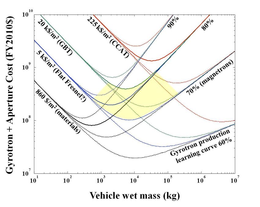
antenna cost and power cost are equal. Fig. A1b. Impact of pulsed sources on system cost of
Beacons of EIRP=1017 W. Cases of long-pulse sources at 3$/W (same as Fig. A1a case) and
short-pulse sources at 0.3$/W and 0.03$/W. [17]

2) Beamed Energy Launcher It is possible to estimate the size of a millimeter-wave beam-driven
rocket, which minimizes beam facility cost. This minimum occurs at a balance between two
opposing expenses: the antenna/optics and the millimeter wave power (Fig. 2).

Fig. A2. Tradeoff in minimizing cost of millimeter wave beam-driven rocket shows that cost-
optimization makes a big difference (K. Parkin, private communication). Note that cost
optimized (minimized) cost implies minimized mass as well, as antenna area and beamed power
are proportional to both cost and mass.

Appendix B

Sail Starship Equations of Motion


For a beam-driven sail, at what range does the beamwidth size exceed the sail size? If power is
constant in time, what speed is attained at this point? How much more speed results if the beam
remains on beyond this point?
When the diameter of the sail Ds is equal to the spot size of the beam at R0,


                                              23
2.44 λ/ Dt = Ds/R0, (A1)
R0 = Ds Dt/2.44λ
Note that at this point power transfer can be quite efficient. Force on the sail will be constant out
to R0, and then will fall off as R-2. Denote the force for R< R0 as
F0=[η +1] P/c, where P is the
power,
η
the reflectivity. To find the speed at any range, solve the equation of motion and solev
for the constant force region and that where force varies as 1/R:
dv dv dr dv F
a= = =v =
dt dr dt dr m
(A2)
R F(R)
∫ 0 vdv = ∫ 0
v
dr
m
€
F = F0 , R < R 0
€
2,
⎛ R ⎞
(A3)
F = F0 ⎜ 0 ⎟ , R > R 0
⎝ R ⎠
For R=R0,
€ v2 0 F0 R 0
=
2 m
(A4))
2F0 R 0 2(η + 1) PR 0
v0 = =
m mc
For R>R0,
∞ 2
vf F0 ⎛ R0 ⎞
€ ∫ v0
vdv = ∫ ⎜ ⎟ dR
m ⎝ R ⎠
R0
2
vf v 0 2 ⎛ F0 2 ⎞⎡ 1 1 ⎤ F0
− = ⎜ R ⎟⎢ − ⎥ = R
2 2 ⎝ m 0 ⎠⎣ ∞ R0 ⎦ m 0 (A4)
F0 R0 (η +1)PR0
vf = 2 =2 = 2v 0
m mc
€
24
Continuing to drive the sailship beyond R0 makes sail velocity increase by 21/2 -1=41%. The
energy can be doubled if the sail is accelerated far beyond R0. But the efficiency gradually falls
as the beam gets ever larger than the sail.


                                              25
Appendix
C
Sail
Starship
Design
Methodology.
The
concepts
in
Table
1
are
derived
from
the
optimization
relation
(Eq.
12)
and
kinematics.
The
procedure
is:
Assume
Key
Parameters
1)
Assume
velocity
v
and
mass
m.
2)
Assume
sail
diameter
Ds.
This
is
important
because
1)
It
should
fit
with
the
area
mass
density
σ,
m=σ A.
See
fifth
remark
in
Section
5.
2)
From
Eqs.
3
and
12,
acceleration
a~1/D2.
A
small
sail
can
give
accelerations
sufficient
to
melt
or
sublime
the
sail
material,
so
estimate
the
limiting
acceleration
and
stay
below
it.
As
this
involves
Eq.
14,
you
may
have
to
iterate.
3)
Assume
a
frequency
domain.
Note
that
assigns
the
cost
parameters
for
power
and
area,
p
and
a
(Eq.
5,
Table
2).
Calculate
Physical
Parameters
4)
Calculate
kinetic
energy
KE
(=mv2/2)
5)
Calculate
optimized
cost
(economies
of
scale
costs
are
calculated
later)
from
Eq.
12.
6)
Calculate
optimum
area
(and
diameter)
and
power
from
Eqs.
13
and
14.
7)
Calculate
acceleration
from
Eq.
3.
8)
Calculate
range
R0
from
Eq.
A1.
9)
Calculate
acceleration
time
(beam-‐on
time)
from
2R 0
t=
(A5)
a
Calculate
Costs
10)
Calculate
operating
cost
from
Eq.
18.
€
11)
Calculate
economies
of
scale
from
Eq.
19.
The
key
parameter
is
N,
which
is
either
the
number
of
sources
(Ns)
or
the
number
of
antenna
(optic)
elements
(Na).
Use
the
data
from
Table
2.
12)
Calculate
a
reduced
capital
cost
from
economies
of
scale
by
adding
results
of
10)
and
11).
26
You can also read