Hydrothermal Carbonization Kinetics of Lignocellulosic Agro-Wastes: Experimental Data and Modeling - MDPI
←
→
Page content transcription
If your browser does not render page correctly, please read the page content below

Article

Hydrothermal Carbonization Kinetics of
Lignocellulosic Agro-Wastes: Experimental Data
and Modeling
Michela Lucian, Maurizio Volpe and Luca Fiori *
 Department of Civil, Environmental and Mechanical Engineering, University of Trento, Via Mesiano 77,
 38123 Trento, Italy; michela.lucian@unitn.it (M.L.); maurizio.volpe@unitn.it (M.V.)
 * Correspondence: luca.fiori@unitn.it; Tel.: +39-0461-282692

 Received: 11 December 2018; Accepted: 1 February 2019; Published: 6 February 2019

 Abstract: Olive trimmings (OT) were used as feedstock for an in-depth experimental study on the
 reaction kinetics controlling hydrothermal carbonization (HTC). OT were hydrothermally
 carbonized for a residence time τ of up to 8 h at temperatures between 180 and 250 °C to
 systematically investigate the chemical and energy properties changes of hydrochars during HTC.
 Additional experiments at 120 and 150 °C at τ = 0 h were carried out to analyze the heat-up transient
 phase required to reach the HTC set-point temperature. Furthermore, an original HTC reaction
 kinetics model was developed. The HTC reaction pathway was described through a lumped model,
 in which biomass is converted into solid (distinguished between primary and secondary char),
 liquid, and gaseous products. The kinetics model, written in MATLABTM, was used in best fitting
 routines with HTC experimental data obtained using OT and two other agro-wastes previously
 tested: grape marc and Opuntia Ficus Indica. The HTC kinetics model effectively predicts carbon
 distribution among HTC products versus time with the thermal transient phase included; it
 represents an effective tool for R&D in the HTC field. Importantly, both modeling and experimental
 data suggest that already during the heat-up phase, biomass greatly carbonizes, in particular at the
 highest temperature tested of 250 °C.

 Keywords: hydrothermal carbonization (HTC); reaction kinetics; modeling; carbon recovery;
 activation energy; agro-wastes; olive trimmings

1. Introduction
     In the last few decades, the need to find new environmentally friendly and sustainable
technologies to produce clean energy from waste biomass has inspired scientific research to study
and develop more efficient and reliable tools for waste biomass exploitation. Among these
technologies, pyrolysis of agricultural and agro-industrial waste has received particular attention
from the points of view of process dependent bio-char properties [1–3], pyrolysis kinetics [4,5], and
innovative technology development [6]. Due to the high-energy needs of converting moist waste
biomass through conventional dry pyrolysis, a wet pyrolysis technology, known also as
hydrothermal carbonization (HTC), has gained increasing attention in the last few years. HTC is a
wet thermochemical process carried out at relatively mild conditions: temperatures between 180 and
280 °C, autogenous saturated vapour pressure between 10 and 80 bars, and residence time ranging
from a few minutes up to several hours. Under these process conditions, water acts similarly to an
organic solvent due to the tremendous changes in its polarity and dielectric constant, and as a catalyst
for biomass conversion via hydrolysis, dehydration, and decarboxylation reactions [7–11]. The main
product of HTC is a carbon-rich solid material referred to as hydrochar, which finds application as

Energies 2019, 12, 516; doi:10.3390/en12030516                                www.mdpi.com/journal/energies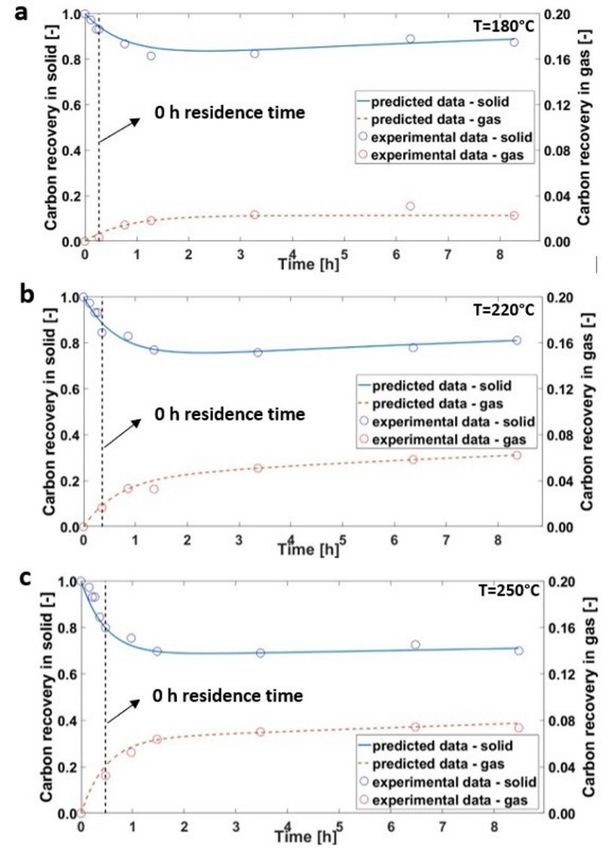
Energies 2019, 12, 516                                                                               2 of 22

high energy bio-fuel [12–21], as a pre-treated material for anaerobic digestion enhancement [15,22],
as a soil amendment [14,23,24], and as an advanced carbonaceous material [25,26]. The high interest
in this wet thermochemical technology, due to its high energy efficiency, relatively mild process
conditions, and scalability, has also been testified by the study on its application at the industrial level
[27,28]. Among different wet residual biomasses, agro-industrial wastes have received particular
attention by HTC scientists due to their large production, high management and treatment costs, and
the potential sanitary and pollution hazards deriving from their improper disposal. In particular,
olive oil milling residues, olive pulp [16,29,30], olive stones, olive mill waste water [31], and their
mixture [14] have been deeply investigated. Much less attention has been focused on the treatment
of olive tree pruning residues [32]. Olive collection and seasonal olive tree pruning produce large
amounts of wet lignocellulosic material not suitable for combustion in stoves and biomass boilers,
and is therefore commonly abandoned and burnt in open fields with negative consequences to the
soil and air quality. This paper reports a comprehensive investigation on HTC conversion of olive
tree pruning residues showing the possibility to produce a valuable carbon-rich solid biofuel.
      If, on the one hand, many research groups have focused their studies on HTC reaction of
different biomasses primarily to determine the influence of process parameters on hydrochar’s
chemical and physical properties, on the other hand, the kinetics of HTC of biomasses and its
modeling still lacks of a deep investigation [33,34]. The HTC reaction mechanism is very complex
and involves several pathways such as hydrolysis, dehydration, decarboxylation, aromatization, and
condensation [35,36]. The complexity of the HTC reaction mechanism has led some authors to
develop lumped kinetics models to describe it. Liu and Balasubramanian considered HTC process as
a unique first order reaction and estimated the activation energy for coconut fibres (67.5 kJ/mol) and
eucalyptus leaves (59.2 kJ/mol) [37]. By using a different approach, Reza and co-workers formulated
a simple reaction mechanism in which hemicellulose and cellulose degrade in parallel while lignin
was assumed to be inert at the temperatures investigated (200–260 °C) [38]. The model developed by
these authors allows for the determination of activation energies of hemicellulose and cellulose
degradation first-order reactions, which were determined to be 30 and 73 kJ/mol, respectively [38].
HTC kinetics of biomass macro-components was also recently reported [39,40]. Jung and Kruse used
an Arrhenius-type overall kinetics equation to model hydrochar mass yield and carbon and oxygen
content for several types of biomasses [34]. Baratieri et al. proposed a kinetics model for HTC based
on a two-step reaction mechanism [41]. They assumed that the original biomass (A) forms an
intermediate product (B) that partially degrades to form the final product C (the hydrochar). In the
meanwhile, two reactions in parallel to those giving compounds B and C take place leading to the
formation of volatiles products. They calibrated their model using HTC experimental data of solid
yields and determined the activation energies and pre-exponential factors of the reactions involved
[41]. Jatzwauck and Schumpe proposed an example of a lumped model describing the HTC
mechanisms [33]. According to the authors, the HTC reaction mainly occurs in three steps: in the first
step, the biomass components are hydrolysed into dissolved intermediates; in the second step, the
intermediates may undergo further reaction in the liquid phase or evolve into gaseous products; in
the last step, alternatively to step two, the intermediates could polymerize to form secondary char. In
their model, the authors also reported carbon distribution among the HTC products [33]. Such a
kinetics model does not take into consideration the direct solid–solid dehydration reaction leading,
as well as polymerization, to char formation. In contrast, some authors [16,42,43] experimentally
demonstrated that hydrochar formation takes place through two reaction pathways: (1) solid–solid
conversion, in which carbonaceous material (primary char or simply char) results predominantly
from dehydration of the parent biomass; and (2) a polymerization reaction, in which a carbonaceous
solid is formed via reactions of back polymerization of organics dissolved in the liquid phase.
      Based on these previous studies, this work reports an original kinetics model assuming that the
HTC process follows a simplified mechanism including both pathways of hydrochar (primary and
secondary char) formation. The model is calibrated on HTC experimental data of olive trimmings
specifically obtained for this purpose, and is further validated with additional HTC data previously
obtained using grape marc [44] and Opuntia ficus indica cladodes [7]. By means of the modeling tool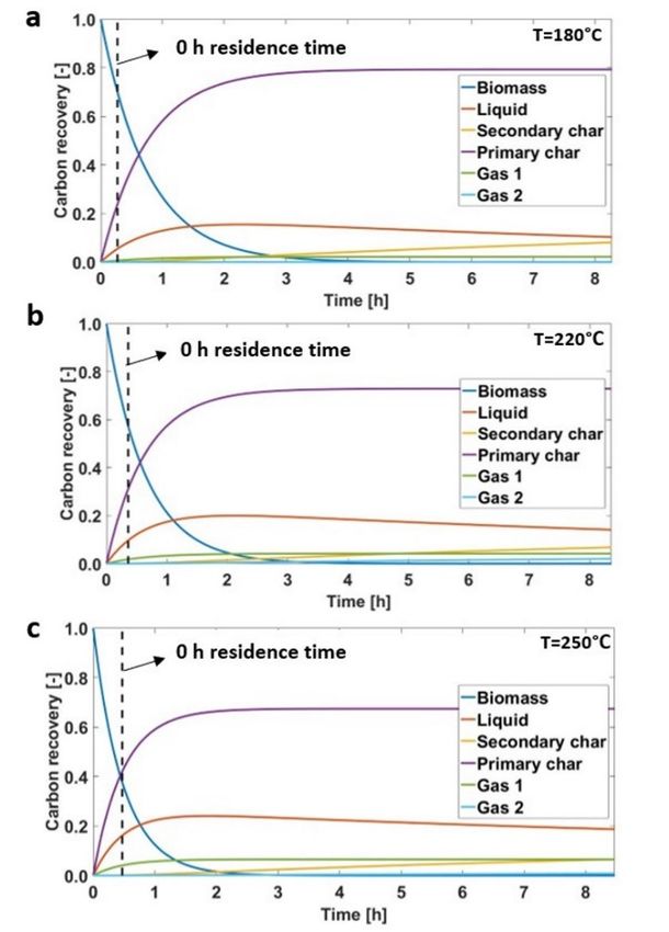
Energies 2019, 12, 516                                                                           3 of 22

developed, the Arrhenius kinetics parameters (pre-exponential factor and activation energy) were
estimated for the reactions constituting the model and for the various biomasses.
     As a whole, this work addresses HTC reaction kinetics of lignocellulosic residual biomasses from
both theoretical and experimental viewpoints, also paying attention to the heat-up transient phase
necessary to increase the HTC reactor temperature to the set point value. Importantly, only in micro-
autoclaves can the time necessary for the system to reach set point HTC temperature be neglected:
for the bench scale and industrial scale applications, it cannot. Nevertheless, to the best knowledge
of the authors, the characterization of the solid product during the heat up phase has never been
addressed before: the study of such a transient phase represents a novelty in the literature.
     To sum up, the present work aims to:
     (1) Analyse the differences in chemical and energy properties of hydrochar versus time at
different HTC temperatures.
     (2) Understand the evolution of hydrochar characteristics during reactor heating time.
     (3) Present an original reaction kinetics model as a tool to predict the carbon distribution among
HTC products: hydrochar (primary and secondary char), gaseous, and liquid phases.

2. Materials and Methods

2.1. HTC Tests
      Olive trimmings, including leaves, were collected from three different 30-year-old olive trees of
the “Moresca” variety in Enna province, Italy. The biomass was dried in a ventilated oven at 105 °C
for 24 h and milled to a particle size lower than 1 mm. To ensure homogeneity, raw material was
sieved and a particle size range between 425 and 850 μm was selected for HTC tests. The HTC set up,
the biomass preparation, and experimental procedures followed in the experimental campaign were
fully described in previous studies [16,45]. For each HTC run, 5 ± 0.01 g of an oven-dried olive
trimmings (OT) sample were loaded into the reactor together with 20 ± 0.01 g of deionized water with
a dry biomass to water ratio (DB/W) equal to 0.25. HTC tests on OT were performed at temperatures
of 180, 220, and 250 °C. Residence times were varied at 0, 0.5, 1, 3, 6, and 8 h. Residence time started
to be counted when the HTC reactor reached the selected HTC set point temperature. Thus, a
residence time of 0 h indicates that the HTC reactor was promptly cooled down as soon as the set
temperature was reached. Cooling was performed by placing the HTC reactor on a cold stainless-
steel mass at −30 °C and blowing fresh compressed air on its external walls. Once the reactor reached
room temperature, its outlet valve was opened to let the gas produced flowing into a graduated
cylinder filled with water [46]. By using this system, the volume of the gas evolved during HTC
reaction was determined. The reactor was then opened, and the solid fraction recovered via filtration.
Finally, the solid residue was dried in a ventilated oven for 8 h at 105 °C. The HTC runs were carried
out in duplicate. The hydrochar yield (Y ), or solid yield, was determined through Equation (1),
where m is the mass of hydrochar (on a dry basis) and m is the mass of the raw biomass (on a
dry basis):
                                                       m
                                              Y    =                                                (1)
                                                       m
     The gas yield was calculated as the ratio of gas produced (mass on a dry basis) and the raw
biomass (mass on a dry basis). As is well-known [28,44,47], CO2 is the main gas produced during
HTC, representing 90–95 vol.% of the total gas. For this reason, the mass of the gas produced was
calculated considering it as solely consisting of CO2. The liquid yield was calculated as the
complement to one of the sum of solid yield and gas yield.
     The energy yield (EY) of hydrochars was calculated as follows:
                                                       HHV
                                            E =Y                                                    (2)
                                                       HHV
where HHV and HHV (MJ/kg) are the higher heating values (on a dry basis) of hydrochar and
raw biomass, respectively.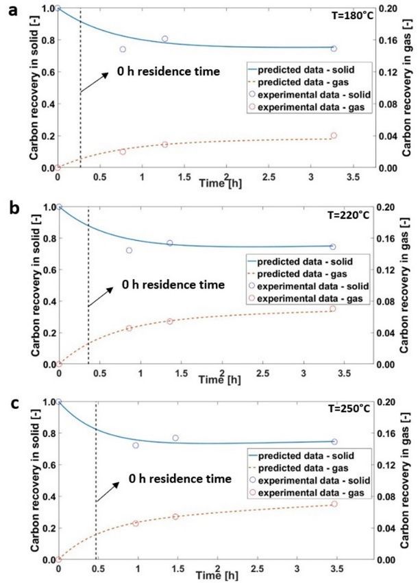
Energies 2019, 12, 516                                                                               4 of 22

2.2. Analytical Determinations
     Ultimate analyses were performed using a LECO 628 analyser (LECO Corporation, St. Joseph,
MI, USA) equipped with sulphur module for CHN (ASTM D-5373 standard method) and S (ASTM
D-1552 standard method) content determination.
     Proximate analyses were carried out by a LECO Thermo-gravimetric Analyser TGA 701
(LECO Corporation, St. Joseph, MI, USA). Moisture content (M), volatile matter (VM), and ashes of
solid samples were respectively determined using the following thermal methods (modified from
ASTM D-3175-89 standard method): 20 °C/min ramp to 105 °C in air, held until constant weight
(
Energies 2019, 12, 516                                                                              5 of 22

thermocouple inside the batch reactor, include both transient time up to the set hydrothermal
temperature and the following immediate cooling down of the apparatus.

2.4. Kinetics Model
    The HTC reaction mechanism was described schematically using a lumped component model
in which the initial feedstock converts into products and intermediates in different steps (Figure 2).

                         Figure 2. Simplified HTC reaction path used in the model [50].

     Reaction 1 (biomass→liquid) refers to a hydrolitic processes leading to the formation of a HTC
liquor rich in intermediate molecules [51] deriving from biomass structural components (extracts,
lignin, cellulose, and hemicellulose). The extracts and hemicellulose constituents are known to be
susceptible to hydrolysis at quite low HTC temperatures (as low as 200 °C) [52]. The
hydrolysis/dissolution of these biomass components leads to oligomers and monomers formation in
the aqueous liquid phase [36]. Similarly, a portion of amorphous cellulose and soluble lignin is
fragmented into smaller molecules, mainly 5-Hydroxymethylfurfural (5-HMF) and phenolic
derivatives [53]. The resulting water-soluble components are very reactive and could undergo a series
of oligomerization/polymerization and/or condensation reactions to form a solid residue referred to
as secondary char (also called polymerized char or coke—Reaction 5, liquid→secondary char). These
reactions are accompanied by decarboxylation and decarbonylation reactions to form CO2 and CO
(Reaction 4, liquid→gas 2). During HTC, the non-dissolved cellulose and lignin contained in biomass
undergo dehydration and decarboxylation/decarbonylation reactions to form an interconnected
network called primary char (or polyaromatic char—Reaction 3, biomass→primary char) [54] and
CO2 and CO (Reaction 2, biomass→gas 1), respectively.
     The reaction rate constants ki (k1, k2, k3, k4, k5) for the five reactions i in Figure 2 are described
within the model by using Arrhenius equation (Equation (3)):

                                       k = k ,e               i = 1, …, 5                             (3)

      The kinetics model consists of a system of six non-linear differential equations, Equations (4)–
(9), representing the carbon molar balances for the different lumped components. C , C , C , C ,
C , and C       are the molar concentration (mol/L) of carbon in biomass (B), liquid (L), gas 1 (G1),
primary char (HC1), gas 2 (G2), and secondary char (HC2), respectively, while t is the reaction time.
It was assumed that all the reactions involved are first order, except the one involving secondary char
formation (Reaction 5, liquid→secondary char). The order of this reaction, also called a
polymerization/condensation reaction, is likely higher than 1 [55]. Thus, in Equation (9), C is to the
power of n, with n ≥ 1, n being the reaction order. The model was also run fixing n = 1; the relevant
modeling results are reported in Appendix A.
                                         ∂C
                                             = −k C − k C − k C                                       (4)
                                          ∂t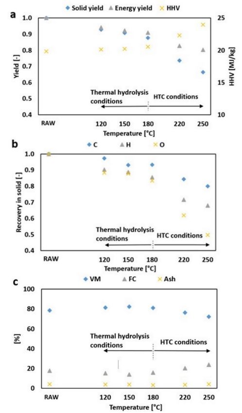
Energies 2019, 12, 516                                                                                                                     6 of 22

                                                       ∂C
                                                           =k C                 −k C −k C                                                    (5)
                                                        ∂t
                                                             ∂C
                                                                                 =k C                                                        (6)
                                                              ∂t
                                                            ∂C
                                                                                 =k C                                                        (7)
                                                              ∂t
                                                             ∂C
                                                                                 =k C                                                        (8)
                                                              ∂t
                                                            ∂C
                                                                                 = k C                                                       (9)
                                                              ∂t
      The carbon molar concentration in component X (B, L, G1, HC1, G2, HC2), C , is given by:
                                                                                  n,
                                                                   C =                                                                      (10)
                                                                                (V + V )
where n , is the number of moles of carbon in component X, and the term V + V is the sum of
the volumes (expressed in L) of biomass and distilled water fed to the HTC reactor to reach the set
DB/W ratio. The kinetics model was written as a MATLABTM software code (MATLAB R2016b
developed by MathWorks Inc., Natick, MA, USA). The differential equations system was solved
numerically using Runge–Kutta method by means of a routine that estimates the kinetics parameters
(k and n) on the basis of experimental data. In more details, the error function F (k , ) represented
by Equation (11), was minimized in order to get k and n by using the Levenberg–Marquardt
algorithm. This “curve-fitting” procedure is a standard tool in computing and it is extensively used
for non-linear least squares problems [56,57].
                         F (k , )= ∑ |C        ,   − C         ,       | + ∑ |C       ,       −C       ,       | + ∑ |C   ,   −C   ,   |    (11)

     Subscripts S, L, and G refer to solid, liquid, and gas phases. The superscript “exp” refers to the
experimental values of the variables obtained at different HTC residence times, while the superscript
“mod” refers to the corresponding values computed by the model. Subscript j is a recursive index for
residence time.
     The experimental data used in model best fitting were obtained using olive trimmings (OT) as
described in Section 2.1, and two others ligno-cellulosic biomasses, namely Opuntia ficus indica
cladodes (OC) and grape marc (GM), tested in previous studies [7,44]. Thus, subscript j refers to the
residence times at which the experimental data were available: six for OT, three for both OC and GM.
     Carbon molar concentrations (C ) using both experimental and modeling data were calculated
and computed through Equations (12)–(16):
                                       n,       m,       1        m %c                                                       1
                         C   ,   =            =     ∙           =                                                     ∙
                                     (V + V )   M     (V + V )     100 M                                                  (V + V )
                                              Y m , %c         1                                                                            (12)
                                            =             ∙
                                                100 M       (V + V )
                                                   C   ,       =C       ,       +C            ,   +C            ,                           (13)
                                                       C   ,       =C       ,    −C       ,       −C       ,                                (14)
                                                 n,      n        PV      1
                                 C    ,   =           =         =      ∙                                                                    (15)
                                              (V + V ) (V + V )    R T (V + V )
                                                           C       ,    =C        ,       +C       ,                                        (16)
     Letters M, m, and Y indicate molar mass (g/mol), mass (g), and solid yield (i.e., hydrochar yield),
respectively. Subscripts c, HC, and 0 refer to carbon, hydrochar, and initial value, respectively. %
indicates the percentage on a dry mass basis.
     In Equation (15), P and T are atmospheric pressure (1 atm) and room temperature (293 K),
respectively; VCO2 is the measured volume of the gas, which was assumed to be 100% CO2, as
discussed in Section 2.1; R is the gas constant (0.08206 L atm/K mol).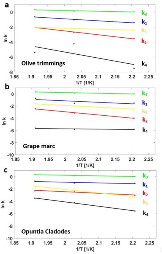
Energies 2019, 12, 516                                                                                7 of 22

     The solid, after the HTC reaction had started, consisted of hydrochar (Equation (12)).
Conversely, in the model (Equation (13)), the solid refers to biomass whose amount decreased during
HTC, while its composition was considered constant (Equation (4)), plus primary char HC1 and
secondary char HC2. In the model (Equation (16)), the gas consisted of the sum of G1 and G2, while
the experimental value was calculated using the ideal gas law (Equation (15)). The experimental
values for the liquid were calculated by difference (Equation (14)), while the relevant model values
were obtained by solving Equation (5). The available experimental data were the input values, V ,
V , m , , and the HTC output values Y , %c (from hydrochar elemental analysis), and V .
Based on the experimental data available for the HTC of OT, (k , ) was minimized for six reaction
times (0, 0.5, 1, 3, 6, and 8 h) at each of the three HTC temperatures tested: 180, 220, and 250 °C. In the
case of GM and OC, the minimization was performed at the same temperatures but by considering
only three residence times (1, 3, and 8 h for GM and 0.5, 1, and 3 h for OC). It is worth mentioning
that in Equation (11), the term related to the liquid phase (which could be actually omitted without
compromising the correctness of the equation) allowed the software to converge faster towards the
solution of the minimization problem. Once the ki values were estimated, the activation energy Ea,i
and pre-exponential factor k0,i for the five simplified HTC reactions of Figure 2 were calculated
through the Arrhenius plot (ln ki vs 1/T).
     Carbon distribution among the HTC products is expressed in terms of carbon recovery (CR),
defined as the ratio of carbon content in each component (n , ) to the carbon content in the raw
biomass (n , , ). The CR parameter allows for an easy understanding of the carbon distribution
among the different HTC phases [58]:
                                                       n,
                                                CR =                                                   (17)
                                                       n, ,
     Similarly, oxygen recovery and hydrogen recovery are defined as the ratio of oxygen (or
hydrogen) content in each component to the oxygen (or hydrogen) content in the raw biomass, on a
dry basis.

3. Results and Discussion

3.1. Hydrothermal Carbonization of Olive Trimmings
      The experimental results relevant to HTC runs performed on OT are summarized in Table 1.
Hydrochar yields decreased with temperature and residence time except for residence times higher
than 3 h. Tests performed at 180 and 250 °C and 6–8 h of residence time showed an increase in
hydrochar yield compared to 3 h residence time, which could be explained by an increased
contribution of back-polymerization at longer residence times [17]. The HHV values progressively
increased with temperature and residence time (except a slight decrease at 8 h). Regarding the
ultimate analysis, the carbon content constantly increased with both time and temperature (except
for 8 h at any temperature), while hydrogen remained approximately constant, with a slight decrease
at the 8 h residence time. As a result of dehydration and decarboxilation, the oxygen content followed
an opposite trend with respect to carbon. As expected, the data showed an increase in fixed carbon
(FC) and a decrease in volatile matter (VM) with temperature. Interestingly, the same trend was
observed when increasing the residence time in the lower residence time range, but for higher
residence times (6–8 h), the trend was reversed.
      All the data of Table 1 in the residence time range 0–3 h presented typical trends reported in the
literature. Of particular interest, in term of reaction kinetics, are the data in the time range 3–8 h. Here,
the hydrochar yield increased; the degradation of primary char was probably more than
counterbalanced by the precipitation in the solid phase of polymerized/condensed organics from the
liquid phase. Hydrochar was enriched in carbon from 3 to 6 h residence time, but lowered its carbon
content at 8 h, when hydrogen content also reduced (and this caused the trend observed for HHV).
Similary, for such a residence time range, FC decreased. This suggests that the precipitation of the so-
called secondary char also led to the presence of thermally instable species, eventually with tar-like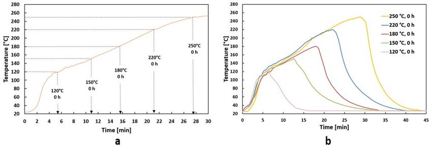
Energies 2019, 12, 516                                                                                                   8 of 22

properties, whose content in carbon was significant in the initial stage of the precipitation (up until 6
h residence time), but less significant thereafter, with precipitation of more oxygenated compounds.

      Table 1. Mass yields, proximate and ultimate analyses, and HHV of raw feedstock and hydrochars.
      Analyses were performed in duplicate. Average values are shown (Er < 2.0% for solid yields; Er <
      3.2% for proximate, and Er < 0.6% for ultimate analyses; Er < 1.0% for HHVs).
                                                       Proximate Analysis             Ultimate Analysis         HHV         EY
   Sample                    Mass Yields (-)
                                                         (wt% on a d.b.)               (wt% on a d.b.)         (MJ/kg)      (-)
                      Solid       Liquid       Gas    VM       FC        Ash    C         H      N      O2
   OT raw                -           -           -    78.4     17.6      4.0   48.3       6.1   1.5     40.0    19.8         -
  120 °C, 0 h          0.93        0.07        0.00   81.3     15.0      3.7   50.6       5.9   1.6     38.1    20.1       0.94
  150 °C, 0 h          0.91        0.09        0.00   82.2     14.0      3.8   49.6       6.0   1.8     38.8    20.2       0.92

 180 °C, 0 h          0.88         0.11        0.01   81.2     15.7     3.1    51.3      5.9     1.6    38.1    20.5       0.91
180 °C, 0.5 h 1       0.78         0.20        0.02   77.3     19.9     2.8    53.7      6.2     1.5    35.7    21.8       0.86
 180 °C, 1 h          0.72         0.25        0.03   76.1     20.3     3.5    54.3      6.1     1.8    34.3    22.6       0.82
 180 °C, 3 h          0.70         0.26        0.04   72.9     23.2     3.9    56.7      6.2     1.8    31.4    23.4       0.83
 180 °C, 6 h          0.73         0.22        0.05   73.8     21.9     4.3    58.9      5.9     1.6    29.2    24.1       0.89
 180 °C, 8 h          0.73         0.23        0.04   76.8     18.0     4.0    57.8      5.3     1.6    31.3    23.7       0.88

 220 °C, 0 h          0.74         0.23        0.03   76.3     20.3     3.5    55.3      5.9     1.5    33.7    22.3       0.83
220 °C, 0.5 h 1       0.71         0.23        0.06   72.9     23.0     4.1    56.3      6.2     1.6    31.7    23.9       0.86
 220 °C, 1 h          0.63         0.31        0.06   70.6     25.1     4.3    59.4      6.2     1.9    28.3    24.7       0.78
 220 °C, 3 h          0.58         0.33        0.09   64.4     31.4     4.2    63.0      6.3     2.2    24.4    26.4       0.77
 220 °C, 6 h          0.57         0.33        0.10   66.9     28.4     4.6    65.5      6.0     2.0    21.8    26.7       0.77
 220 °C, 8 h          0.61         0.28        0.11   70.1     23.6     4.4    64.1      5.5     1.9    24.1    26.7       0.82

 250 °C, 0 h          0.66         0.28        0.06   72.3     23.7     4.0    58.1      6.2     1.6    30.0    23.9       0.80
250 °C, 0.5 h 1       0.58         0.33        0.09   66.3     30.3     3.4    63.2      6.3     1.8    25.3    27.3       0.79
 250 °C, 1 h          0.52         0.37        0.11   66.8     29.2     4.0    65.3      6.2     2.3    22.2    27.8       0.72
 250 °C, 3 h          0.48         0.39        0.12   59.6     35.7     4.7    68.9      6.3     2.5    17.6    29.0       0.71
 250 °C, 6 h          0.50         0.37        0.13   56.3     39.9     3.8    70.6      5.9     2.2    17.5    29.6       0.74
 250 °C, 8 h          0.49         0.38        0.13   61.8     32.0     4.1    69.0      5.5     2.1    19.3    28.9       0.72
                  1   Data from Volpe and Fiori, 2017 [16]; 2 Calculated by difference; d.b.=dry basis

3.2. Hydrothermal Carbonization during Transient Time
     Figure 3 summarizes the experimental results of HTC of OT during the reactor heating up.
Figure 3a shows a slight decrease in solid yield to 0.93 and 0.91 at temperatures typical of thermal
hydrolysis (at 120 and 150 °C, respectively). The drop of solid yield might be explained by the
solubilization of extracts that were quickly extracted from biomass by hot compressed water. With
increasing temperature, at typical hydrothermal carbonization temperatures, solid mass yield
dramatically dropped to 0.74 and 0.66 at 220 and 250 °C, respectively. HHV followed an inverse trend
with respect to solid yield. At temperatures higher than 180 °C, there was a significant increase in
HHV, where there was a substantial decrease in hydrochar yield. The decrease in hydrochar yield
prevailed over the increase of HHV, and thus the energy yield decreased versus temperature.
     Figure 3b shows that, even if carbon percentage in the hydrochar increased with temperature
(ultimate analysis data, Table 1), its recovery lowered, due to the prevailing magnitude of the
hydrochar yield decrease. The decrease of oxygen recovery versus temperature was very large; this
was mainly due to the dehydration reactions occurring during HTC. At the highest temperatures,
decarboxylation also occurred, which resulted in a further significant oxygen release. The hydrogen
recovery mimicked the oxygen recovery in the temperature range typical of thermal hydrolysis,
where dehydratation prevailed. Conversely, hydrogen recovery was greater that oxygen recovery at
the typical HTC temperatures, where decarboxylation prevailed.
     The results of proximate analysis also showed a substantial change in VM and FC at 220 and 250
°C with respect to the lower temperatures (Figure 3c).
     In summary, already during the heating up transient phase, experiments testified to a clear
transition between thermal hydrolysis and HTC. From the collected data, the 180–220 °C range seems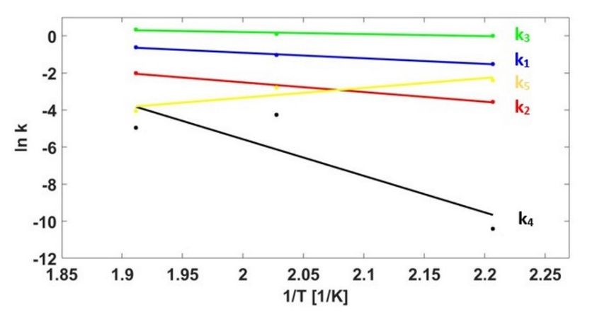
Energies 2019, 12, 516                                                                                      9 of 22

the temperature interval at which this transition occurred. Already during heat up, OT carbonized to
a significant extent if the temperature reached value of 220–250 °C.

      Figure 3. Transient time: (a) hydrochar yield, energy yield, and HHV vs temperature; (b) element
      recovery in the hydrochar vs temperature; and (c) proximate analysis data vs temperature.

3.3. Kinetics Model
    The values of the kinetics parameters estimated using the model for OT, GM, and OC are
reported in Table 2:

      Table 2. Reaction rate constants (ki) and reaction order (n) for the simplified reactions path of Figure
      2.
                     Parameters     Olive Trimmings          Grape Marc        Opuntia Ficus Indica
                       T (°C)      180     220   250     180    220     250     180    220     250
                       k1 (s−1)    0.24   0.35   0.54   0.22    0.21    0.49   0.33   0.35     0.48
                       k2 (s−1)    0.03   0.07   0.14   0.02    0.04    0.09   0.05   0.09     0.10
                       k3 (s−1)    1.05   1.13   1.40   1.00    1.14    1.41   1.04   1.14     1.41
                       k4 (s−1)   0.001 0.014 0.005     0.003 0.003 0.004      0.004 0.015 0.030
                       k5 (s−1)    0.09   0.10   0.14   0.08    0.13    0.20   0.04   0.11     0.21
                        n (-)      1.10   1.51   2.01   1.10    1.51    2.00   1.11   1.51     2.00
Energies 2019, 12, 516 10 of 22
As expected, the rate constants ki increased as the temperature increased for all the feedstocks.
Table 2 shows that k3 was the highest at every HTC condition. Model results suggest that the
conversion of biomass into primary char was the most favoured reaction. The biomass→liquid
reaction was also quite fast, while the reactions involving gas phases were the slowest. Reaction rate
constant k4 was almost negligible compared to the others. The results show that the reaction order n
of secondary char formation increased with temperature. This was in accordance with the results
reported by some other scientists [43].
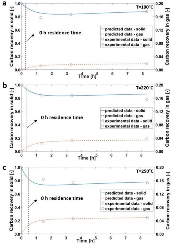
Figure 4 shows the model and experimental CR values in the solid and gas phases for OT. The
vertical dotted lines represent the time for reaching the HTC temperature set point, the time at which
the experimental reaction time had started to be counted. Our simulations, based on the system of
differential equations represented by Equations (4)–(9), conversely considered time zero when the
reactor started to be heated up to reach the set HTC temperature (about 16, 22, and 28 min to reach
180, 220, and 250 °C, respectively; see also Figure 1). While the carbon recovery increased
progressively with time in the gas phase at all the HTC temperatures examined and for all the
feedstocks (see Appendix A—Figures A1 and A2 for GM and OC, respectively), the carbon recovery
in the solid phase decreased during reaction up to about 3 h and then tended to increase or stabilize.
The model fits very well the experimental data; the errors (i.e., the differences between model
predictions and experimental data), calculated by means of Equation (18), were lower than 10% in all
the cases. The error values for all the feedstocks and the plots showing the carbon distribution among
the HTC solid and gas phases for GM and OC are reported in Appendix A (see Table A1, Figures A1
and A2).
|C , − C , |
, = ∙ 100 (18)
C ,
Figure 4. Carbon recovery in solid and gas for olive trimmings: (a) 180 °C, (b) 220 °C, and (c) 250 °C.Energies 2019, 12, 516 11 of 22
Figure 5 reports the carbon recovery in all the six lumped components of the reaction scheme
designed in Figure 2. The carbon recovery plots resulted from the solution of the differential
equations system, Equations (4)–(9), with the optimized kinetics parameters of Table 2. Figure 5 is
relevant to OT.
The carbon recovery curves are of particular interest for the assessment of the kinetics of primary
and secondary char formation, as well as of the gas production from the solid and liquid phases.
Figure 5. Carbon recovery (-) into HTC products versus residence time (h) for olive trimmings: (a) 180
°C, (b) 220 °C, and (c) 250 °C.
The results clearly showed how the initial carbon recovery rate in the liquid (i.e., the slope of the
liquid curve) increased for increasing HTC temperatures. Indeed, at 250 °C, the degradation of
biomass occurred much faster when compared to lower HTC temperatures. At 250 °C, more than half
of the initial carbon content in the biomass moved to HTC products just after the thermal transient
(i.e., at 0 h residence time). The carbon recovery into the liquid phase reached a maximum at
approximately 1.5 h of residence time, after which the gas and, to a lesser extent, the secondary char
seemed predominant. The carbon recovery into the primary char reached a stable value after about 3
h for all the three temperatures. The carbon recovery in secondary char as well as in the gaseous
products increased with time. Such an increase was faster in the gas at the beginning of the HTC
conversion, while the increase in the secondary char was more stable during the course of HTC.
The Arrhenius plots for the different reaction rate constants ki are shown in Figure 6. The
activation energies Ea,i and the pre-exponential factors k0,i for each HTC reactions were determined
from the slope of the curves (−Ea,i/R) and the intercept with the y-axis. The values of the Arrhenius
parameters are reported in Table 3.Energies 2019, 12, 516 12 of 22
Figure 6. Arrhenius plot for determination of the activation energies (Ea,i) and pre-exponential factors
(k0,i): (a) olive trimmings, (b) grape marc, and (c) Opuntia ficus indica cladodes.
Table 3. Pre-exponential factors and activation energies evaluated by the Arrhenius plot for the HTC
reactions for olive trimmings, grape marc, and Opuntia ficus indica.
Parameters Olive Trimmings Grape Marc Opuntia Ficus Indica
k0,1 (s−1) 82.32 41.55 4.31
k0,2 (s−1) 2.51 × 10³ 1.69 × 10³ 14.71
k0,3 (s−1) 7.99 11.28 9.37
k0,4 (s−1) 5.38 × 10⁴ 0.0086 2.40 × 10⁴
k0,5 (s−1) 1.41 52.78 1.14 × 10⁴
Ea,1 (kJ/mol) 22.03 20.23 9.82
Ea,2(kJ/mol) 42.93 43.14 21.33
Ea,3 (kJ/mol) 7.75 9.18 8.39
Ea,4 (kJ/mol) 67.35 4.11 58.92
Ea,5 (kJ/mol) 10.37 24.41 7.44
The activation energies relevant to the formation of primary and secondary char (Ea,3 and Ea,5)
were relatively small in comparison with the activation energies involved in liquid and gas formation,
supporting what was previously reported on the relative rate of the various HTC reaction paths.
However, it is important to point out that the activation energy values here obtained were relevant
to our experimental settings and, consequently, reflected the experimental conditions we used in
terms of water to biomass ratio and, likely even more important, reactor heating rate.
Even if common trends of the kinetic parameters are clearly identifiable in Table 3, some data
appear clearly out of trend. This could be due to a couple of reasons: on the one hand, theEnergies 2019, 12, 516 13 of 22
experimental data available for grape marc and Opuntia ficus indica were quite limited (only three
residence times tested); on the other hand, a clear interrelation existed between pre-exponential factor
and activation energy. Actually, it is worth noticing that the pre-exponential factors followed exactly
the same trend as the activation energies: the higher Ea,i, the higher k0,i. This can be explained by
considering the mathematical aspects behind Arrhenius’s formulation: the interrelations between k0,i
and Ea,i can be expressed as in Equation (19) [59]:
ln k , = aE , +b (19)
Equation (19) highlights that a change in activation energy leads to a change in pre-exponential
factors, and vice-versa. Such a phenomenon can be also related to the so-called compensation effect
[60]. Nevertheless, in general, the results obtained with the Arrhenius plot confirmed that the reaction
leading to the production of primary char was kinetically favoured, the reaction producing gas was
the slowest, and the production of liquid and secondary char occurred at an intermediate rate
compared to the previous ones.
4. Conclusions
Hydrothermal carbonization of olive trimmings showed that product distribution and
hydrochar properties at 180–250 °C were strongly affected by temperature and residence time. The
dependence appeared univocal as far as the temperature is concerned, while residence time affected
in a more complex fashion. As usually found in the literature, the higher the temperature, the lower
the hydrochar yield, and the higher were its HHV, carbon, and fixed carbon. The same applied when
the residence time increased from zero (i.e., the feedstock was heated up to HTC temperature and
then immediately cooled down) to 3 h. Increasing the residence time (HTC tests performed at 6 and
8 h) did not translate into a further decrease in hydrochar yield, which conversely tended to increase
slightly. Carbon content still increased until 6 h residence time, and then stabilized, and fixed carbon
content tended to decrease at the highest residence times tested (6–8 h). This particular behavior can
be explained considering that in the high residence time range, polymerization/condensation
occurred in the liquid phase, and the secondary char and/or tarry compounds segregated from the
liquid phase and precipitated into the solid phase.
An in-depth study on the heat-up transient phase experienced by the feedstock before reaching
HTC set-point temperature also allowed for very interesting results. Results clearly showed a change
in properties during the transient time to 220 and 250 °C: carbonization already began during the
heat-up phase in the 180–220 °C temperature range, and at a corresponding heating time of 15–20
min due to the HTC system utilized. Actually, regarding this temperature range, there was an evident
increase in hydrochar HHV and a substantial decrease in hydrochar yield and oxygen content.
Analyzing the oxygen recovery (a function of both hydrochar yield and oxygen content in the
hydrochar), it seems that, during heat-up, dehydration prevailed until 180 °C, while decarboxylation
became predominant in the temperature range 180–250 °C.
Furthermore, an innovative HTC reaction kinetics model was developed and fully explained. It
consisted of a lumped component model, which accounted for reactions leading to the production of
both primary and secondary char, liquid and gas phases. The model, written as a MATLABTM code
and optimized with experimental data using best fitting routines, effectively simulated and predicted
the carbon distribution among the hydrochar and gas phase. The model was run considering HTC
experimental data relevant to three different kinds of agro-waste: olive trimmings (from this study),
grape marc, and Opuntia ficus indica. The model, in good agreement with experimental data, showed
that carbon recovery in hydrochar decreased up to 3 h for all the HTC temperatures and then tended
to stabilize or even to slightly increase. In contrast, carbon recovery in gas increased with time and it
was maximal (about 8%) at the highest HTC temperatures of 250 °C. The model was based on a
simplified reaction scheme where biomass converted into primary char, liquid, and gas phases, and
the liquid phase could react further to produce secondary char and additional gas. Through
modeling, the kinetics parameters (reaction rate constant, pre-exponential factor, and activation
energy) were evaluated for all the simplified HTC reactions considered, the three feedstocks analyzedEnergies 2019, 12, 516 14 of 22
and the three HTC temperature tested: 180, 220, and 250 °C. Biomass to primary char conversion
resulted in the fastest HTC reaction, while the reactions leading to gas turned out to be the slowest.
The reaction leading to liquid intermediates occurred at an in-between rate. The production of
secondary char, which was not negligible, occurred with a reaction order in the range from 1 to 2,
where the higher the HTC temperature, the higher the reaction order. The activation energies
determined through the Arrhenius plots for primary and secondary char formation resulted
relatively small compared to the other HTC reaction paths. This supports the evidence that char
formation during HTC is the most favoured reaction.
For all the examined conditions (T = 180–250 °C, t = 0–8 h), the model fitting errors were lower
than 10%. The kinetics model turned out to be in good agreement with the carbon recovery
experimental data also during the heat-up transient time. The presented HTC reaction kinetics model
is therefore a reliable tool for the prediction of carbon distribution among the HTC products of
lignocellulosic biomasses.
Supplementary Materials: The following is available online at www.mdpi.com/xxx/s1, MATLAB code of the
HTC reaction kinetics model.
Author Contributions: M.L. developed and run the HTC reaction kinetics model, discussed the results, prepared
the original draft of the paper, and edited the paper in its final form. M.V. performed the HTC experimental
activity, wrote concerning this, and helped in the revision of the manuscript. L.F. supervised the work, and in
particular, the development of the reaction kinetics model, contributed to the discussions of the results, and
revised the paper.
Funding: This research received no external funding.
Acknowledgments: Authors greatly acknowledge Eng. Giovanni Piro who, during his undergraduate thesis,
contributed to the development of the reaction kinetics model. Authors want to also acknowledge Professor
Michael Dumbser for fruitful discussions.
Conflicts of Interest: The authors declare no conflicts of interest.Energies 2019, 12, 516 15 of 22
Appendix A
Figure A1. Carbon recovery in solid and gas phases for grape marc: (a) 180 °C, (b) 220 °C, and (c) 250
°C.Energies 2019, 12, 516 16 of 22
Figure A2. Carbon recovery in solid and gas phases for Opuntia ficus indica: (a) 180 °C, (b) 220 °C, and (c)
250 °C.Energies 2019, 12, 516 17 of 22
Table A1. Percentage differences between model predictions and experimental data, calculated by
means of Equation (18) for carbon recovery in solid phase for olive trimmings, grape marc, and
Opuntia ficus indica.
Error (%)
Process Conditions Olive Trimmings Grape Marc Opuntia Ficus Indica
120 °C, 0 h 0.32 - -
150 °C, 0 h 1.15 - -
180 °C, 0 h 0.71 - -
180 °C, 0.5 h 0.62 - 11.17
180 °C, 1 h 3.37 8.63 3.02
180 °C, 3 h 0.55 0.95 1.32
180 °C, 6 h 3.62 - -
180 °C, 8 h 0.02 0.00 -
Avg. 180 °C 1.30 3.19 5.17
120 °C, 0 h 1.35 - -
150 °C, 0 h 0.72 - -
180 °C, 0 h 2.12 - -
220 °C, 0 h 4.87 - -
220 °C, 0.5 h 2.94 - 10.23
220 °C, 1 h 0.14 0.30 1.08
220 °C, 3 h 0.24 0.03 0.66
220 °C, 6 h 0.56 - -
220 °C, 8 h 1.67 10.58 -
Avg. 220 °C 1.62 3.64 3.99
120 °C, 0 h 4.2 - -
150 °C, 0 h 4.21 - -
180 °C, 0 h 4.14 - -
220 °C, 0 h 2.74 - -
250 °C, 0 h 0.25 - -
250 °C, 0.5 h 4.22 - 5.05
250 °C, 1 h 0.14 10.19 4.03
250 °C, 3 h 1.89 3.27 0.23
250 °C, 6 h 0.00 - -
250 °C, 8 h 5.69 1.72 -
Avg. 250 °C 2.75 5.06 3.10Energies 2019, 12, 516 18 of 22
Figure A3. Carbon recovery in solid and gas phases for olive trimmings fixing n = 1: (a) 180 °C, (b)
220 °C, and (c) 250 °C.
Figure A4. Arrhenius plot for determination of the activation energies (Ea,i) and pre-exponential
factors (k0,i) for olive trimmings, fixing n = 1.Energies 2019, 12, 516 19 of 22
Table A2. Reaction rate constants (ki) fixing reaction order (n = 1) for the simplified reactions path of
Figure 2 for olive trimmings.
Parameters Olive Trimmings (n = 1)
T (°C) 180 220 250
k1 (s-1) 0.22 0.35 0.54
k2 (s-1) 0.03 0.07 0.13
k3 (s-1) 1.01 1.11 1.41
k4 (s-1) 0.00 0.01 0.007
k5 (s-1) 0.09 0.06 0.02
n (-) 1.00 1.00 1.00
Table A3. Pre-exponential factors and activation energies evaluated using the Arrhenius plot for the
HTC reactions for olive trimmings fixing n = 1 (n.a. = not available due to mathematical constraints:
k4 resulted almost zero for T = 180 °C, such that ln(k4) became extremely low—Figure A4—and not
scientifically sound; the value of k5 was found to decrease with temperature—Figure A4, Table A2—
so the value of Ea,5 became mathematically negative, which has no physical meaning).
Parameters Olive Trimmings (n = 1)
k0,1 (s−1) 163.18
k0,2 (s−1) 2.75 × 10³
k0,3 (s−1) 10.97
k0,4 (s−1) n.a.
k0,5 (s−1) n.a.
Ea,1 (kJ/mol) 24.95
Ea,2(kJ/mol) 43.33
Ea,3 (kJ/mol) 9.09
Ea,4 (kJ/mol) n.a.
Ea,5 (kJ/mol) n.a.
References
1. Dinc, G.; Yel, E. Self-catalyzing pyrolysis of olive pomace. J. Anal. Appl. Pyrolysis 2018, 134, 641–646,
doi:10.1016/j.jaap.2018.08.018.
2. Volpe, M.; D’Anna, C.; Messineo, S.; Volpe, R.; Messineo, A. Sustainable Production of Bio-Combustibles
from Pyrolysis of Agro-Industrial Wastes. Sustainability 2014, 6, 7866–7882, doi:10.3390/su6117866.
3. Volpe, M.; Panno, D.; Volpe, R.; Messineo, A. Upgrade of citrus waste as a biofuel via slow pyrolysis. J.
Anal. Appl. Pyrolysis 2015, 115, 66–76, doi:10.1016/j.jaap.2015.06.015.
4. Borel, L.D.M.S.; Lira, T.S.; Ribeiro, J.A.; Ataíde, C.H.; Barrozo, M.A.S. Pyrolysis of brewer’s spent grain:
Kinetic study and products identification. Ind. Crops Prod. 2018, 121, 388–395,
doi:10.1016/j.indcrop.2018.05.051.
5. Sánchez, J.D.; Ramírez, G.E.; Barajas, M.J. Comparative kinetic study of the pyrolysis of mandarin and
pineapple peel. J. Anal. Appl. Pyrolysis 2016, 118, 192–201, doi:10.1016/j.jaap.2016.02.004.
6. Luz, C.; Cordiner, S.; Manni, A.; Mulone, V. Biomass fast pyrolysis in a shaftless screw reactor: A 1-D
numerical model. Energy 2018, 157, 792–805, doi:10.1016/j.energy.2018.05.166.
7. Volpe, M.; Goldfarb, J.L.; Fiori, L. Hydrothermal carbonization of Opuntia ficus indica cladodes: Role of
process parameters on hydrochar properties. Bioresour. Technol. 2018, 247, 310–318,
doi:10.1016/j.biortech.2017.09.072.
8. Kruse, A.; Funke, A.; Titirici, M.-M. Hydrothermal conversion of biomass to fuels and energetic materials.
Curr. Opin. Chem. Biol. 2013, 17, 515–521, doi:10.1016/j.cbpa.2013.05.004.
9. Kambo, H.S.; Dutta, A. A comparative review of biochar and hydrochar in terms of production, physico-
chemical properties and applications. Renew. Sustain. Energy Rev. 2015, 45, 359–378,
doi:10.1016/j.rser.2015.01.050.
10. Saha, N.; Saba, A.; Reza, M.T. Effect of hydrothermal carbonization temperature on pH, dissociation
constants, and acidic functional groups on hydrochar from cellulose and wood. J. Anal. Appl. Pyrolysis 2018,Energies 2019, 12, 516 20 of 22
doi:10.1016/j.jaap.2018.11.018.
11. Benavente, V.; Calabuig, E.; Fullana, A. Upgrading of moist agro-industrial wastes by hydrothermal
carbonization. J. Anal. Appl. Pyrolysis 2015, 113, 89–98, doi:10.1016/j.jaap.2014.11.004.
12. Düdder, H.; Wütscher, A.; Vorobiev, N.; Schiemann, M.; Scherer, V.; Muhler, M. Oxidation characteristics
of a cellulose-derived hydrochar in thermogravimetric and laminar flow burner experiments. Fuel Process.
Technol. 2016, 148, 85–90, doi:10.1016/j.fuproc.2016.02.027.
13. Sabio, E.; Álvarez-Murillo, A.; Román, S.; Ledesma, B. Conversion of tomato-peel waste into solid fuel by
hydrothermal carbonization: Influence of the processing variables. Waste Manag. 2016, 47, 122–132,
doi:10.1016/j.wasman.2015.04.016.
14. Volpe, M.; Wüst, D.; Merzari, F.; Lucian, M.; Andreottola, G.; Kruse, A.; Fiori, L. One stage olive mill waste
streams valorisation via hydrothermal carbonisation. Waste Manag. 2018, 80, 224–234,
doi:10.1016/j.wasman.2018.09.021.
15. Erdogan, E.; Atila, B.; Mumme, J.; Reza, M.T.; Toptas, A.; Elibol, M.; Yanik, J. Characterization of products
from hydrothermal carbonization of orange pomace including anaerobic digestibility of process liquor.
Bioresour. Technol. 2015, 196, 35–42, doi:10.1016/j.biortech.2015.06.115.
16. Volpe, M.; Fiori, L. From olive waste to solid biofuel through hydrothermal carbonisation: The role of
temperature and solid load on secondary char formation and hydrochar energy properties. J. Anal. Appl.
Pyrolysis 2017, 124, 63–72, doi: 10.1016/j.jaap.2017.02.022.
17. Lucian, M.; Volpe, M.; Gao, L.; Piro, G.; Goldfarb, J.L.; Fiori, L. Impact of hydrothermal carbonization
conditions on the formation of hydrochars and secondary chars from the organic fraction of municipal solid
waste. Fuel 2018, 233, 257–268, doi:doi.org/10.1016/j.fuel.2018.06.060.
18. Arauzo, P.J.; Olszewski, M.P.; Kruse, A. Hydrothermal Carbonization Brewer’s Spent Grains with the
Focus on Improving the Degradation of the Feedstock. Energies 2018, 3226, doi:10.3390/en11113226.
19. Mäkelä, M.; Volpe, M.; Volpe, R.; Fiori, L.; Dahl, O. Spatially resolved spectral determination of
polysaccharides in hydrothermally carbonized biomass. Green Chem. 2018, 20, 1114–1120,
doi:10.1039/c7gc03676k.
20. Gao, L.; Volpe, M.; Lucian, M.; Fiori, L.; Goldfarb, J.L. Does Hydrothermal Carbonization as a Biomass
Pretreatment Reduce Fuel Segregatuion of Coal-Biomass Blends During Oxidation? Energy Convers. Manag.
2019, 181, 93-104, doi: 10.1016/j.enconman.2018.12.009..
21. Mäkelä, M.; Fullana, A.; Yoshikawa, K. Ash behavior during hydrothermal treatment for solid fuel
applications. Part 1: Overview of different feedstock. Energy Convers. Manag. 2016, 121, 402–408,
doi:10.1016/j.enconman.2016.05.016.
22. Codignole Luz, F.; Volpe, M.; Fiori, L.; Manni, A.; Cordiner, S.; Mulone, V.; Rocco, V. Spent coffee enhanced
biomethane potential via an integrated hydrothermal carbonization-anaerobic digestion process. Bioresour.
Technol. 2018, 256, 102–109, doi:10.1016/j.biortech.2018.02.021.
23. Breulmann, M.; Afferden, M. Van; Müller, R.A.; Schulz, E.; Fühner, C. Process conditions of pyrolysis and
hydrothermal carbonization affect the potential of sewage sludge for soil carbon sequestration and
amelioration. J. Anal. Appl. Pyrolysis 2017, 124, 256–265, doi:10.1016/j.jaap.2017.01.026.
24. Duman, G.; Toptas, A.; Ucar, S.; Yanik, J. Comparative evaluation of dry and wet carbonization of agro
industrial wastes for the production of soil improver. J. Environ. Chem. Eng. 2018, 6, 3366–3375,
doi:10.1016/j.jece.2018.05.009.
25. Titirici, M.M. Hydrothermal Carbons: Synthesis, Characterization, and Applications. In Novel Carbon
Adsorbents; Tascón, J.M.D., Ed.; Elsevier Ltd.: Oxford, UK, 2012; pp. 351–399.
26. Benstoem, F.; Becker, G.; Firk, J.; Kaless, M.; Wuest, D.; Pinnekamp, J.; Kruse, A. Elimination of
micropollutants by activated carbon produced from fibers taken from wastewater screenings using
hydrothermal carbonization. J. Environ. Manag. 2018, 211, 278–286, doi:10.1016/j.jenvman.2018.01.065.
27. Lucian, M.; Fiori, L. Hydrothermal Carbonization of Waste Biomass: Process Design, Modeling, Energy
Efficiency and Cost Analysis. Energies 2017, 10, doi:10.3390/en10020211.
28. Hitzl, M.; Corma, A.; Pomares, F.; Renz, M. The hydrothermal carbonization (HTC) plant as a decentral
biorefinery for wet biomass. Catal. Today 2015, 257, 154–159, doi:10.1016/j.cattod.2014.09.024.
29. Missaoui, A.; Bostyn, S.; Belandria, V.; Cagnon, B.; Sarh, B. Hydrothermal carbonization of dried olive
pomace: Energy potential and process performances. J. Anal. Appl. Pyrolysis 2017, 128, 281–290,
doi:10.1016/j.jaap.2017.09.022.
30. Christoforou, E.; Fokaides, P.A. A review of olive mill solid wastes to energy utilization techniques. WasteEnergies 2019, 12, 516 21 of 22
Manag. 2016, 49, 346–363, doi:10.1016/j.wasman.2016.01.012.
31. Poerschmann, J.; Baskyr, I.; Weiner, B.; Koehler, R.; Wedwitschka, H.; Kopinke, F.-D. Hydrothermal
carbonization of olive mill wastewater. Bioresour. Technol. 2013, 133, 581–588,
doi:10.1016/j.biortech.2013.01.154.
32. Volpe, M.; Fiori, L.; Volpe, R.; Messineo, A. Upgrading of Olive Tree Trimmings Residue as Biofuel by
Hydrothermal Carbonization and Torrefaction: a Comparative Study. Chem. Eng. Trans. 2016, 50, 13–18,
doi:10.3303/CET1650003.
33. Jatzwauck, M.; Schumpe, A. Kinetics of hydrothermal carbonization (HTC) of soft rush. Biomass Bioenergy
2015, 75, 94–100, doi:10.1016/j.biombioe.2015.02.006.
34. Jung, D.; Kruse, A. Evaluation of Arrhenius-type Overall Kinetic Equations for Hydrothermal
Carbonization. J. Anal. Appl. Pyrolysis 2017, 127, 286–291, doi:10.1016/j.jaap.2017.07.023.
35. Zhuang, X.; Zhan, H.; Song, Y.; He, C.; Huang, Y.; Yin, X. Insights into the evolution of chemical structures
in lignocellulose and non lignocellulose biowastes during hydrothermal carbonization (HTC). Fuel 2019,
236, 960–974, doi:10.1016/j.fuel.2018.09.019.
36. Funke, A.; Ziegler, F. Hydrothermal carbonization of biomass: A summary and discussion of chemical
mechanisms for process engineering. Biofuels Bioproduct Biorefinery 2010, 160–177, doi:10.1002/bbb.
37. Liu, Z.; Balasubramanian, R. Hydrothermal Carbonization of Waste Biomass for Energy Generation.
Procedia Environ. Sci. 2012, 16, 159–166, doi:10.1016/j.proenv.2012.10.022.
38. Reza, M.T.; Yan, W.; Uddin, M.H.; Lynam, J.G.; Hoekman, S.K.; Coronella, C.J.; Vásquez, V.R. Reaction
kinetics of hydrothermal carbonization of loblolly pine. Bioresour. Technol. 2013, 139, 161–169,
doi:10.1016/j.biortech.2013.04.028.
39. Borrero-lópez, A.M.; Masson, E.; Celzard, A.; Fierro, V. Modelling the reactions of cellulose, hemicellulose
and lignin submitted to hydrothermal treatment. Ind. Crops Products 2018, 124, 919–930,
doi:10.1016/j.indcrop.2018.08.045.
40. Álvarez-Murillo, A.; Sabio, E.; Ledesma, B.; Rom, S. Generation of biofuel from hydrothermal carbonization
of cellulose. Kinetics modelling. Energy 2016, 94, 600–608, doi:10.1016/j.energy.2015.11.024.
41. Baratieri, M.; Basso, D.; Patuzzi, F.; Castello, D.; Fiori, L. Kinetic and Thermal Modeling of Hydrothermal
Carbonization Applied to Grape Marc. Chem. Eng. Trans. 2015, 43, 505–510, doi:10.3303/CET1543085.
42. Karayildirim, T.; Sinaǧ, A.; Kruse, A. Char and coke formation as unwanted side reaction of the
hydrothermal biomass gasification. Chem. Eng. Technol. 2008, 31, 1561–1568, doi:10.1002/ceat.200800278.
43. Knezevic, D.; Swaaij, W. Van; Kersten, S. Hydrothermal Conversion Of Biomass. II. Conversion Of Wood,
Pyrolysis Oil, And Glucose In Hot Compressed Water. Ind. Eng. Chem. Res. 2010, 49, 104–112,
doi:10.1021/ie900964u CCC.
44. Basso, D.; Patuzzi, F.; Castello, D.; Baratieri, M.; Rada, C.E.; Weiss-Hortala, E.; Fiori, L. Agro-industrial
waste to solid biofuel through hydrothermal carbonization. Waste Manag. 2016, 47, 114–121,
doi:10.1016/j.wasman.2015.05.013.
45. Fiori, L.; Basso, D.; Castello, D.; Baratieri, M. Hydrothermal Carbonization of Biomass: Design of a Batch
Reactor and Preliminary Experimental Results. Chem. Eng. Trans. 2014, 37, 55–60, doi:10.3303/CET1437010.
46. Basso, D.; Weiss-Hortala, E.; Patuzzi, F.; Castello, D.; Baratieri, M.; Fiori, L. Hydrothermal carbonization of
off-specification compost: A byproduct of the organic municipal solid waste treatment. Bioresour. Technol.
2015, 182, 217–224, doi:10.1016/j.biortech.2015.01.118.
47. Berge, N.D.; Ro, K.S.; Mao, J.; Flora, J.R.V.; Chappell, M.A.; Bae, S. Hydrothermal Carbonization of
Municipal Waste Streams. Environ. Sci. Technol 2011, 45, 5696–5703, doi:10.1021/es2004528.
48. Lu, X.; Jordan, B.; Berge, N.D. Thermal conversion of municipal solid waste via hydrothermal
carbonization: Comparison of carbonization products to products from current waste management
techniques. Waste Manag. 2012, 32, 1353–1365, doi:10.1016/j.wasman.2012.02.012.
49. Romàn, S.; Libra, J.; Berge, N.; Sabio, E.; Ro, K.; Li, L.; Ledesma, B.; Bae, S. Hydrothermal Carbonization:
Modeling, Final Properties Design and Applications: A Review. Energies 2018, 216, 1–28,
doi:10.3390/en11010216.
50. Lucian, M.; Piro, G.; Fiori, L. A Novel Reaction Kinetics Model for Estimating the Carbon Content into
Hydrothermal Carbonization Products. Chem. Eng. Trans. 2018, 65, 379–384, doi:10.3303/CET1865064.
51. Libra, J.A.; Ro, K.S.; Kammann, C.; Funke, A.; Berge, N.D.; Neubauer, Y.; Titirici, M.-M.; Fühner, C.; Bens,
O.; Kern, J.; et al. Hydrothermal carbonization of biomass residuals: a comparative review of the chemistry,
processes and applications of wet and dry pyrolysis. Biofuels 2011, 2, 71–106, doi:10.4155/bfs.10.81.Energies 2019, 12, 516 22 of 22
52. Lei, Y.-Q.; Su, Q.-H.; Tian, R. Morphology evolution, formation mechanism and adsorption properties of
hydrochars prepared by hydrothermal carbonization of corn stalk. RSC Adv. 2016, 109,
doi:10.1039/C6RA21607B.
53. Ulbrich, M.; Preßl, D.; Fendt, S.; Gaderer, M.; Splietho, H. Impact of HTC reaction conditions on the
hydrochar properties and CO2 gasification properties of spent grains. Fuel Process. Technol. 2017, 167, 663–
669, doi:10.1016/j.fuproc.2017.08.010.
54. Titirici, M.M. Sustainable Carbon Materials from Hydrothermal Processes, 1st ed.; Titirici, M.-M., Ed.; John
Wiley & Sons, Ltd.: London, UK, 2013; ISBN 9781118622179.
55. Kruse, A.; Badoux, F.; Grandl, R.; Wüst, D. Hydrothermale Karbonisierung: 2. Kinetik der Biertreber-
Umwandlung. Chemie-Ingenieur-Technik 2012, 84, 509–512, doi:10.1002/cite.201100168.
56. Almagrbi, A.M.; Hatami, T.; Glisic, S.B.; Orlovi, A.M. Determination of kinetic parameters for complex
transesterification reaction by standard optimisation methods. Hemijska Industrija 2014, 68, 149–159,
doi:10.2298/HEMIND130118037A.
57. Urych, B. Determination of kinetic parameters of coal pyrolysis to simulate the process of underground
coal gasification (UCG). J. Sustain. Mining 2014, 13, 3–9, doi:10.7424/jsm140102.
58. Hwang, I.; Aoyama, H.; Matsuto, T.; Nakagishi, T.; Matsuo, T. Recovery of solid fuel from municipal solid
waste by hydrothermal treatment using subcritical water. Waste Manag. 2012, 32, 410–416,
doi:10.1016/j.wasman.2011.10.006.
59. Liu, N.; Wang, B.; Fan, W. Kinetic Compensation Effect in the Thermal Decomposition of Biomass in Air
Atmosphere. Fire Saf. Sci. 2003, 7, 581–592.
60. Fiori, L.; Valbusa, M.; Lorenzi, D.; Fambri, L. Modeling of the devolatilization kinetics during pyrolysis of
grape residues. Bioresour. Technol. 2012, 103, 389–397, doi:10.1016/j.biortech.2011.09.113.
© 2019 by the authors. Licensee MDPI, Basel, Switzerland. This article is an open access
article distributed under the terms and conditions of the Creative Commons Attribution
(CC BY) license (http://creativecommons.org/licenses/by/4.0/).You can also read