Integration of Demand Side and Supply Side Energy Management Resources for Optimal Scheduling of Demand Response Loads - South Africa in Focus ...
←
→
Page content transcription
If your browser does not render page correctly, please read the page content below
Integration of Demand Side and Supply Side Energy Management
     Resources for Optimal Scheduling of Demand Response Loads -
                         South Africa in Focus
                                  Monyei, C. G.1,2,3 and Adewumi, A. O.1,2
      1
        Applied Artificial Intelligence Research Unit, School of Mathematics, Statistics and
    Computer Science, University of KwaZulu-Natal, Westville Campus, Private Bag X54001,
                                     Durban 4000, South Africa
    2
      School of Mathematics, Statistics and Computer Science, University of KwaZulu-Natal,
               Westville Campus, Private Bag X54001, Durban 4000, South Africa
                                        3
                                          Corresponding author

                            chiejinamonyei@gmail.com, adewumia@ukzn.ac.za

                                                       Abstract
          The energy crisis of 2008 in South Africa, due to electricity demand surpassing supply and a depleted
      electricity reserve margin has exposed the need for more synergy between home energy management sys-
      tems (HEMS) and supply side energy management systems (SSEMS). Demand side management (DSM)
      techniques have been investigated and proven to be viable means of regulating electricity demand from the
      consumer side. However, the viabilty of DSM is dependent on the participation of willing consumers. In this
      paper, a combined energy management system (CEMS) is proposed to provide a platform for incorporating
      the demands and constraints of consumers (time of dispatch, reduction of electricity costs etc.) and suppliers
      (reduced operations cost, reduced emissions etc.). The proposed CEMS utilizes dynamic pricing (DP) and a
      standard deviation biased genetic algorithm (SDBGA) in minimizing the DSM window to be allocated to the
      DSM loads of consumers based on the multi-objective constraints. The Medupi power plant which has been
      modelled to utilize carbon capture and sequestration (CCS) technology is used in carrying out the dispatch
      of the participating DSM loads (cloth washers, cloth dryers and dish washers) for 100000 random residential
      customers. Results show that in dispatch option 1 (in which the user is in control of the start time), a lower
      cost of electricity of ZAR 373 218.40 is obtained compared to ZAR 416 280.20 by dispatch option 2 (in
      which the utility selects dispatch time for participating DSM loads) for the consumers. However, dispatch
      option 2 achieves a better minimized DSM window (14.94 MW), lower operating cost (about 1.6% lower
      than dispatch option 1), higher plant capacity utilization (87.92% efficiency) and a more evenly distributed
      profile.
          Keywords - demand side management, combined energy management system, home en-
      ergy management system, supply side energy management system, standard deviation biased
      genetic algorithm

      Highlights
      X Proposes a centralized energy management system for incorporating HEMS and SSEMS.
      X Evaluates DSM for 100000 random homes having cloth washers, cloth dryers and dish washers.
      X Uses a single DSM window to compare savings from dynamic pricing (DP) and time of use (TOU) pricing.
      X Compares supply and consumer side benefits for leaving the control of DSM load start time selection with
      either the utility or the consumers.

1     Introduction
Generally, an electricity network consists broadly of generation (supply) stations, transmission/distribution
network and the utilization/consumers side. At the supply/generation side, the objective of the supply side
energy management system (SSEMS) is to minimize operations and emissions cost [24]. The transmission
line management system (TLMS) ensures that line ampacity limits are not exceeded. The ampacity limits for
transmission lines could either be static thermal line ratings (STLR) or dynamic thermal line ratings (DTLR)
[12]. At the utilization point, home energy management systems (HEMS) aim at reducing the electricity bills

                                                            1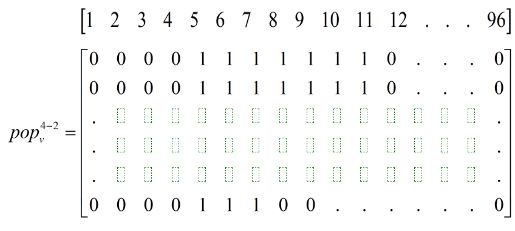
of homes (while improving their comfort) by smartly dispatching loads during periods of low electricity cost [5].
The overall grid operation thus aims at optimally scheduling generation and load dispatch to ensure that there
is a balance betwen demand and supply while meeting the individual objectives of SSEMS, TLMS and HEMS.
Integrated energy systems (IES) promote the concept of a synergized and harmonized community of energy
systems based on the bi-directional flow of information (data). This synergy in terms of operation and infor-
mation flow improves system’s efficiency [25]. The concept of IES is however at variance with the traditional
electricity grid operation which isolates the individual operations of each management system. In creating a
synergy of operations, IES also provide a platform for the exploitation of such concepts as demand side man-
agement (DSM) through price based demand response (DR) and direct load control (DLC). These initiatives
become very important considering spiralling energy demand and the huge costs involved in power plant capac-
ity expansion. For example, the energy crisis of South Africa which started in 2008 led to serious load shedding
and blackouts across the country affecting homes and businesses [30, 33]. Depleted reserve margins due to
long years of non-investment in building additional power plants to cater for growing electricity demand was
blamed for the crisis. However, the huge costs involved in building power plants and the long time frame from
conceptualization to eventual completion and synchronization of the power plant output with the grid [39] have
seen power shortages, loadshedding and grid interruptions extending to 2015 [33]. Furthermore, the growing
population and increasing industrial activities [50] mean that other alternatives besides increasing generation
capacity be exploited to guarantee electricity availability and security.
A review of existing government policy via its Integrated Resource Plan (IRP) [14] shows no significant
improvement in existing DSM capacity in the short to medium term. In the same vein, Eskom’s participation in
the DSM sector is centred around efficiency initiatives such as distribution of energy efficient compact fluorescent
lamp (CFL) bulbs [15] with moderate investments in solar water heating [21], wind [20], concentrating solar
power (CSP) [16] etc. According to [23, 22], Eskom plans to start decommissioning ageing power plants
(Camden, Hendrina and Arnot) from 2021. While it is envisaged that ongoing construction works on Medupi,
Kusile, Dedisa and Ingula power plants together with new coal independent power projects (IPP) would deliver
an additional 8249 MW to the grid between 2017-2020 as shown in Table 1, the issue of delays due to technical
constraints [17] cast huge doubts over Eskom’s proposed commissioning plans. The need therefore arises for
alternatives that will mitigate greatly the problems of blackouts and grid failures owing to demand exceeding
supply.
Demand side management (DSM) techniques have been investigated and proven to be viable alternatives to
regulating the consumption of electricity from the consumer side with applications from residential to industrial
sectors [1, 34, 27, 29, 8, 2]. According to [46], the two techniques for DSM from the consumer side include energy
efficiency improvement programs (insulation, sealing, solar water heating systems etc.) and demand response
(DR) programs (price based and incentive based). While the energy efficiency improvement programs aim at
increasing efficiency by reducing the amount of electricity required to accomplish similar tasks (with absence
of supply side interference), the DR programs are initiated primarily by the supplier to influence consumer
demand patterns. The home energy management systems (HEMS) [35, 45, 43, 26, 49, 7] are the backbone of
DR program initiatives as they provide the platform for home owners to interact with their electrical appliances
and their meters [42]. On the supply side, its management system (SSEMS) refers to actions taken to ensure that
electricity is generated and supplied at lowered operating costs, reduced environmental emissions and optimal
system reliability [28].
A review of available literature with particular focus on South Africa’s electricity sector reveals that the
operations of the HEMS and SSEMS have been largely independent of each other. In attempting to extend the
focus area outside of South Africa, [28] argued on the need for the integration of HEMS (DSM) and SSEMS for
a realistic power system planning. The need therefore exists for a platform that is capable of harmonizing the
constraints of both the supply side and demand side with the aim of:
Reducing consumer electricity bill through the application of dynamic pricing - HEMS objective
Mitigating energy poverty by extending the usage of owned electrical appliances through reduced electricity
bills. This is necessary since energy poverty is not only a function of ownership of electrical appliances
but duration of use.
Reducing operations and emissions cost of the supply side - SSEMS objective.
In doing so, the proposed platform must be capable of optimally scheduling DR loads (consumer controlled
or utility controlled) in a DSM window (from generating capacity). This research work therefore contributes to
existing DSM initiatives by:
(1) Extending the ongoing discussions on DSM initiatives by highlighting the need for synergy between
HEMS and SSEMS and its benefits.
(2) Modelling and designing a centralized energy management system (CEMS) that accepts constraints and
requirements from both the consumers and suppliers and optimally schedules DR loads for dispatch to meet
the individual constraints.
2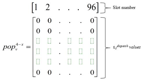
Table 1: 2017-2020 Planned Power Plant Capacity Increment [22]
                                          Medupi         Kusile      Ingula             New coal              O & C CGT
    Year                                Unit MW Unit MW Unit MW Unit                      Name      MW    Unit Name MW
    2017                                  3     738    2      738   4     333
                                          4     738
    2018                                  5     738    3      738

3
                                                       3      738
    2019                                  6     738    5      738                 1     Coal IPP1   200    3   Dedisa   237
                                                                                  2     Coal IPP1   200
    2020                                               6      738                 1     Coal IPP3   200    4   Dedisa   237
                                                                                  2     Coal IPP3   200
    IPP -   Independent Power Producer
(3) Optimally scheduling a DSM window from the generating plant overall capacity within which DSM loads
can be dispatched. The DSM window is a fraction of the power plant overall capacity within which DR loads
are to be dispatched based on the user requirements (time flexibility in dispatching load).
In attempting to model and design the proposed CEMS, one hundred thousand random homes in South
Africa within the Limpopo province are selected. Furthermore, three deferrable loads (washing machine, cloth
dryer and dish washer) are selected per house with 3 possible time-dispatch classes. Home owners are lastly
provided with a control to select the time-window (2 hours, 6 hours or 24 hours) within which dispatch of
participating DDSM loads should be done. Dynamic pricing (DP) is used along with time of use (TOU) pricing
for comparison. The power plant utilized in carrying out the dispatch of the participating DR loads is the
Medupi power plant which has been modelled to utilize carbon capture and sequestration (CCS) technology.
The dispatch of the participating DSM loads is done using a standard deviation biased genetic algorithm
(SDBGA).
The rest of the paper is organized as follows. Section 2 presents a review of related works and a justification
for this research; Section 3 presents the case study description while CEMS is briefly modelled in Section 4. The
mathematical description of the problem, pricing method adopted and SDBGA is described in Section 5. The
results obtained are discussed in Section 6 while policy implications of CEMS on the consumer and supplier
are briefly presented in Section 7. The work is concluded in Section 8 while Section 9 presents the general
applicability of CEMS.
2 Related works
An economic model for demand response with the objective of maximizing the customer utility with constraints
by either the daily budget or daily consumption was developed by [36]. The economic model was designed
to explain the consumer consumption change pattern. An energy management system (EMS) that targeted
average income earners in sub-Saharan Africa (SSA) was developed by [41]. The proposed EMS was capable
of maximizing available capacity of a residential solar based inverter by optimally scheduling competing loads.
The rule set involved in the proposed EMS did not aim at maximizing user satisfaction. In advancing the EMS
design proposed by [41], [40] proposed an EMS that was capable of controlling residential loads, maximizing
user satisfaction and minimizing household electricity cost. The lack of ’smartness’ in pre-paid meters (common
in SSA), was addressed by [42], where a smart energy management system that acted as an interface between
the meter and the consumer loads was proposed. A demand side distributed and secured energy commitment
framework and operations for a power producer in a deregulated environment was proposed by [9] while [1]
proposed a stochastic programming model using a multi-objective particle swarm optimization method for
optimizing smart grid performance, minimizing operations costs and reducing emissions with renewable sources.
Further application of DSM was done by [47] for a cement plant with a 4.2% reduction in electricity cost and
[29] for cost minimization of a water supply system. A comprehensive review on demand side tools was done by
[46] while the challenges of integrating HEMS with residential demand-side aggregators was addressed by [10].
An exploration of available literature was carried out by [3] and incentive-based DR programs were considered
to be the most suitable solutions to addressing the problem of growing per capita electricity consumption in
Kuwait. For further reading on DSM and its applications, see [4, 31, 48, 6]. The contributions of preceding works
notwithstanding, they have not been able to show the effect of DSM load control scheme (direct load control,
(DLC) or consumer control) and dispatch window on energy poverty mitigation and DSM window minimization.
This work extends research on DSM load dispatch by studying the effect of variable load control schemes (direct
load control, (DLC) and consumer control) and dispatch window (duration within which participating DSM
loads must be dispatched and completed) on the DSM load profile (DSM window minimization) and on energy
poverty mitigation.
2.1 Research motivation
A justification for this research stems from the following:
There has been a steady decline in electricity per capita for South African homes despite increasing
generation (see [37]).
Planned supply capacity expansion between 2017-2014 is over 5 times capacity loss and demand increase
within the same period. According to [22], while 3516 MW is expected to be lost due to the decom-
missioning of ageing plants between 2021 and 2024, over 19000 MW is expected to be added to the grid
generation capacity between 2017 and 2024. This translates to a net increase of about 15484 MW. The
expected addition to the grid capacity between 2017 and 2024 is over 5 times the capacity to be lost.
Demand increase within 2017 and 2024 using the high (less energy intensive) forecast from [13] is about
455078 GWh. Assuming a 70% utilization (of net increase) at 35% availability, this translates to a net
production of about 131106 GWh between 2017 and 2024.
Most of the homes in South Africa (based on [37]) are energy poor due to low electricity per capita that
prevents extended usage of owned electrical appliances.
According to [11], over 40% of global energy consumption comes from the residential and building sectors.
This thus implies that households offer great potentials for DSM initiatives.
The computation of the electricity per capita (to show declining electricity consumption) for the nine
provinces in South Africa on yearly (kWh/capita), monthly (kWh/capita), daily (kWh/capita) and hourly
(Wh/capita) basis for 2007, 2011 and 2016 is shown in [37].
3 Case study description
3.1 Consumer side problem description
One hundred thousand residential homes are selected (for the simulation) across the Limpopo province, which
is home to the Medupi power plant. Each selected home, i, is expected to possess at least a cloth washer, a
cloth dryer and a dish washer. Each selected residential home is fitted with a HEMS and allows the home owner
to:
(1) Select a class (ki ). A class corresponds to a pre-defined dispatch period for the participating DSM loads
(cloth washer, cloth dryer and dish washer). Table 2 provides further information regarding the dispatch time
and slot for each class. Three classes are offered in this modelling exercise. Thus for example, a class one choice
by house 1000 (i.e. k1 000 = 1) corresponds to 75 minutes (5 slots) duration for the cloth washer, 105 minutes
(7 slots) duration for the cloth dryer and 105 minutes (7 slots) duration for the dish washer. A slot is equivalent
to 15 minutes duration.
(2) Initialize start time (tstart
i,j ) for each appliance j. A start time need not necessarily be the eventual
dispatch time (tdispatch
i,j ).
(3) Select a dispatch window wi . A dispatch window is a period from the initialized start time (tstart
i,j ) within
which the dispatch of a participating DSM load must be completed. Thus a dispatch window selection of 1
by house 1000 (w1000 = 1) means that the window within which a DSM load selected must be dispatched and
dispatch completed is between tstart i,j and tstart
i,j + 2(8 slots).
3.1.1 Justification for choice of Limpopo Province
A justification for the choice of the Limpopo province stems from the fact that hourly electricity consumed per
person (capita) as observed from [37] as at 2016 was about 107.38W h which was among the lowest across the
provinces. CEMS application is thus necessary to investigate its potential benefit in mitigating energy poverty
among energy poor homes.
Table 2: Class description, its dispatch time and number of slots
Class Cloth washer Cloth dryer Dish washer
1 mins 75 105 105
slots 5 7 7
2 mins 60 75 75
slots 4 5 5
3 mins 30 45 60
slots 2 3 4
By definition,
1 ≤ i ≤ 100000 (1)
1≤j≤3 (2)
ki = {1, 2, 3} (3)
wi = {2, 6, 24}hours (4)
5If the daily cumulative energy demand for all DSM loads in any residential house i is Eienergy and PiF P and
PiDP are the daily fixed price cost (electricity cost using Eskom’s TOU pricing) and daily dynamic price cost
(electricity cost using dynamic pricing) of DSM loads (energy) for house i, then the HEMS aims at:
(1) Minimizing PiDP such that PiDP ≤ PiF P
(2) Optimally scheduling the dispatch time tdispatch
i,j of each appliance j for house i. Where tdispatch
i,j is the
final dispatch time of an appliance j for house i as evaluated by the SDBGA.
Thus,
tstart
i,j ≤ tdispatch
i,j + tduration
i,j ≤ tstop
i,j (5)
where tduration
i,j is the duration period for appliance j and house i as obtained from Table 2.
tstop start
i,j = ti,j + wi ∗ (6)
Thus, the cost function associated with the HEMS is defined as
ZHEM S = minimize(PiDP ) (7)
Table 3 presents the power rating of the participating DSM loads for each residential house.
Table 3: Cloth washer, cloth dryer and dish washer statistics
Equipment Device Rating (W) Number per household Total Power (W)
Cloth washer 500 1 500
Cloth dryer 1000 1 1000
Dish washer 1200 1 1200
3.1.2 Justification for ki and wi pre-selection
The pre-selected dispatch times for the cloth washer (30 mins., 60 mins. and 75 mins.), cloth dryer (45 mins.,
75 mins. and 105 mins.) and dish washer (60 mins., 75 mins. and 105 mins.) mirror conventional use time and
makes for ease in simulating their use. Also, the pre-defined windows wi are provided to offer the utility some
flexibility in dispatch. While it is expected that a house that selects wi∗ = 8 intends for tdispatch
i,j = tstart
i,j , the
dispatch start
inconvenience in ti,j > ti,j is expected to be compensated by reduced electricity bills.
3.2 Supply side problem description
In dispatching the participating loads, the Medupi power plant is modelled to utilize carbon capture and
sequestration (CCS) technology. From the consumer side, two kinds of loads are easily deduced - base/bulk
load and the DSM load. A DSM window is to be created within the operating profile of the power plant within
which loads participating in DSM would be dispatched. Furthermore, dispatch of residential loads is to be done
to ensure optimal power plant utilization and reduced operations costs. The SSEMS thus aims at:
(1) Minimizing the DSM window C DSM in the power plant operations profile within which the DSM loads
can be dispatched. This leads to maximization of the base load capacity C BL .
(2) Maximizing the utilization of the power plant capacity U util .
(3) Minimizing the power plant operations cost F OP cost .
(4) Minimizing the power plant emissions cost F Ecost .
(5) Maximizing earnings PiDP from each household.
The relationship between the power plants reserve capacity (C Reserve ), base load capacity (C BL ) and DSM
capacity (C DSM ) is shown in equation (8) while the operations cost of the power plant is computed as shown
in equation (9).
C BL + C DSM + C Reserve = C P lant (8)
F OP cost = a + (b × εt ) (9)
t
where a and b are gotten from Table 4, ε is the loading factor (i.e. the fraction) of the power plant currently
being utilized and t is the slot being considered. In a 24-hour modelling window with 15 minutes interval, there
are four slots per hour. This translates to 96 slots for 24 hours.
Assuming ZSSEM S to be the cost function associated with the supply side, then its description is shown
subsequently.
ZSSEM S = max(P DP , U util ) + min(F OP cost , F Ecost , C DSM ) (10)
6Table 4: Modified Medupi Power Plant Modelling Parameters
LCOE model values Operating range (%) Carbon emissions Capacity
Technology a b min max norm (kg/MWh) (MW)
CCS 2815.21 -14.80 66 88 85 136.2 1588
LCOE - Levelized cost of energy
CCS - Carbon capture and sequestration
Operating range - capacity factor range for the power plant
3.2.1 Normalization of SSEMS associated parameters
ZSSEM S is a non-linear function and cannot be resolved using exact solutions since its optimization cuts across
parameters that are of varying units. For example, while P DP , F Ecost and F OP cost are in ZAR, U util is
expressed as a percentage (%) while C DSM is in M W . To resolve ZSSEM S therefore, all associated parameters
are normalized. Table 5 presents the base values used in normalizing P DP , F Ecost , F OP cost , C DSM and U util .
DP Ecost OP cost DSM util
Thus, if Pnorm , Fnorm , Fnorm , Cnorm and Unorm are the normalized values for P DP , F Ecost , F OP cost , C DSM
P DP F Ecost OP cost
C DSM U util
and U , then Pnorm = P DP , Fnorm = F Ecost , Fnorm = F
util DP Ecost OP cost
F OP cost
DSM
, Cnorm =C util
DSM and Unorm = U util .
base base base base base
3.3 DSM load dispatch options
In dispatching the participating DSM loads (cloth washer, cloth dryer and dishwasher) for the 100000 houses
in the Limpopo province, two dispatch options are modelled as follows:
3.3.1 Dispatch option 1
For dispatch option 1, the customers i are in charge of selecting ki , wi and their intended start time (tstart i,j )
dispatch
for each DSM j load. In this option, the utility (Eskom) is only able to influence final dispatch time (ti,j )
dispatch 0 option1
of the load j such that tstart
i,j ≤ ti,j ≤ ti,j . The flexibility of the dispatch time denoted as f i,j | start
ti,j is
defined as:
0
Option1 ti,j − tstart
i,j
fi,j |tstart = (11)
i,j
tstart
i,j
0 0
However, ti,j = tstop duration
i,j − ti,j and tstop start
i,j = ti,j + 4wi ∗, ⇒ ti,j = tstart
i,j + 4wi ∗ −tduration
i,j Hence,
Option1 4wi ∗ −tduration
i,j
fi,j |tstart = (12)
i,j
tstart
i,j
The end limits (minimum and maximum) possible selection of wi are 2 hours (8 slots) and 24 hours (96
slots) respectively.
Option1 8−tduration
i,j Option1 96−tduration
i,j
If wi ∗ = 8, then fi,j |tstart
i,j
= tstart
and if wi ∗ = 96, then fi,j |tstart
i,j
= tstart
.
i,j i,j
Option1
The constraint on fi,j is given as:
8 − tduration
i,j Option1 96 − tduration
i,j
start ≤ fi,j |tstart ≤ (13)
ti,j i,j
tstart
i,j
Option1 96−8 88
With the operating range of fi,j |tstart
i,j
given as tstart
= tstart
i,j i,j
Option1
The computation of fi,j |tstart
i,j
is to provide an insight into how much choice the proposed standard
deviation biased genetic algorithm (SDBGA) has in optimally selecting tdispatch
i,j under the simulated options.
3.3.2 Dispatch option 2
In this option, the choice of selection of tdisptch
i,j is entirely under the control of the utility, i.e. the participating
DSM loads are under direct load control (DLC). Hence, under dispatch Option 2, wi = 3 i.e. wi ∗ = 96. However,
the consumer selects ki . By definition, under this option, tstarti,j = 1, tstop i
i,j = 96 and ti,j = 96 − ti,j
duration
.
Option2 duration Option2 duration
⇒ fi,j |tstart
i,j
= 4w i ∗ −t i,j . Thus, the operating range of f i,j | start
ti,j is 96 − ti,j . Figure 1
0
presents the time-line progression of the various time instances (tstart i, j, ti,j , tfi,jinal , tduration
i,j and tstop
i,j ).
73.4 Justification for C DSM window
As posited by [28], the integration of DSM and SSEMS is necessary for realistic system planning. Pre-selecting
the DSM window C DSM within which the participating DSM loads are to be dispatched provides the utility with
advanced information for optimal system operation. Furthermore, the utility in pre-selecting a dispatch window
C DSM is able to evaluate ahead of time, the optimal generation scheduling configuration of its generators
that will achieve its objectives in terms of reduced F Ecost and F OP cost and prevent over-sizing of spinning
reserves. However, in scheduling C DSM , great care is taken not to under-size the window to prevent utilizing
the generators beyond their normal operating range.
Figure 1: A typical time progression and execution window for DSM loads.
4 CEMS modelling
The complexity presented by the multi-objective and multi-dimensional problem is depicted in Figure 2 where
the links and connections between the proposed CEMS, HEMS and SSEMS are properly shown. Furthermore,
the ensuing conflicts that may arise from the individual objectives of HEMS and SSEMS are seen. For example,
while HEMS aims to minimize PiDP , SSEMS aims at maximizing PiDP . The resolution of this resulting conflict
is explained subsequently.
4.1 HEMS and SSEMS conflict matrix
The harmonization of the household and supply requirements does reveal some conflicts. The conflict matrix
shown in Table 6 presents the five major conflict spots between the HEMS and SSEMS working requirements.
For example, conflict C1,2 which is the conflict between the SSEMS constraint 1 and HEMS constraint 2 shows
that in trying to minimize C DSM by the SSEMS, the possibility of failing to dispatch household loads within
their pre-determined window by the HEMS is possible due to reduced C DSM . Also, conflict C2,2 describes the
possibility of low utilization of power plant capacity by the SSEMS due to low dispatch of residential DSM
loads within certain periods owing to external constraints like line ampacity limits. The conflict C4,1 denotes
the conflict that arises in trying to reduce emissions cost by the SSEMS. The unintended consequence might be
a higher cost of electricity P DP for households during such periods. Similarly, conflict C4,2 arises when SSEMS
in trying to reduce F Ecost selects tdispatch
i,j under dispatch option 1 that is outside the range (tstart start
i,j , ti,j + wi ).
DP
Conflict C5,1 denotes a direct conflict between SSEMS and HEMS in optimizing Pi . While SSEMS strives
at maximizing its value, HEMS aims at minimizing it. A platform is thus needed that is capable of addressing
these constraints and optimally scheduling tdispatch
i,j of consumer DSM loads within the HEMS and SSEMS
defined limits.
8Figure 2: Proposed CEMS infrastructure incorporating the HEMS and SSEMS.
5 Mathematical modelling
This section presents the mathematical description for HEMS, SSEMS and SDBGA including discussions on
the pricing models adopted and power plant utilized and their justification.
5.1 HEMS constraints modelling and description
Three classes ki as shown in Table 2 and equation (3) are adopted in this research. A selection k100 = 2 implies
that class 2 has been selected by house 100. A consequence of this thus implies that the dispatch time of the
washing machine, cloth dryer and dish washer is 75 minutes (5 slots), 105 minutes (7 slots) and 105 minutes (7
slots) respectively. An initial start time tstart
i,j and dispatch window wi is selected by the user for every appliance
(under dispatch option 1).
dispatch
Given tstart
i,j , ki and wi , a dispatch time ti,j is sought such that
0
tstart
i,j ≤ tdispatch
i,j ≤ ti,j (14)
0
where ti,j is the final time a DSM device j for house i must be dispatched to meet with the user pre-
determined window wi selection. By dispatch, we mean ”turned on.”
Thus, 0
ti,j = tstop duration
i,j − ti,j (15)
The associated cost of dispatch which is evaluated using both the time of use (TOU) pricing and dynamic
pricing (DP) for comparison purposes is computed as follows: Let F P t be the TOU price and DP t the dynamic
price, then X energy
PiDP = (DP t ∗ Ei,j,t ), t = tdispatch
i,j : tfi,jinal , i = 1 : 100000, j = 1 : 3 (16)
X energy
PiF P = (F P t ∗ Ei,j,t ), t = tdispatch
i,j : tfi,jinal , i = 1 : 100000, j = 1 : 3 (17)
95.2 SSEMS constraints modelling and description
Figure 3 presents the typical profile of the Medupi power plant showing the base load (C BL ), DSM (C DSM )
and reserve allocations (C Reserve ). Assuming a maximum operating range (capacity factor) of 88% (as obtained
from Table 4), the following is obtained:
C DSM + C BL = 1397.44M W (18)
C Reserve = 190.56M W (19)
util
The utilization cost U is applied to utilization of the Medupi power plant capacity below 70% for any
time t. This is necessary to prevent the build-up of peaks unnecessarily thus allowing for a evenly distributed
dispatch profile. Thus, if Ututil ≥ 70%, then Ututil = 0, else Ututil = utilcost (t).
96
X
U util = Ututil (20)
t=1
The emissions cost F Ecost is computed based on the CO2 emissions equivalent (kgCO2 ) for energy (electric-
ity) produced and consumed (MWh). Thus,
96
X X
F Ecost = (Emit × (Etenergy ) × b1 × b2 ) (21)
t=1 i,j
where b1 is the conversion factor to ZAR and b2 is the conversion factor of Etenergy from M W to M W h. F Ecost
is computed as shown in [32]. To convert to ZAR, prevailing exchange rate from [44] was used. SSEMS thus
seeks to achieve an optimum operating point on its constraint wheel as shown in Figure 4 that guarantees load
dispatch at minimum costs (environment, operations) and maximized income and generator utilization. Figure
4 presents the normalized constraint wheel for the SSEMS with each normalized factor having a range of possible
selection. SSEMS thus selects points for each normalized factor that gives it the best operating conditions.
Figure 3: A typical capacity profile of the Medupi power plant.
10Figure 4: SSEMS constraint wheel.
5.3 Price modelling
Two pricing schemes have been adopted for this model and they are the exiting Eskom TOU pricing scheme
and a dynamic pricing scheme.
5.3.1 Time of use pricing
The existing TOU pricing scheme assumes a flat rate price of 1.25/kW h for off-peak periods with a 20%
increment during 6am - 8am and 6pm - 8pm. The selected Eskom TOU pricing scheme is for a household whose
monthly electricity consumption is less than 600kW h. Weekends and weekdays have been assumed to have the
same profile. The sample TOU dispatch profile for a day is shown in Figure 5.
5.3.2 Dynamic pricing
The computation of the dynamic price DP t follows the time of use (TOU) pricing being used by Eskom. As
seen in Figure 5, the daily average dynamic price is equivalent to Eskom’s TOU pricing (excluding the peak
1
Pt=24
periods). Given F P t as the real time TOU pricing electricity spot price, then 24 t t
t=1 (DP ) = F P .
5.4 Motivation for dynamic pricing model selected
The TOU pricing scheme is adopted by Eskom to shift demand from peak periods to off-peak periods in order to
prevent system collapse due to demand exceeding supply. In doing so, peak demand reduction is a motivation.
However, the proposed dynamic pricing aims at:
Improving the flexibility of the grid by offering the utility greater control of the electricity network. This
is mostly the aim of dispatch option 2 in which the participating DSM loads are under DLC by the utility.
Reducing electricity bills of consumers. The adoption of real time pricing guarantees the home-owners a
reduction in their electricity bills over TOU pricing without altering their comfort level. In doing this,
home-owners are able to save money that could be used in extending usage of electrical appliances.
Reducing grid expansion investments. With the adoption of dynamic pricing and the subsequent control
the utility has over the dispatch of participating DSM loads, the over-sizing of spinning reserves would be
reduced since the utility can almost adequately predict the behaviour of the grid and optimize its overall
operations.
11Figure 5: TOU pricing and dynamic pricing profiles.
5.5 SDBGA modelling
The proposed genetic algorithm (SDBGA) is a variant of MMIGA used in [42]. In differing from MMIGA,
SDBGA computes the standard deviation of a generation matrix and selects the population with the highest
spread. The notion behind this idea is to select the allocation that offers more spread in allocation of DSM
loads dispatch time. This is to prevent the build up of multiple peaks.
5.5.1 Population initialization
pop1v for start times, pop2v for class selection, pop3v for window selection and pop4v for final dispatch time are
generated as follows:
pop1v = {tstart start start start start start start start start start start start
1,1 , t1,2 , t1,3 , t2,1 , t2,2 , t2,3 , t3,1 , t3,2 , t3,3 , ..., t100000,1 , t100000,2 , t100000,3 } (22)
pop2v = {k1 , k2 , k3 , k4 , ..., k100000 } (23)
pop3v = {w1∗ , w2∗ , w3∗ , w4∗ , ..., w100000
∗
} (24)
pop4v = {tdispatch
1,1 , tdispatch
1,2 , tdispatch
1,3 , tdispatch
2,1 , tdispatch
2,2 , tdispatch
2,3 , tdispatch
3,1 , tdispatch
3,2 , tdispatch
3,3 , ..., tdispatch dispatch dispatch
100000,1 , t100000,2 , t100000,3 }
(25)
∗
The selection of tstarti,j and w i is either by the consumer (dispatch option 1) or the utility (dispatch option
2) while ki selection is solely by the consumer. This then implies that η(pop1v ) = η(pop4v ) = 300000 and
η(pop2v ) = η(pop3v ) = 100000. Furthermore, tfi,jinal = tstart i,j + wi∗ − 1 (for dispatch option 1) and tfi,jinal = 96 (for
dispatch option 2). The incorporation of −1 is to compensate for start position and prevent over-float. Three
population matrices (pop4−x v , x = {1, 2, 3}) with dimensions dim1 × dim2 (dim1 = number of rows ornumber
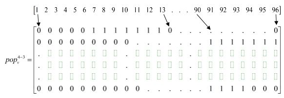
of houses and dim2 = number of slots) are also initialized to zero as shown in Figure 6. pop4−x v represents
the matrix for tdispatch
i,j such that pop 4−1
v collects tdispatch
i,1 values, pop 4−2
v collects t dispatch
i,2 values while pop4−3
v
dispatch
collects ti,3 values.
12Figure 6: pop4−x
v initialization description.
5.5.2 pop4−x
v filling
The filling of pop4−x
v is done based on the tdispatch
i,j stochastically evaluated for each household such that tstart
i,j ≤
dispatch 0
ti,j ≤ ti,j . Let popv = {2, 5, 5, 1, 1, 1, ..., 3, 3, 88}, pop2v = {1, 1, ..., 3} and pop3v = {8, 96, ..., 8} be the
1
associated statistics for houses 1, 2 and 100000. This implies that houses 1 and 100000 are under the dispatch
option 1 while house 2 is under the dispatch option 2. The description for the houses is as follows:
f inal
House 1: tstart duration
1,1/2/3 = {2, 5, 5}, t1,1/2/3 = {5, 7, 7} while t1,1/2/3 = {9, 12, 12}. All values are in slots. The
range of the dispatch value for the DSM loads j for house 1 is given to be {2, 5, 5} ≤ {tdispatch
1,1 , tdispatch
1,2 , tdispatch
1,3 }≤
dispatch dispatch dispatch
{5, 6, 6}. The implication of this is that 2 ≤ t1,1 ≤ 5, 5 ≤ t1,2 ≤ 6 and 5 ≤ t1,3 ≤ 6.
f inal
House 2: tstart duration
2,1/2/3 = {1, 1, 1}, t2,1/2/3 = {5, 7, 7} while t2,1/2/3 = {96, 96, 96}. All values are in slots. The
range of the dispatch value for the DSM loads j for house 2 is given to be {1, 1, 1} ≤ {tdispatch
2,1 , tdispatch
2,2 , tdispatch
2,3 }≤
dispatch dispatch dispatch
{92, 90, 90}. The implication of this is that 1 ≤ t2,1 ≤ 92, 1 ≤ t2,2 ≤ 90 and 1 ≤ t2,3 ≤ 90.
f inal
House 100000: tstart duration
100000,1/2/3 = {3, 3, 88}, t100000,1/2/3 = {2, 3, 4} while t100000,1/2/3 = {10, 10, 95}. All
values are in slots. The range of the dispatch value for the DSM loads j for house 100000 is given to be
{3, 3, 88} ≤ {tdispatch dispatch dispatch dispatch
100000,1 , t100000,2 , t100000,3 } ≤ {9, 9, 92}. The implication of this is that 3 ≤ t100000,1 ≤ 9,
dispatch dispatch
3 ≤ t100000,2 ≤ 9 and 88 ≤ t100000,3 ≤ 92.
In filling pop4−x
v , SDBGA aims at varying tdispatch
i,j within its minimum (tdispatch
i,j ) and maximum (tdispatch
i,j )
limits to ahieve the objectives of HEMS and SSEMS.
5.5.3 pop4−x
v initialization
An initial allocation of tdispatch
i,j is made for all houses i and load j in pop4−x
v . The values randomly generated
0 0
for tdispatch
i,j are always constrained by tstart
i,j ≤ tdispatch
i,j ≤ ti,j (tdispatch
i,j = tstart
i,j and tdispatch
i,j = ti,j ) . In filling
pop4−x
v with tdispatch
i,j values, the range {tdispatch i, j, tdispatch
i,j + tduration
i,j − 1} is initialized to 1. Figures 7, 8 and
4−x
9 present the initialization of popv for houses 1, 2 and 100000. It is observed from Figure 7 that for house 1
in pop4−1
v , slots 3 − 7 are initialized to 1, similarly, for house 2 in pop4−1v , slots 60 − 64 are initialized to 1 while
for house 100000 in pop4−1v , slots 4 − 5 are initialized to 1. The same rule is used in filling pop4−2
v and pop4−3
v
based on each house’s description given in section 5.5.2.
Figure 7: pop4−1
v filling.
135.5.4 tdispatch
i,j variation
For each filling of pop4−x v
4−x
, Epower is computed. Ev4−x is the cumulative column sum of power in pop4−x v .
4−x 4−x
In generating Epower , popv is multiplied by its respective power value. From Table 3, x = 1 −→ power
value is 500W . Similarly, x = 2 −→ P power value is 1000W while x = 3 −→ power value is 1200W . Thus,
96
Ev4−x = {ex1 , ex2 , ..., ex96 } where exu = 4−x
u=1 popv
4−x
(1 : 100000, u). The generation of Epower enables us to
identify peak points and under-utilization points. These points are then isolated and used in varying tdispatch
i,j .
However, in the event that the constraints placed on tdispatch i,j prevent it from being dispatched to points of
under-utilization, then it is randomly computed using its constraints - tdispatch
i,j for minimum and tdispatch
i,j for
maximum to be round(randi×(tdispatch
i,j tdispatch
i,j )+tdispatch
i,j ) where round is a function that converts any floating
value to the nearest integer and 0 < randi < 1.
Figure 8: pop4−2
v filling.
Figure 9: pop4−3
v filling.
5.5.5 Cost computation and optimal solution selection
For each run of pop4−x
v , PiDP , PiF P , F OP cost , F Ecost , U util , C DSM and standard deviation (sdv ) is computed.
Furthermore, the cost, Zv associated with each population is calculated and used in ranking each solution.
optimum
Selection of optimum solution, Sgen is done as follows:
4−x 4−x
Given any pop1 and pop2 as the best population matrices per generation, gen, with standard deviations,
sd1 and sd2 , if |Z1 − Z2 | ≤ 1% of |Z1 + Z2 | and sd1 < sd2 , then Sgen optimum
= pop4−x
1
optimum
else Sgen =
4−x
pop2 .
5.6 Medupi Power plant
The Medupi power plant is a greenfield coal fired power plant project situated in the Limpopo province. On
completion, it is expected to be the fourth largest coal plant in the world. It has an installed capacity of 4764
MW from its six units each capable of outputting 794 MW. Unit 6 (the first of the 6 units) was synchronized
with the grid in 2015. It has a planned operational lifetime of about 50 years [19, 18]. In evaluating statistics
such as loading factor, operations cost, environmental costs (εt , F OP cost , F Ecost ) etc., there was the need to
be able to characterize the behaviour of the Medupi power plant under varying loading conditions. A modified
artificial neural network MANN [38] was applied on data plot describing the evolution of the levelized cost of
energy for various power plants [14] to generate constants a and b as shown in Table 4. The choice and use of
the Medupi power plant is because of its proximity to the customers being considered. Furthermore, its capacity
is capable of dispatching the baseload and DSM loads of the considered consumers hence its choice.
146 Results and discussion
In modelling the allocation of consumer loads based on their selected and optimized parameters (dispatch
option 1), a controlled allocation (dispatch option 2) was also done to provide a basis for comparison and
standardization. The controlled allocation (dispatch option 2) assumes wi = 3 (i.e. the utility selects the start
time of participating DSM loads) for all customers with all other selections remaining the same (under the user’s
control). Table 7 presents the distribution of households across the various classes under both dispatch options
(1 and 2) while Table 8 presents the distribution of houses across the various dispatch windows.
Table 9 presents the values of associated parameters for both dispatch options (1 and 2). It is observed
from Table 9 that dispatch option 2 achieves a better minimization of C DSM of 14.94M W compared to a peak
C DSM of 40.77M W for dispatch option 1. In terms of plant utilization (U util ), dispatch option 2 also produces
a better value of 87.92% compared to 86.30% by dispatch option 1. The operations cost (F OP cost ) is higher for
dispatch option 1 compared to dispatch option 2 while dispatch option 1 is more environmentally friendly with
F Ecost of ZAR 11,288,439 compared to ZAR 11,501,166 by dispatch option 2. Dispatch option 1 was also found
to be more consumer friendly from Table 10 under dynamic pricing with a total cumulative cost for the DSM
loads (P DP ) of ZAR 373,218.40 to the residential houses. This is in contrast to a (P DP ) of ZAR 416,280.20
from dispatch option 2. However, dispatch option 2 provided a better fixed price cost (P F P ) of ZAR 433,185.30
compared to dispatch option 1’s fixed price cost of ZAR 438,153.40.
The area plots shown in Figures 10 and 11 depict the cumulative load profile (base load, cloth washer, cloth
dryer and dish washer) for both dispatch options (1 and 2) respectively. The computation of the actual cloth
washer value is done by deducting the read out cloth washer value from the plot and deducting the base value
from it. Also, the computation of the cloth dryer value is done by deducting from the read out cloth dryer plot
value the cumulative sum of the base load value and the corresponding cloth washer value. The actual dish
washer value is computed by deducting from the dish washer plot value the cumulative sum of the base load
value and the corresponding cloth washer and cloth dryer values. It is observed from Figure 10 that its profile
is influenced greatly by the dynamic pricing curve. With over 50% of households selecting class 2, the utility
is given more leverage to shift dispatch time of DSM loads away from the early hours of the day to periods of
low prices. However, for selections that must be done within the periods of high cost, the utility is forced to
optimally schedule the DSM loads to be dispatched at periods with lower costs. This is however done within
the limits allowed by the other prevailing constraining parameters (F Ecost , F OP cost etc.). Figure 11 however
presents a profile which is evenly distributed across the day irrespective of the dynamic pricing profile. This
explains why the P DP for dispatch option 2 is higher than that for dispatch option 1 as shown in Table 9.
Figure 10: Option 1 cumulative power profile.
15Figure 11: Option 2 cumulative power profile.
In evaluating the actual expenditure and potential savings (if any) for both options, the associated energy
(Eienergy ), dynamic pricing cost (PiDP ) and fixed price cost (PiF P ) for selected houses for both dispatch options
1 and 2 are shown in Table 10. It is important to point out that the costs shown in the Table 10 are primarily
for the DSM loads under consideration (cloth washer, cloth dryer and dish washer) and are independent of
standing charges and other associated costs. From Table 10, it is noticed that dispatch option 1 achieves daily
savings of 6.5%, 19.7%, 39.2%, 44%, 31.7% and 29.5% for houses 1, 1000, 10000, 25000, 33000 and 71000.
Furthermore, a higher dynamic cost is observed for the house 7 under dispatch option 1 out of the ten houses
under consideration. However, dispatch option 2 has more houses (4) compared to dispatch option 1 (1) incurring
higher electricity cost using dynamic pricing for the houses under consideration.
Table 11 presents the disparity in dispatch time (tdispatch
i,j ) for each DSM appliance under both dispatch
options (1 and 2) for the houses under consideration. The variation in the dispatch time evaluated for both
dispatch options (1 and 2) is further depicted in Figure 12, which presents the dispatch (power) of the three DSM
appliances for house 1 for both dispatch options (1 and 2). House 1 dispatch of participating DSM loads (cloth
washer, cloth dryer and dish washer) under both dispatch options (1 and 2) results in tdispatch
option1/option2 = {59, 25}
for cloth washer, tdispatch dispatch
option1/option2 = {85, 34} for cloth dryer and toption1/option2 = {42, 92} for dish washer. The
computation of the standard deviation for the dispatch values gives 17.68 for dispatch option 1 and 30 for
dispatch option 2 which implies that the utility achieves a better spread of the dispatch times and also achieves
a 23.8% savings (for dispatch option 2) compared to a 6.46% savings (for dispatch option 1).
7 Policy discussion on results
As earlier highlighted among the HEMS and SSEMS objectives, electricity cost reduction and greater system
flexibility are some overaching reasons for proposing the integration of SSEMS and HEMS. Considering the
implications of [37] which shows declining electricity per capita values and [13] where it can be argued that
planned capacity expansion might be over-sized, we present some implications of the results obtained on the
consumer and the supply side.
7.0.1 Policy implication of CEMS on consumers
Results obtained from CEMS modelling (that integrates HEMS and SSEMS constraints) show that averagely,
reduction in electricity bills of consumers is guaranteed for CEMS platform that incorporates dynamic pricing.
The introduction of dispatch windows and the incorporation of dynamic pricing mean homeowners are not forced
to avoid electricity usage during peak hours due to higher electricity prices under TOU pricing. For example,
results from Table 10 show that on average, dispatch option 1 saves each participating house 519.48W h/day
with dispatch option 2 saving 135.24W h/day.
16Table 5: Base value for all cost component elements.
Component Base value id Base value Evaluation description
DP
P DP Pbase 588000 ZAR Evaluated by computing cost of total DSM energy E energy with unit electricity price of 1.5ZAR/kW h
FP
PFP Pbase 588000 ZAR Evaluated by computing cost of total DSM energy E energy with unit electricity price of 1.5ZAR/kW h
util
17
U util Ubase 100 Assumed 100% plant capacity utilization
OP cost
F OP cost Fbase 145230 ZAR Evaluated using a and b values gotten from Table 4 and loading factor (ξ t ) of 88%
Ecost
F Ecost Fbase 11511239 ZAR Evaluated using emissions value from Table 10 and cost value from [32]. Conversion from Pounds to ZAR is done from [44]
DSM
C DSM Cbase 30 MW Selected by inspection
dispatch
tdispatch
i,j ti,j,base tstart
i,j tstart
i,j is the intended start time/reference point for tdispatch
i,jTable 6: SSEMS-HEMS conflict matrix
HEMS
1 2
1 X
2 X
SSEMS 3
4 X X
5 X
Table 7: Household class ki distribution for the various options
Class ki
Option 1 2 3
1 24887 50185 24928
2 24887 50185 24928
Table 8: Household dispatch window wi distribution for the various options
Dispatch window wi
Option 1 2 3
1 25043 50037 24920
2 0 0 100000
Table 9: Associated parameter values for the various options
Options
Parameters 1 2
BL
Baseload, C (MW) 1356.67 1382.50
Plant utilization, U util (%)∗∗ 86.30 87.92
Peak C DSM (MW) 40.77 14.94
Cumulative Energy, E energy (M W h)∗ 329.31 329.31
F OP cost (ZAR)∗∗ 147640.50 145329.80
F Ecost (ZAR)∗∗ 11288439 11501166
P DP (ZAR)∗ 373218.40 416280.20
P F P (ZAR)∗ 438153.40 433185.30
* - DSM loads only
** - DSM + baseloads
18Table 10: PiDP and PiF P for selected houses under the various options for one day
Option 1 Option 2
House number, i Eienergy (kWh) ki wi PiDP (ZAR) PiF P (ZAR) % savings PiDP (ZAR) PiF P (ZAR) % savings
1 2.2 3 2 2.57 2.75 6.46 2.14 2.81 23.8
7 3.25 2 24 4.69 4.19 -11.89 5.04 4.19 -20.25
1000 3.25 2 6 3.51 4.38 19.67 4.43 4.31 -2.69
19
10000 4.475 1 2 3.82 6.28 39.16 4.87 5.81 16.14
25000 4.475 1 2 3.53 6.31 44 3.30 6.06 45.55
33000 2.2 3 24 2.08 3.05 31.72 3.66 2.75 -33.01
45000 2.2 3 6 2.68 2.90 7.70 1.90 2.78 31.65
71000 3.25 2 24 2.95 4.19 29.46 5.17 4.06 -27.38
92000 2.2 3 6 2.57 3.05 15.73 2.14 2.81 23.90
100000 3.25 2 6 3.50 4.36 19.80 4.60 4.81 4.52The benefit of this is that homeowners could either extend usage of owned electrical appliances or direct the
savings to other activities that improve their Quality of Life (QoL).
7.0.2 Policy implication of CEMS on electricity suppliers
A major problem in electricity generation and supply is in sizing spinning reserves. Mostly, reserve margins
are oversized in anticipation of demand increase which leads to higher operations cost, environmental costs
and inefficiency. Providing the electricity supplier with some control over dispatch times of consumer loads
(participating in DSM) offers the supply side greater flexibility in optimally scheduling generation resources.
From Table 9, dispatch option 2 achieves a 1.6% reduction in operations cost over dispatch option 1 with
dispatch option 2 achieving a better operations profile as shown in Figure 11.
Table 11: tdispatch
i,j for selected houses under the various options
Cloth washer Cloth dryer Dish washer
House number, i tdispatch
Option1 tdispatch
Option2 tdispatch
Option1 tdispatch
Option2 tdispatch
Option1 tdispatch
Option2
1 59 25 85 34 42 92
7 29 29 48 52 53 9
1000 46 28 73 66 56 42
10000 76 21 60 15 72 89
25000 33 17 78 74 74 82
33000 33 14 60 9 76 38
45000 58 20 38 93 67 63
71000 71 50 5 11 87 7
92000 33 35 40 32 73 92
100000 55 19 56 69 68 28
Figure 12: Options 1 and 2 dispatch profile for house 1 DSM loads.
8 Conclusion
This research work has presented in detail the optimization of a DSM window on the Medupi power plant, for
100000 residential houses in South Africa. Using a CEMS (which incorporates a SDBGA), a synergy between
HEMS and SSEMS has been established as well as the resolution of the ensuing SSEMS-HEMS conflict matrix.
Two Options have been modelled (with dispatch option 2 acting as a control for the standardization of the
proposed model) for all residential houses and DSM loads. A critical evaluation of the two options shows that
20dispatch option 1 outperforms dispatch option 2 in minimizing F Ecost and P DP . Furthermore, dispatch option 1
has been shown to be sensitive to the dynamic pricing model adopted as it strives to shift dispatch of consumer
loads from the periods of higher costs to periods of lower costs. This is at variance with dispatch option 2
which is quite insensitive to the dynamic pricing model and strives to achieve an evenly distributed profile and
minimized DSM window at the expense of higher consumer and environmental costs. Average overall plant
capacity utilization by dispatch option 1 has also been shown to be 86.3% which competes favourably with
87.92% obtained by dispatch option 2.
This research has thus shown that handing over total control of the dispatch time of participating DSM
loads to the utility (dispatch option 2) is at variance with the aim of dynamic pricing. This is due to the reasons
deduced from Table 9 where dispatch option 2 is seen to strive for a very strict minimized DSM window with
the consequence of higher environmental costs and higher dynamic price cost due customers. This thus defeats
the incentive behind price based demand response. However, this research has shown that the variability in
consumers choice of dispatch start times and dispatch windows introduces robustness to the model and enhances
its ability to search for an optimal solution with significant benefits to both the consumers and suppliers.
In extending this research, a multi-DSM window is being exploited with varying dynamic pricing schemes
to see how well this proposed model performs under such multi-complex situation.
9 General applicability
While this work has utilized statistics relating to South Africa to test the proposed CEMS model, CEMS is
of general application. This is because the associated statistics such as DSM loads, window, class, number of
participating houses etc. are all plug-ins and do not interfere with the model description but are rather used in
optimizing the dispatch of DSM loads based on pre-determined criteria.
10 Acknowledgement
The financial assistance of the National Research Foundation (NRF) and The World Academy of Sciences
(TWAS) through the DST-NRF-TWAS doctoral fellowship towards this research is hereby acknowledged. Opin-
ions expressed and conclusions arrived at, are those of the authors and are not necessarily to be attributed to
the NRF. The authors also appreciate the anonymous reviewers for their helpful comments.
References
[1] G.R. Aghajani, H.A. Shayanfar, and H. Shayeghi. “Demand side management in a smart micro-grid in the
presence of renewable generation and demand response”. In: Energy 126 (2017), pp. 622 –637. issn: 0360-
5442. doi: https://doi.org/10.1016/j.energy.2017.03.051. url: http://www.sciencedirect.
com/science/article/pii/S0360544217304139.
[2] K. Al-jabery et al. “Demand-Side Management of Domestic Electric Water Heaters Using Approximate
Dynamic Programming”. In: IEEE Transactions on Computer-Aided Design of Integrated Circuits and
Systems 36.5 (2017), pp. 775–788. issn: 0278-0070. doi: 10.1109/TCAD.2016.2598563.
[3] Rajeev Alasseri et al. “A review on implementation strategies for demand side management (DSM) in
Kuwait through incentive-based demand response programs”. In: Renewable and Sustainable Energy Re-
views 77 (2017), pp. 617 –635. issn: 1364-0321. doi: https://doi.org/10.1016/j.rser.2017.04.023.
url: http://www.sciencedirect.com/science/article/pii/S1364032117305282.
[4] M.H. Alham et al. “Optimal operation of power system incorporating wind energy with demand side
management”. In: Ain Shams Engineering Journal 8.1 (2017), pp. 1 –7. issn: 2090-4479. doi: https:
//doi.org/10.1016/j.asej.2015.07.004. url: http://www.sciencedirect.com/science/article/
pii/S2090447915001094.
[5] S. Althaher, P. Mancarella, and J. Mutale. “Automated Demand Response From Home Energy Manage-
ment System Under Dynamic Pricing and Power and Comfort Constraints”. In: IEEE Transactions on
Smart Grid 6.4 (2015), pp. 1874–1883.
[6] Alessia Arteconi et al. “Thermal energy storage coupled with {PV} panels for demand side management
of industrial building cooling loads”. In: Applied Energy 185, Part 2 (2017). Clean, Efficient and Afford-
able Energy for a Sustainable Future, pp. 1984 –1993. issn: 0306-2619. doi: https : / / doi . org / 10 .
1016 / j . apenergy . 2016 . 01 . 025. url: http : / / www . sciencedirect . com / science / article / pii /
S0306261916300058.
21[7] Marc Beaudin and Hamidreza Zareipour. “Home energy management systems: A review of modelling and
complexity”. In: Renewable and Sustainable Energy Reviews 45 (2015), pp. 318 –335. issn: 1364-0321. doi:
https://doi.org/10.1016/j.rser.2015.01.046. url: http://www.sciencedirect.com/science/
article/pii/S1364032115000568.
[8] Nina Boogen, Souvik Datta, and Massimo Filippini. “Demand-side management by electric utilities in
Switzerland: Analyzing its impact on residential electricity demand”. In: Energy Economics (2017), pp. –.
issn: 0140-9883. doi: https : / / doi . org / 10 . 1016 / j . eneco . 2017 . 04 . 006. url: http : / / www .
sciencedirect.com/science/article/pii/S0140988317301123.
[9] S. Chakraborty and T. Okabe. “Optimal demand side management by distributed and secured energy
commitment framework”. In: IET Generation, Transmission Distribution 10.14 (2016), pp. 3610–3621.
issn: 1751-8687. doi: 10.1049/iet-gtd.2016.0413.
[10] A. C. Chapman, G. Verbi, and D. J. Hill. “Algorithmic and Strategic Aspects to Integrating Demand-
Side Aggregation and Energy Management Methods”. In: IEEE Transactions on Smart Grid 7.6 (2016),
pp. 2748–2760. issn: 1949-3053. doi: 10.1109/TSG.2016.2516559.
[11] Fathia Chekired et al. “An Energy Flow Management Algorithm for a Photovoltaic Solar Home”. In:
Energy Procedia 111.Supplement C (2017). 8th International Conference on Sustainability in Energy
and Buildings, SEB-16, 11-13 September 2016, Turin, Italy, pp. 934 –943. issn: 1876-6102. doi: https:
/ / doi . org / 10 . 1016 / j . egypro . 2017 . 03 . 256. url: http : / / www . sciencedirect . com / science /
article/pii/S1876610217302898.
[12] Y. Cong et al. “On the Use of Dynamic Thermal-Line Ratings for Improving Operational Tripping
Schemes’”. In: IEEE Transactions on Smart Grid 31.4 (2016), pp. 1891–1900.
[13] CSIR. Forecasts for electricity demand in South Africa (2014 2050) using the CSIR sectoral regression
model. Accessed: 2017-04-20. 2016. url: http : / / www . energy . gov . za / IRP / 2016 / IRP - AnnexureB -
Demand-forecasts-report.pdf.
[14] DOE. Integrated Resource Plan Update - Assumptions, Base Case Results and Observations (revision
1). Accessed: 2017-04-20. 2016. url: http : / / www . energy . gov . za / IRP / 2016 / Draft - IRP - 2016 -
Assumptions-Base-Case-and-Observations-Revision1.pdf.
[15] Eskom. Compact fluorescent lamp rollout. [Online] Accessed: 2017-04-20. url: http://www.eskom.co.
za/sites/idm/Residential/Pages/CFLRollout.aspx.
[16] Eskom. Concentrating Solar Power. [Online] Accessed: 2017-04-20. url: http : / / www . eskom . co . za /
AboutElectricity / RenewableEnergy / ConcentratingSolarPower / Pages / Concentrating _ Solar _
Power_CSP.aspx.
[17] Eskom. Kusile Power Station Project. [Online] Accessed: 2017-05-18. url: http://www.eskom.co.za/
Whatweredoing/NewBuild/Pages/Kusile_Power_Station.aspx.
[18] Eskom. Medupi Power Station. Tech. rep. [Online] Accessed: 2017-09-15. Eskom, 2013. url: http://www.
eskom.co.za/Whatweredoing/NewBuild/MedupiPowerStation/Documents/BROCHUREmedupipowerstationproject.
pdf.
[19] Eskom. Medupi produces its first power. Tech. rep. [Online] Accessed: 2017-09-15. Eskom, 2015. url:
http://www.eskom.co.za/news/Pages/MedupiSync.aspx.
[20] Eskom. Sere Wind Farm project. [Online] Accessed: 2017-04-20. url: http : / / www . eskom . co . za /
AboutElectricity/RenewableEnergy/Pages/SereWindFarm.aspx.
[21] Eskom. Solar energy. [Online] Accessed: 2017-04-20. url: http://www.eskom.co.za/IDM/EskomSolarWaterHeatingPro
Pages/Solar_Water_Heating_Programme.aspx.
[22] Eskom. Transmission Development Plan 2016-2025. [Online] Accessed: 2017-05-18. url: http://www.
eskom.co.za/Whatweredoing/TransmissionDevelopmentPlan/Documents/TransDevPlan2016-2025Brochure.
pdf.
[23] Eskom wants to mothball five plants. [Online] Accessed: 2017-05-18. url: http : / / www . iol . co . za /
business-report/energy/eskom-wants-to-mothball-five-plants-8180946.
[24] J. Gunda and S. Djokic. “Coordinated control of generation and demand for improved management of
security constraints”. In: in proceedings of 2016 IEEE PES Innovative Smart Grid Technologies Conference
Europe (ISGT-Europe). 2016, pp. 1–6.
[25] A. Hajimiragha et al. “Optimal Energy Flow of integrated energy systems with hydrogen economy con-
siderations”. In: 2007 iREP Symposium - Bulk Power System Dynamics and Control - VII. Revitalizing
Operational Reliability. 2007, pp. 1–11. doi: 10.1109/IREP.2007.4410517.
22You can also read