Refined Calibration Model for Improving the Orientation Precision of Electron Backscatter Diffraction Maps
←
→
Page content transcription
If your browser does not render page correctly, please read the page content below
materials
Article
Refined Calibration Model for Improving the
Orientation Precision of Electron Backscatter
Diffraction Maps
Aimo Winkelmann 1,2, * , Gert Nolze 3,4 , Grzegorz Cios 1 , Tomasz Tokarski 1
and Piotr Bała 1,5
 1   Academic Centre for Materials and Nanotechnology, AGH University of Science and Technology, al. A.
     Mickiewicza 30, 30-059 Krakow, Poland; ciosu@agh.edu.pl (G.C.); tokarski@agh.edu.pl (T.T.);
     pbala@agh.edu.pl (P.B.)
 2   Department of Physics, SUPA, University of Strathclyde, Glasgow G4 0NG, UK
 3   Federal Institute for Materials, Research and Testing (BAM), Unter den Eichen 87, 12205 Berlin, Germany;
     gert.nolze@bam.de
 4   TU Bergakademie Freiberg, Institute for Mineralogy, Brennhausgasse 14, 09596 Freiberg, Germany
 5   Faculty of Metals Engineering and Industrial Computer Science, AGH University of Science and Technology,
     al. A. Mickiewicza 30, 30-059 Krakow, Poland
 *   Correspondence: winkelmann@agh.edu.pl

 Received: 26 May 2020; Accepted: 16 June 2020; Published: 23 June 2020

 Abstract: For the precise determination of orientations in polycrystalline materials, electron
 backscatter diffraction (EBSD) requires a consistent calibration of the diffraction geometry in the
 scanning electron microscope (SEM). In the present paper, the variation of the projection center
 for the Kikuchi diffraction patterns which are measured by EBSD is calibrated using a projective
 transformation model for the SEM beam scan positions on the sample. Based on a full pattern
 matching approach between simulated and experimental Kikuchi patterns, individual projection
 center estimates are determined on a subgrid of the EBSD map, from which least-square fits to affine
 and projective transformations can be obtained. Reference measurements on single-crystalline silicon
 are used to quantify the orientation errors which result from different calibration models for the
 variation of the projection center.

 Keywords: scanning electron microscopy; electron backscatter diffraction; Kikuchi diffraction;
 projection center; orientation precision

1. Introduction
     In materials science, electron backscatter diffraction (EBSD) is a standard tool to obtain spatially
resolved crystallographic information from polycrystalline samples in the scanning electron microscope
(SEM) [1,2]. EBSD is based on the measurement of Kikuchi diffraction patterns in a gnomonic
projection [3] on a planar screen placed near the sample, with the position of the SEM beam on
the sample determining the center of the projection relative to the detector plane [4]. Because the
knowledge of the gnomonic projection center (PC) is necessary to carry out any angular measurements
on the detector screen, a key problem for various diffraction methods in the SEM is the determination
of the exact position of the electron beam meeting the sample surface, relative to the detector
plane [1,2,4–21]. In addition to EBSD, the technique of electron channeling orientation determination
(eCHORD) also requires an accurate knowledge of the incident beam geometry for precise orientation
determination when large sample areas are scanned [22,23]. The assumption of an incorrect projection
center can bias the local crystallographic parameters which are obtained by the analysis of EBSD

Materials 2020, 13, 2816; doi:10.3390/ma13122816                              www.mdpi.com/journal/materials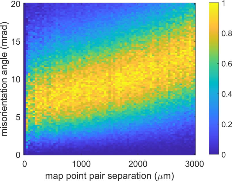
Materials 2020, 13, 2816 2 of 20
patterns, and thus has a direct influence on the precision of orientation data from the sample, the lattice
parameters, the sensitivity to pseudosymmetry issues, and the quality of phase discrimination,
among other issues [20,21,24–28]. In this way, the projection center is of key importance for the
principle of the EBSD method, but its quantitative influence on errors of the final EBSD orientation
data often is not completely transparent.
In the current paper, we describe the challenges for an accurate treatment of the projection
center, using the example case of low-magnification EBSD maps spanning areas of several square
millimetres on a silicon sample. In maps of these dimensions, the characteristic systematic changes of
the projection center within a map become particularly clear. Using measurements on single crystalline
silicon, we analyze the orientation consistency which can be achieved by the use of various models
for the position of projection center within the SEM scan. These results on relatively large scale maps
can be relevant, for example, to applications of silicon in microelectromechanical systems [29,30],
but also in general for materials with large grain sizes, as observed, e.g., in geological materials [31,32].
Because of the high perfection of single crystalline silicon, the magnitude of the inherent orientation
variations in the material can be neglected compared to the orientation variations which are caused
by the precision and accuracy of the EBSD pattern analysis itself. We assume that the Si material can
be described by a fixed, single true orientation, which is unknown, but which can be consistently
estimated from the EBSD orientation data. The observed, apparent, misorientations relative to this
fixed orientation are considered as an error signal. In order to quantify the precision of the EBSD
orientation determination in dependence on the projection center model, we adapt analytical tools
which have been developed for the description of small inter- and intragranular misorientations [33–35].
We quantify the precision of the EBSD orientation data by the resulting misorientations to the mean
orientation in a map, as well as the pairwise misorientation angles as a function of the map point pair
distance. These values will indicate how consistently the experimental projection center in different
parts of the map is approximated by the calibration models. Moreover, the statistical parameters which
we use for a description of the observed misorientation distributions can serve as figures of merit for
the precision of specific EBSD setups [36].
2. Experimental and Theoretical Details
2.1. Relationships between SEM Imaging Parameters and Projection Center
In order to motivate the specification of a mathematical model for the systematic change of the
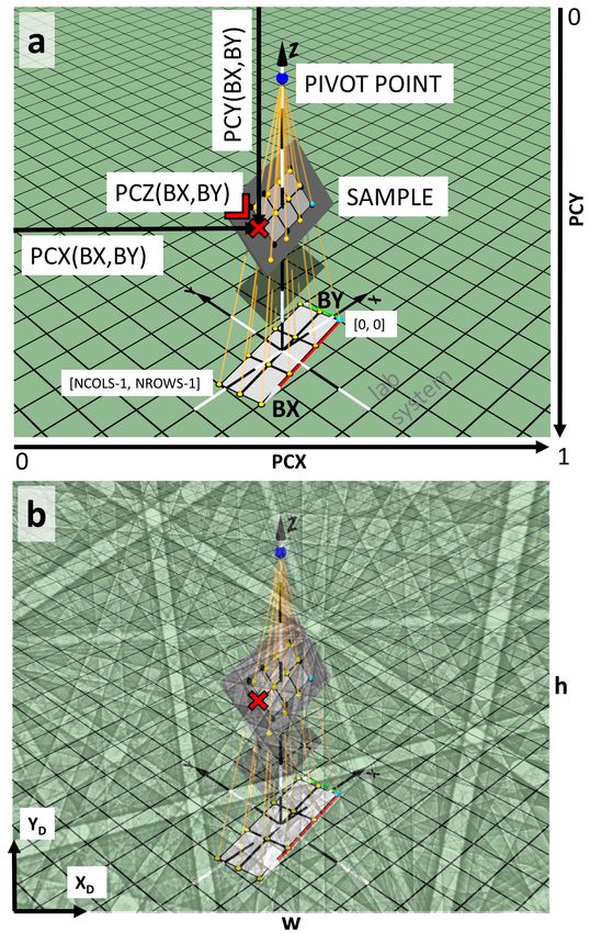
projection center on the sample, we recall the basic geometry of an EBSD experiment in Figure 1.
The task of the mathematical model will be to provide the 3D coordinates of the electron beam
positions on the sample relative to the detector screen, as a function of the current scan position within
the SEM scan (i.e., the column and row of a pixel in the resulting SEM image). In the following,
we will use the coordinate system conventions for EBSD as described in [4]. With respect to the
example Kikuchi diffraction pattern shown in Figure 1b with the relative projection center coordinates
of ( PCX, PCY, PCZ ) = (0.463, 0.516, 0.6), this convention means that the 3D geometric coordinates
relative to the lower left edge of the phosphor screen are XD = PCX · w, YD = (1 − PCY ) · h,
and ZD = − PCZ · h, with the physical screen dimensions of the detector as w = 31,600 µm and
h = 3w/4 for the full detector area (e− FlashHR , Bruker Nano GmbH, see also below). Thus, the electron
beam in Figure 1b is at XD = 14,630.8 µm to the right, YD = 16,305.6 µm up from the lower left corner
of the detection screen, and at ZD = −18,960.0 µm in front of the screen (i.e., below the drawing plane).
For the measurement in the SEM, we assume that, in order to scan a grid of image points on a
sample, the SEM scan generator deflects the beam from its neutral position into the direction to the
current map point, and that the bundle of the deflected beams can be assumed to originate from a
common virtual pivot point [37], see Figure 1a. Lower magnifications in the SEM correspond to larger
deflection angles of the incident electron beam. Due to the non-parallel directions of the incident beam
at different map positions, a regular grid of map points for a horizontal sample will be distorted if the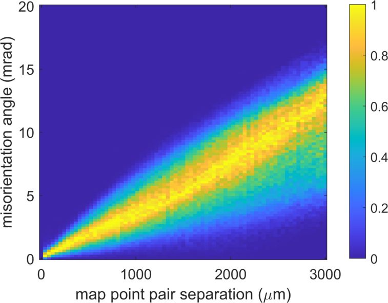
Materials 2020, 13, 2816                                                                               3 of 20

sample is tilted to a general position [12]. In this case, a square on the planar sample without tilt will
be transformed into a general quadrilateral on the tilted sample plane. The simplest distortion that can
be achieved by a systematic alignment procedure is a trapezoidal distortion, i.e., if the horizontal beam
scan is parallel to the tilt axis of the sample [12]. In the general situation, parallel lines of the scan on
the untilted sample will not stay parallel in the scan on the tilted sample; but straight lines between
scan points remain straight lines in the scan on the sample.
       The geometrical calibration of the EBSD measurement is given if we have determined all
parameters to specify the physical beam scan positions in relation to the EBSD screen as shown
in Figure 1b with a resulting Kikuchi pattern. As we tried to illustrate by this figure, the projection
center is not a “point in the Kikuchi pattern”, often called “pattern center”, but the projection center is
the location of the beam on the sample surface, measured relative to the detection screen, independent
of whether there is a Kikuchi diffraction pattern on the screen or not. This is why we prefer the term
“projection center” instead of “pattern center”. The projection center is essential to calibrate the correct
measurement of angular distances on the phosphor screen, and these angular measurements can also
be applied, for example, to a general electron scattering intensity distribution on the screen irrespective
of any diffraction effects [38]. As can be seen in Figure 1a, the treatment of the exact variation of the
projection center with the scan position in the map will become more and more relevant as the absolute
dimensions of the mapped area become a measurable part of the physical dimensions of the screen,
i.e., its physical width w and height h. Because the dimensions of the commercial EBSD system detector
screens are typically in the order of 30 mm, EBSD maps with dimensions of a few mm extension can
clearly be expected to show a strong influence, as the diffraction pattern will then move by visually
notable distances in the order of 10% of the detection screen. At the other extreme, for very small scan
dimensions, a sufficiently accurate projection center position is required for measurements of local
lattice parameters, including strain because the accuracy of these values is inherently limited by the
assumed projection geometry. For example, in [13], it has been estimated that an uncertainty of 0.005
in the projection center results in uncertainty of about 10−3 in the strain state, i.e., a variation of 0.1%
in lattice parameters.
       As a consequence of the influence of the scan size relative to the screen size, various levels
of approximations can be made in dependence on the necessary precision of the projection center
coordinates. The simplest assumption involves a constant effective projection center for the complete
map, which means that we would then neglect an actual variation in the order of ∆PC ≈ ∆x                   w ,
given by the EBSD map width ∆x relative to the EBSD screen width w. With physical screen sizes
w of the order of 30 mm, and allowing a maximal variation of the projection center in the order of
∆PC ≈ 0.001 to 0.005 in in the map, for example, we can estimate a maximum map dimension of
∆x = ∆PC · w ≈ (0.001 to 0.005) · 30 mm = 30 to 150 µm which would still meet the requirement of
the corresponding PC precision. A similar order of magnitude estimation results when we consider
that standard, low resolution EBSD patterns contain roughly 100 pixels on a 30 mm EBSD screen.
In this case, we obtain an effective pixel size of 300 µm, which is limiting the magnitude of shifts of
pattern features which can actually be detected. For example, if we optimistically postulate a sensitivity
to a 1/10th pixel shift in the projection center, this would correspond to a 30 µm shift of the beam.
These estimations show that, for high-magnification EBSD maps with dimensions of a few tens of
microns, the variation of the projection center in the map can be neglected in many applications. In the
limit of experiments aiming at absolute accuracy for local lattice parameters, however, the change
of projection center with map point position will always be relevant, independently of the spatial
map dimensions.

2.2. Projective Transformation Model
    The geometrical situation shown in Figure 1a can be described by projective geometry, where the
changes of the scan grid for different tilts of the sample can be treated by a projective transformation
using homogeneous coordinates [39]. A projective transformation allows for the fact that parallel lines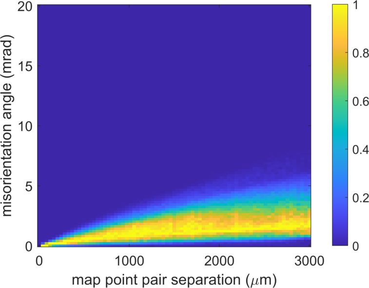
Materials 2020, 13, 2816 4 of 20
in the scan on the untilted sample will not stay parallel anymore on a tilted sample in the general
case. The special case of an affine transformation preserves the parallelism of lines, but still allows for
translations, scalings and shears, which can be a sufficient approximation in many cases.
Figure 1. Illustration of the 3D geometry relevant to the EBSD projection center. (a) projection geometry
of the SEM beam scanning the sample as seen from an EBSD detector screen plane in a general
position. The scan pattern shows the combined effects of scan rotation and the sample tilt;
(b) correspondingly simulated Kikuchi pattern with ( PCX, PCY, PCZ ) = (0.463, 0.516, 0.6) as a
semi-transparent overlay on the screen plane. The projection center is at the position of the electron
beam on the sample, PCZ units of the screen height behind the pattern, measured normal to the screen
plane. The decreased visibility of the scan geometry in (b) is intended to remind the reader that the
scan geometry is usually hidden by the detection screen with the Kikuchi diffraction pattern.
Under these conditions, the relationship between the 2D beam scan indices [ BX, BY ] and the 3D
projection center values [ PCX, PCY, PCZ ] can be described by a projective transformation P
P11 P12 P13
P P22 P23
P = 21 (1)
P31 P32 P33
P41 P42 1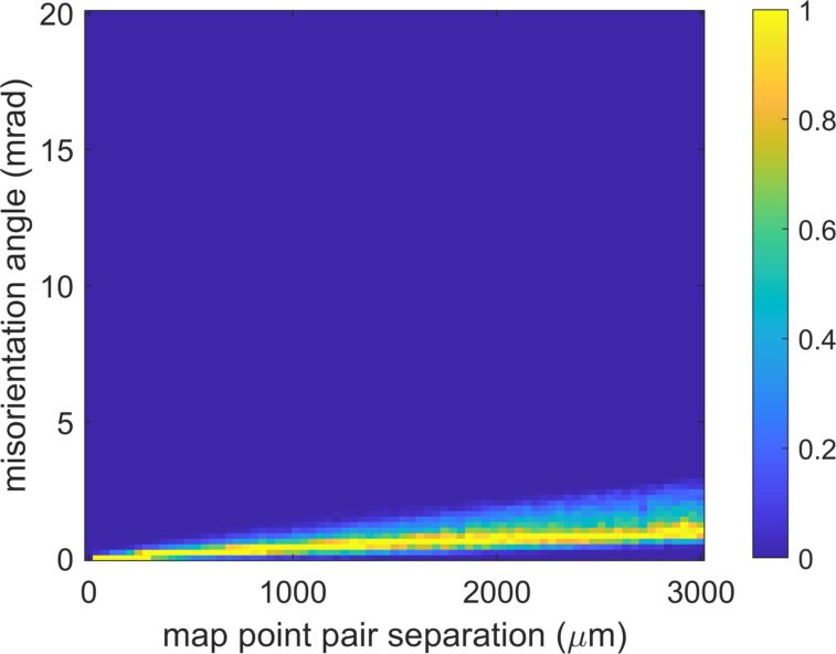
Materials 2020, 13, 2816 5 of 20
where the matrix P takes the homogeneous column vectors b = ( BX, BY, 1) T to the homogeneous
vectors c( BX, BY ) = ( PCX, PCY, PCZ, 1) T via:
P · b = w = w · c = w · ( PCX, PCY, PCZ, 1) T = (w1 , w2 , w3 , w4 ) T (2)
As can be seen in Equation (2), the result w of the projective transformation P is not c directly,
but c scaled by a real factor w which depends on b. The final projection center values can be obtained
from w by dehomogenization, i.e., by dividing by the fourth component of w (for w4 6= 0):
PCX = w1 /w4 PCY = w2 /w4 PCZ = w3 /w4 (3)
A special case results when setting P41 = P42 = 0, leading to an affine transformation A
A11 A12 A13
A A22 A23
A = 21 (4)
A31 A32 A33
0 0 1
which leaves the 4th component of the homogeneous projection center vector at w = 1:
A·b = c (5)
From observed pairs of beam scan grid indices and projection center vectors, a best-fit affine
transformation matrix A can be found by least-squares solution to a linear matrix equation:
BE AT = CE (6)
where B E and C E are n × 3 (n ≥ 3) matrices with rows i = 1, . . . , n of the experimental data points
(i ) (i )
b E = ( BXi , BYi , 1) and c E = ( PCXi , PCYi , PCZi , 1), which are the beam scan grid indices and
observed projection center values, respectively. To solve the overdetermined matrix Equation (6) for
A T , we have used the leastsqr outine available in the numpy.linalg Python package [40].
The affine projection center fit has also been used in [20] using a similar pattern matching
approach as described here. For the more general projective transformation P, the determination
of the transformation matrix from to observed points is a well known problem in computer
vision [39]. Various methods for finding the best-fit projective transformation for point sets in
3D (i.e., 4D homogeneous coordinates) are discussed in [41]. For the current application, we have
implemented an iterative optimization routine to find a projective matrix P by starting from an affine
transformation and minimizing the root mean square deviation to the experimental projection center
vector components. We have found this approach to work well when P41 and P42 are very small
compared to all other elements and the effect of P remains close to an affine transformation.
2.3. Kikuchi Pattern Matching for Projection Center Calibration
(i )
In order to obtain the experimental estimations c E = ( PCXi , PCYi , PCZi , 1) of the PC coordinates
from the experimental Kikuchi patterns, individual values for the orientation and the projection
(i )
center c E of a map point i where determined by a best-fit pattern matching approach as described
in [28,42]. The best fit parameters were determined at the maximum of the normalized cross correlation
coefficient (NCC) between the simulated pattern and the experimental pattern. In comparison to
other available measures used for Kikuchi pattern matching, the NCC is very robust to changes
in brightness and contrast in the analyzed Kikuchi patterns, among other useful properties of the
NCC [43–46]. The pattern matching procedure compares background-corrected Kikuchi patterns
which have been normalized to a mean of zero and unit standard deviation [47]. As starting valuesMaterials 2020, 13, 2816 6 of 20
for the optimization procedure, we used the values of the local orientation and PC as given by the
EBSD system software (Bruker Esprit 1.94, Bruker Nano GmbH, Berlin, Germany). The starting
values which were optimized using the Nelder-Mead (NM) algorithm as implemented in the NLOPT
nonlinear optimization package [48]. In order to test the convergence, the NM optimization for each
map point was restarted several times with different initial values changed by random deviations,
i.e., orientations within one degree misorientation angle, and the PC values changed in a range of
±0.02. We found that a number of five restarts were sufficient in most cases. In the present study,
we used experimental Kikuchi patterns with a resolution of 400 × 300 pixels, which were resampled
to a resolution of 800 × 600 pixels to reduce possible discretization effects in the projection center
optimization process.
In a first step, the optimization procedure varied the orientation parameters and the projection
center coordinates on a 7 × 7 subset of points covering the complete map. Taking the NCC as a quality
measure, outliers to be discarded can be defined as data points with a NCC below a certain threshold.
The resulting values for the projection coordinates where then fitted to an affine and a projective
transformation as discussed above. A consistent calibration of the projection center for all points in the
map is finally given by the nine parameters of the affine projection matrix A of Equation (4) and the 11
parameters of the projective projection matrix P of Equation (1), respectively.
After the projection center calibration matrices A and P have been determined in the first step,
we subsequently optimized the orientation values for all points in the map, fixing the local projection
center coordinates at the scan points [ BX, BY ] as given by the calibration matrices. Only the orientation
parameters (Euler angles) were varied in this final optimization step. On a single-crystalline sample
without any internal orientation changes in the material, an idealized analysis should result in the
actual orientation of the material, which would be identical for all data points in the map of the
single crystal. The limited precision and accuracy of the complete EBSD data analysis pipeline,
however, will result in systematic and random errors of the actual experimental orientation data,
even from a nearly perfect material. If we can expect that the orientations vary randomly around a
mean orientation, we can take this mean orientation as the reference orientation. While we cannot
conclude on a possible systematic deviation of this mean orientation data from the true orientation
of the material, we can analyze the precision of the projection center calibration by the spread in
the final, optimized orientations relative to the mean orientation. We can expect that an improved
precision of the projection geometry should lead to less spread of the orientation data around the
average orientation in the EBSD map of a single-crystalline material.
2.4. EBSD Measurements
The EBSD measurements have been performed using a field-emission gun scanning electron
microscope (FEG-SEM) LEO 1530VP (Zeiss, Oberkochen, Germany). Using the high-current mode and
a 120 µm aperture, the Shottky field emitter delivered a probe current of about 10, . . . , 12 nA in high
vacuum mode.
For the EBSD-pattern acquisition an e− FlashHR (Bruker Nano GmbH, Berlin, Germany, nominal
CCD-chip resolution: 1600 × 1200 pixels) was used. The analyzed and stored raw patterns were 8-bit
gray-scale images with a size of 400×300 pixels. The dwell times per pattern were 15 ms. We did not
apply any frame averaging. For the EBSD orientation data analysis, we applied the internal EBSD
system software (Esprit 1.94), as well as the MTEX toolbox [49].
The sample used in this study was obtained from a commercial Si(001) wafer as delivered,
without any further sample preparation. The sample was deliberately mounted in a slightly tilted
position relative to the surface of the sample holder, in order to include the effect of a general tilt
in the projection center calibration. The Si sample was imaged at low magnification (nominally
85×) with 100 × 75 map points at a nominal 40 µm step size, leading to a total mapped area of
4 mm × 3 mm extension.Materials 2020, 13, 2816 7 of 20
3. Results
3.1. Projection Center Calibration
For the calibration of the projection center in the map, we carried out the pattern matching
procedure as described above for a subset of 7 × 7 grid points across the map. In Figure 2, we show the
results for the four corner points of the scan having a total of 100 columns and 75 rows. The beam scan
indices [ BX, BY ] correspond to the column BX and row BY in the scan. The overall level of agreement
between simulations and experiment can be seen by the Kikuchi patterns, marked “S” (simulation) and
“E” (experiment), respectively. The pattern similarity is quantified by the normalized cross correlation
coefficient r, which is mainly in the range 0.6 < r < 0.7 for the current sample. In the center of
Figure 2, we show the full r-map which resulted after the orientation refinement as will be discussed
below. Dark spots indicate positions of lower quality Kikuchi patterns due to contamination on the
sample surface. The best-fit projection center coordinates PCX, PZY, PCZ at the example points are
shown in color in Figure 2. In agreement with the geometry of the scan relative to the EBSD screen [4],
the Kikuchi patterns can be seen to move to the left with increasing BX, and upwards with increasing
BY. Because the vertical movement with increasing BY also moves the beam away from the screen on
the tilted sample, this also leads to an increasing PCZ, and the patterns in the lower row also appear
zoomed-in, as is visible by the slightly broader Kikuchi bands. The key topic of the present paper
is to quantify the existing effect of this observed movement of the Kikuchi patterns on the resulting
orientation data. While the imaged Kikuchi patterns change due to the movement of the electron
emission spot relative to the screen, the orientations at these positions on the silicon sample remain
essentially constant. The consistency of the resulting EBSD orientation data can be judged by how well
the constraint of an identical orientation is fulfilled on the mapped positions. Based on Figure 2, it can
be supposed that the measurable variations would be largest if the resulting orientations from the
corner regions of the map are compared relative to each other because then also the relative changes in
the Kikuchi patterns are largest.
The set of 7 × 7 calibration points resulted in pairs of the experimental data points
(i ) (i )
b E = ( BXi , BYi , 1) and c E = ( PCXi , PCYi , PCZi , 1) with i = 1, . . . , 49. Using a threshold value
of rmin = 0.65, the experimental data points were fitted to the affine and projective transformations as
described above. The results are shown in Figure 3. In the lower right panels of (a) and (b), we show
the histograms of the absolute difference between the experimental and the fitted projection center
vectors, and the respective transformation matrices. For calculation of the error values shown in the
histograms in Figure 3, we scaled PCX to also correspond to the image height, in order to measure
all values relative to the same reference length. The resulting root mean square deviation (RMSD)
between experiment and simulation is 0.00120 for the fit of an affine transformation, and 0.00028 for
the fit to the projective transformation model, indicating an increase of the error by a factor larger than
4 for the affine model. Taking the absolute height of the EBSD detector area for the image as 23.7 mm,
the RMSD values would correspond to 28.4 µm for the affine model and 6.6 µm for the projective model,
which illustrates the size of the systematic error introduced by a limitation to an affine transformation.
The consistently better fit of the projective model can also be noticed in the panels which show 2D maps
of pairs of the three projection center coordinates. The missing nine grid points are ouliers as defined
as having an NCC less than the minimum value rmin = 0.65. The projective transformation takes into
account that the scan grid lines on a tilted sample are not parallel anymore. In contrast, the affine
transformation model conserves parallelism and can only treat scalings and shears. The map of PCY
vs. PCZ should be a straight line if the sample would have rotated only around the x-axis, and from
the slope of the we can estimate the corresponding sample tilt relative to the detector. The estimation
using linear regression leads to a tilt angle of ϑxLR = 23.12° of the sample plane normal in the detector
(y, z)-plane. Taking into account a possible small tilt of the EBSD detector, as well as of the sample
mount, the value of ϑxLR is compatible with the nominal 70° sample tilt, which is measured relative to
the microscope z-axis. In Figure 3, we see a very systematic deviation of the experimental data fromMaterials 2020, 13, 2816 8 of 20
the line in the relationship between PCY and PCZ. This is due to an additional small tilt of the sample
plane, which makes the sample plane normal to point slightly away from the (y, z)-plane, i.e., the
sample plane normal is not at a right angle relative to the x-axis of the detection screen.
E
S
[0, 0] [99, 0]
r=0.691 r=0.687
0.57252 0.43125
0.21835 0.22852
0.77492 0.77720
PCX
BY PCY
PCZ
0.56577 0.43561
0.08933 0.10001
0.83027 0.83302
[0,74] BX [BX,BY]=[99,74]
r=0.667 r=0.683
E
S
Figure 2. Projection center (PC) pattern matching results for the corner points of the map.
The experimental patterns are marked by “E” and the corresponding best-fit simulations are shown by
“S”. The best-fit PC values PCX, PZY, PCZ are shown in color, below the beam scan indices [ BX, BY ]
and the value of the normalized cross-correlation coefficient r. In agreement with the geometry of the
scan relative to the EBSD screen [4], the Kikuchi patterns can be seen to move to the left with increasing
BX, and upwards with increasing BY. Because the vertical movement with increasing BY also moves
the beam away from the screen on the tilted sample, increasing PCZ, the patterns in the lower row
also appear magnified, as can be seen by the slightly broader Kikuchi bands. The full map of r-values
resulting during the final orientation refinement shown in the center.Materials 2020, 13, 2816 9 of 20
(a) fit of PC to an affine transformation Af it
(b) fit of PC to a projective transformation Pf it
Figure 3. Fit of transformation matrices to the individual experimental projection center (PC)
coordinates. The small black points are the experimental data points, and the larger gray filled
circles are the respective fit results according to (a) the affine transformation matrix A f it and (b) the
projective transformation matrix P f it shown in the lower right panels. Experimental data points were
measured on a 7 × 7 subgrid and selected according to a minimum allowed cross-correlation coefficient
rmin = 0.65. This resulted in the 41 calibration points as shown in the figure.Materials 2020, 13, 2816 10 of 20
The resulting transformation matrices allow for describing the general orientation of the sample
plane relative to detector. This can be achieved by calculating the images of the points [0, 0, 1], [1, 0, 1],
and [0, 1, 1], which span the resulting scanning plane. We measure the orientation of the scanning
plane in the detector system [4], for a sample normal reference direction along the positive z-axis
(i.e., the detector screen normal pointing away from the sample). For the experimental data above, we
find that the normal vector of the scanning plane is rotated by ϑx = 23.24° from the (z, x )-plane (towards
positive y) and by an angle τy = −2.16° relative to the (y, z)-plane (towards negative x). Both the affine
and the projective transformation model give the same sample plane normal direction within the
precision stated above. This observation is consistent with the fact that both types of transformations
conserve the co-planarity of the scan points. The difference of the two transformation models is mainly
on the position of the map points within the sample plane, i.e., the projective transformation allows
parallel lines in the beam scan grid to become non-parallel within the sample plane.
3.2. Orientation Analysis
The effect of the different calibrations of the projection center in the map can be seen by an analysis
of the resulting orientation data. This allows us to quantify the influence of the observed movement of
the Kikuchi patterns on the orientation data from nearby map points (the local orientation precision),
as well as on the changes of orientations of map points as a function of their mutual separation (global
orientation precision).
3.2.1. Local Orientation Precision
The local variation in the orientation data can be quantified by misorientation values in the
neighborhood of each map point [50]. In Figure 4, we show the histograms of the Kernel Average
Misorientation angle (KAM) to the nearest neighbor in the orientation maps (calculated using the first
order KAM angles as implemented in MTEX 5.2.8 [51]). The initial values which were obtained using
the orientation from the EBSD system software are shown in Figure 4a, compared to the KAM values
obtained from the refined orientation map using the affine transformation model in Figure 4b and
the projective transformation model in Figure 4c. Qualitatively, we can see that the pattern matching
based values in (b) and (c) are almost two orders of magnitude lower than the result in (a), noting that
the angular scale goes up to 2 degrees in (a) compared to the maximum range of 0.02 in (b) and
(c). The distribution of the KAM angles in the histograms are summarized by the median and 95th
percentile values given in Table 1. While the projective transformation model results in marginally
lower KAM values than the affine transformation model, the most significant difference is seen
relative to the raw orientation data that was provided by of the EBSD system software. Comparable
improvements of the KAM values have been shown previously for measurements on Si samples and
map areas of about 1 mm2 in [20]. We note that different types of EBSD systems using various data
analysis approaches can be expected to provide the raw orientation data with their different typical
precision [52–55].
Because the variation of the projection center position is small from one map point to its neighbor,
the local KAM values do not show a strong dependence of the spatial position in the map. The error of
the local projection center position will be approximately constant for neighboring data points and
thus the resulting orientations and the corresponding local KAM do not change very much locally.
We have observed that the only systematic features are at the contamination spots, and this is why the
KAM maps are not shown explicitly. The KAM histograms in Figure 4 convey the key information.Materials 2020, 13, 2816 11 of 20
(a) raw data from EBSD system software
(b) affine PC model
(c) projective PC model
Figure 4. Histograms of the Kernel Average Misorientation angle for the orientation maps resulting
from different analysis approaches. (a) raw data from EBSD system, (b) refined orientations using
affine PC calibration, (c) refined orientations using projective PC calibration. Note that the x-axis limit
in the top panel ( (a) is larger by a factor of 100 compared to the other two panels.Materials 2020, 13, 2816 12 of 20
Table 1. Characteristic values of the histograms ot the Kernel Average Misorientation Angle shown in
Figure 4.
Orientation Data KAM Median KAM 95th Percentile
Esprit 1.94 0.4100° 0.690°
Affine PC 0.0074° 0.011°
Projective PC 0.0058° 0.010°
3.2.2. Global Orientation Precision
The EBSD orientation data in the present study can effectively be considered to originate
from a single large grain of nearly perfect Si. This makes it possible to apply some well-known
characterization concepts for intragranular orientation variations in materials to describe the apparent,
spatially dependent orientation variations which are induced purely by an inaccurate assumption for
the projection center in the EBSD data analysis.
A useful measure to illustrate the variation of orientations in the map is the misorientation angle
relative to the mean orientation [34,35,49,56,57]. In Figure 5, we show the maps of the misorientation
angle relative to the mean orientation, which result from using the different calibration approaches for
the projection center. As we can see by a comparison of the angular scale in Figure 5a to the scales in (b)
and (c), the pattern matching orientation refinement in (b,c) reduces the overall, apparent, orientation
variation in the map by about an order of magnitude. The comparison of the affine model applied in (b)
to the results from the projective model in (c) shows that the projective model leads to a significantly
reduced spatial orientation deviation, with the largest difference remaining in the upper left corner
of the map. This improvement shows the signifance of the projective calibration in terms of the total
orientation consistency in the map. In comparison, the local KAM values are not influenced as critically
by the choice of an affine or projective model, as we have seen in Figure 4.
The maps in Figure 5 can be quantitatively described by an analysis of the components of the
rotation vector relative to the mean orientation. The corresponding rotation vectors ~Θ are defined
to point into the direction of the rotation axis and have a length corresponding to the rotation angle
(see e.g., Equation (2.51) and Chapter 3 in [58]). The advantage of the rotation vector is that it linearizes
the space of rotations for small rotations, using the components Θ x , Θy , Θz as coordinates, i.e., see the
discussion of the Lie group SO(3) in [58]. This makes it possible, for example, to analyze small random
rotations in terms of Gaussian distributions for Θ x , Θy , Θz (note that this is not valid for a rotation
description by Euler angles). In the context of EBSD, the rotation vector and closely related quantities
have been used before to analyze plastic deformations relative to the mean orientation in individual
grains [34,56,59,60].
For the measurement of the Si sample, the histograms of the rotation vector components Θ x , Θy , Θz
and of the resulting absolute value of the misorientation angle ω = (Θ2x + Θ2y + Θ2z )1/2 are shown in
Figure 6. On the left side, in panels (a,c,e), we show the histograms resulting for the orientations from
the EBSD system software. It can be seen that the histograms of the rotation vector components for
the raw data are very well described by Gaussian distributions with a mean of zero and a standard
deviation σraw ≈ 5 mrad, which are shown as black lines. On the right side, in panels (b,d,f), the rotation
vector components are shown which result from orientation refinement using full pattern matching
with the projective calibration. These distributions have a spread which is about an order of magnitude
smaller than the raw EBSD data, as can be seen by the standard deviations near σ proj ≈ 0.4 mrad
around a mean value near zero. The shape of the refined distributions deviates from a Gaussian shape
more than the EBSD raw data, and the spread is slightly different for the Θ x , Θy , Θz components.
We assign the detailed shape of these distributions to a remaining influence of discretization effects
on the pattern fit, which depend on the specific orientation of the Si sample, the resolution of the
measured patterns and the solid angle of the captured diffraction patterns [61], in addition to the limits
of the theoretical approach itself which neglects or approximates a range of experimentally observableMaterials 2020, 13, 2816 13 of 20
pattern details. These details include the excess-deficiency effects [62] and higher-order Laue zone
rings [63], which require numerically more expensive simulations [64].
(a) raw data from EBSD system software
(b) affine PC model
(c) projective PC model
Figure 5. Maps of the misorientation angle to the mean orientation. (a) raw data from EBSD system, (b)
refined orientations using affine PC calibration, (c) refined orientations using projective PC calibration.
Scale in degrees, note that the scale for the raw data in (a) is increased by a factor of 10.Materials 2020, 13, 2816 14 of 20
(a) orientation data from EBSD system software (b) projective PC model
(c) (d)
(e) (f)
(g) fit to Maxwell-Boltzmann distribution (h) fit to Maxwell-Boltzmann distribution
Figure 6. (a–f) Histograms of the rotation vector components of the misorientation relative to
the mean orientation, (a,b) Θ x , (c,d) Θy , (e,f) Θz ; and (g,h) the histograms of the misorientation
angles ω. The black solid lines correspond to fits of Gaussian distributions (top three rows) and
Maxwell–Boltzmann distributions (lower row) with the standard deviations shown on top of each plot.
The left column shows the data for the raw EBSD maps, the right column shows the results from the
orientation data which was refined by the projective model. Note that the angular scale for the left
column is ten times larger than for the right column.Materials 2020, 13, 2816 15 of 20
In the bottom row of Figure 6, we show that the histograms of the misorientation angle ω can
be fitted by a Maxwell-Boltzmann distribution, which is the theoretical distribution of the square
root of a sum of three random variables which are independently distributed according to Gaussian
distributions with mean value zero and the same standard deviation σM :
r !
2 ω2 ω2
p(ω ) = 3
exp − 2 (7)
π σM 2σM
The Maxwell-Boltzmann distribution is also useful as the limiting case of a general class of distributions
used for the statistical description of rotations [65]. If the rotation vector components cannot be
assumed to be normally distributed with approximately the same standard deviation and mean zero,
other distributions for the misorientation angle ω = (Θ2x + Θ2y + Θ2z )1/2 will result. For example, if the
misorientations are effectively two-dimensional, a Rayleigh distribution [34] is obtained.
Applying a least square fit to the Maxwell-Boltzmann distribution in Equation (7), we find
raw = 5.1 mrad for the raw EBSD system orientation data, while the refined orientation data shows a
σM
proj
value of σM = 0.40 mrad. With respect to the differences which are seen between the orientation maps
af f
of the affine model and the projective model in Figure 5, we find an increased value of σM = 0.69 mrad
for the affine model using the same analysis. This corresponds to an increase in the spread of
orientations σM by a factor of 1.7 between the projective and the affine calibration, and an increase of a
factor of 12.7 for the raw EBSD system data.
As can be seen in Equation (7), the Maxwell–Boltzmann distribution depends only on one
parameter, namely σM , which, in our application, can be seen to approximately describe an effective
standard deviation of the components of the misorientation vectors relative to a true mean orientation.
Because of this straightforward statististical meaning, the value of σM could be used as a key parameter
to describe the orientation precision of a specific EBSD setups. We can expect that σM will depend
on the specific combination of SEM, the EBSD system hardware, and the data analysis software,
when carried out on easily available Si samples measured in given reference orientations [36].
In general, the spread of orientations described by σM will also depend on the spatial distance
of the map points which have been used to calculate the distribution of the misorientation angles
ω. It can be speculated that pairs of map points which are separated by large distances will also
tend to show larger misorientations. We have quantified this expectation by calculating the pairwise
misorientation angles for a given number of randomly selected pairs from the map, and counting the
number of pairs within specific intervals of distances and misorientation angles as two-dimensional
histograms. The resulting two-dimensional histograms for 106 pairs from the Si map are shown in
Figure 7. In these figures, the distributions of the misorientation angle in each given bin of map point
pair separation are normalized to the maximum of the counts for all angles in that bin. In this way,
the distance-dependend shift of the maximum and the changes in the width of the distribution is
emphasized. The spatial step size in the histogram is 40 µm. For the raw EBSD data, it can be seen
that the dominating misorientation values are between 5 and 10 mrad for map point separations in
the order of 100 µm, and this interval rises towards values between 10 and 15 mrad for a separation
near 3 mm. As can be seen in panel (b), the orientation precision of nearby points can be improved
by pattern matching using an unrefined projection center as given by the EBSD system software,
but the misorientation at a large distance still tends to similar values as in the raw data. For the
affine PC model shown in (c), the misorientation angles stay below 5 mrad, and in (d) we can see
that the projective model has a still sharper distribution with angles predominantly below 1 mrad
deviation. Thus, the projective model for the projection center also leads to the least increase in relative
misorientation between spatially separated data points which nominally have the same orientation.
We note that this type of information about the spatially changing, systematic orientation errors is
usually not accessible in measurements from polycrystalline maps because the separated points thenMaterials 2020, 13, 2816 16 of 20
are very likely to be in different grains. In that situation, the locally changing systematic orientation
error is masked by the locally changing grain orientations.
(a) orientations from EBSD system software (b) PC from EBSD system software
(c) affine PC fit (d) projective PC fit
Figure 7. Distributions of the relative misorientation angle between pairs of map points, as a function
of the map point pair separation for different projection center models. (a) raw orientations as given by
the EBSD system software, (b) refined orientations by pattern matching using the PC calibration of the
EBSD system software, (c) refined orientations using the affine PC calibration, (d) refined orientations
using the projective PC calibration. The distributions are normalized to the maximum value of the
misorientation angle distribution at each distance (bin width 40 µm).
4. Conclusions
We have demonstrated the use of a projective transformation model for the calibration of the
projection center in EBSD maps of large spatial dimensions, involving low magnifaction modes in the
scanning electron microscope.
Using measurements on single-crystalline Si samples, we have shown that, compared to an affine
transformation, the projective transformation model leads to a decreased spread of misorientation
angles relative to the mean orientation when the orientations are refined using a full pattern
matching approach.
For the combination of EBSD system and SEM which was used in the present study, this approach
leads to an improvement of the local orientation precision by of about two orders of magnitude (as seen
by the KAM maps), and to an improvement in global orientation precision by one order of magnitude
(as seen by the misorientation angles relative to the mean orientation).
Ultimately, the approach of fitting the projection center to simulated Kikuchi patterns is limited
by the ability of the simulation to take into account all relevant experimental effects. For example,
the excess-deficiency effects have not been included in the current simulation model [62]. As has beenMaterials 2020, 13, 2816 17 of 20
discussed above, the projection center is essentially related to the purely geometrical relationships
in the measurement setup. In order to analyze the absolute precision of the projection center,
alternative determinations of the projection geometry could use methods which are independent
of the observation of any Kikuchi patterns from the sample, such as shadow casting methods [6,15] or
single-crystalline detectors like those discussed in [19].
The problem of the dependence of the projection center on the position within the beam scan is
closely related to the observed spatial distortions of EBSD maps when mapping large sample areas
by assembling a number of smaller sub-maps into a larger mosaic. As we have shown, the projective
transformation model can provide an improved description of the scan geometry in larger EBSD maps,
which could help to reduce the number of maps which would need to be stitched together for a given
sample area. The projective transformation model is also relevant to SEM in-situ testing setups for
mechanical properties of materials, where deformations are measured on large sample areas [66,67].
A precise correction of the spatial distortions will also require the treatment of the electron lens
distortions which lead to a deviation from the purely projective distortion model. Methods to correct
for these additional influences are well known for optical systems in computer vision [39], and could
be implemented by transforming the initial scan incides [ BX, BY ] according to the radial and tangential
disortions caused by the electron optics [68]. The investigation of such additional corrections in the
future is also expected to further improve the orientation consistency in EBSD maps.
Author Contributions: Conceptualization, A.W.; methodology, A.W. and G.N.; software, A.W.; validation,
G.C. and T.T.; formal analysis, A.W.; investigation, G.N. and G.C.; resources, G.N. and P.B.; data curation,
A.W.; writing—original draft preparation, A.W.; writing—review and editing, A.W., G.N., G.C., T.T., and P.B.;
visualization, A.W.; supervision, P.B.; project administration, G.C., T.T., and P.B.; funding acquisition, G.C. and
A.W. All authors have read and agreed to the published version of the manuscript.
Funding: This research was funded by Polish National Agency for Academic Exchange (NAWA) Grant No.
PPI/APM/2018/1/00049/U/001 and PPN/ULM/2019/1/00068/U/00001.
Acknowledgments: We thank Michaela Buchheim and Romeo Saliwan Neumann (BAM) for valuable
technical support.
Conflicts of Interest: The authors declare no conflict of interest. The funders had no role in the design of the
study; in the collection, analyses, or interpretation of data; in the writing of the manuscript, or in the decision to
publish the results.
References
1. Schwartz, A.J.; Kumar, M.; Adams, B.L. (Eds.) Electron Backscatter Diffraction in Materials Science;
Kluwer Academic/Plenum Publications: New York, NY, USA, 2000.
2. Engler, O.; Randle, V. Introduction to Texture Analysis: Macrotexture, Microtexture, and Orientation Mapping,
2nd ed.; CRC Press: Boston, MA, USA, 2009.
3. Palache, C. The Gnomonic Projection. Am. Mineral. 1920, 5, 67–80.
4. Britton, T.; Jiang, J.; Guo, Y.; Vilalta-Clemente, A.; Wallis, D.; Hansen, L.; Winkelmann, A.; Wilkinson, A.
Tutorial: Crystal orientations and EBSD—Or which way is up? Mater. Charact. 2016, 117, 113–126,
doi:10.1016/j.matchar.2016.04.008.
5. Venables, J.A.; Bin-Jaya, R. Accurate microcrystallography using electron back-scattering patterns.
Philos. Mag. 1977, 35, 1317–1332, doi:10.1080/14786437708232955.
6. Biggin, S.; Dingley, D.J. A general method for locating the X-ray source point in Kossel diffraction. J. Appl.
Crystallogr. 1977, 10, 376–385, doi:10.1107/s0021889877013806.
7. Dingley, D.J.; Longden, M.; Weinbren, J.; Alderman, J. Online Analysis of Electron Back Scatter Diffraction
Patterns. 1. Texture Analysis of Zone Refined Polysilicon. Scanning Microsc. 1987, 1, 451–456.
8. Baba-Kishi, K.Z. Measurement of crystal parameters on backscatter Kikuchi diffraction patterns. Scanning
1998, 20, 117–127, doi:10.1002/sca.1998.4950200210.
9. Krieger Lassen, N.C.; Bilde-Sørensen, J.B. Calibration of an electron back-scattering pattern set-up. J. Microsc.
1993, 170, 125–129, doi:10.1111/j.1365-2818.1993.tb03331.x.
10. Krieger Lassen, N.C. Source point calibration from an arbitrary electron backscattering pattern. J. Microsc.
1999, 195, 204–211, doi:10.1046/j.1365-2818.1999.00581.x.Materials 2020, 13, 2816 18 of 20
11. Carpenter, D.A.; Pugh, J.L.; Richardson, G.D.; Mooney, L.R. Determination of pattern centre in EBSD using
the moving-screen technique. J. Microsc. 2007, 227, 246–247, doi:10.1111/j.1365-2818.2007.01807.x.
12. Nolze, G. Image distortions in SEM and their influences on EBSD measurements. Ultramicroscopy 2007,
107, 172–183, doi:10.1016/j.ultramic.2006.07.003.
13. Britton, T.B.; Maurice, C.; Fortunier, R.; Driver, J.H.; Day, A.P.; Meaden, G.; Dingley, D.J.; Mingard, K.;
Wilkinson, A.J. Factors affecting the accuracy of high resolution electron backscatter diffraction when using
simulated patterns. Ultramicroscopy 2010, 110, 1443–1453, doi:10.1016/j.ultramic.2010.08.001.
14. Maurice, C.; Dzieciol, K.; Fortunier, R. A method for accurate localisation of EBSD pattern centres.
Ultramicroscopy 2011, 111, 140–148, doi:10.1016/j.ultramic.2010.10.007.
15. Mingard, K.; Day, A.; Maurice, C.; Quested, P. Towards high accuracy calibration of electron backscatter
diffraction systems. Ultramicroscopy 2011, 111, 320–329, doi:10.1016/j.ultramic.2011.01.012.
16. Basinger, J.; Fullwood, D.; Kacher, J.; Adams, B. Pattern center determination in electron backscatter
diffraction microscopy. Microsc. Microanal. 2011, 17, 330–340, doi:10.1017/S1431927611000389.
17. Alkorta, J. Limits of simulation based high resolution EBSD. Ultramicroscopy 2013, 131, 33–38,
doi:10.1016/j.ultramic.2013.03.020.
18. Ram, F.; Zaefferer, S.; Raabe, D. Kikuchi bandlet method for the accurate deconvolution and
localization of Kikuchi bands in Kikuchi diffraction patterns. J. Appl. Cryst. 2014, 47, 264–275,
doi:10.1107/s1600576713030446.
19. Vespucci, S.; Naresh-Kumar, G.; Trager-Cowan, C.; Mingard, K.P.; Maneuski, D.; O'Shea, V.; Winkelmann, A.
Diffractive triangulation of radiative point sources. Appl. Phys. Lett. 2017, 110, 124103, doi:10.1063/1.4978858.
20. Friedrich, T.; Bochmann, A.; Dinger, J.; Teichert, S. Application of the pattern matching approach for EBSD
calibration and orientation mapping, utilising dynamical EBSP simulations. Ultramicroscopy 2018, 184, 44–51,
doi:10.1016/j.ultramic.2017.10.006.
21. Pang, E.L.; Larsen, P.M.; Schuh, C.A. Global optimization for accurate determination of EBSD pattern centers.
Ultramicroscopy 2020, 209, 112876, doi:10.1016/j.ultramic.2019.112876.
22. Lafond, C.; Douillard, T.; Cazottes, S.; Steyer, P.; Langlois, C. Electron CHanneling ORientation Determination
(eCHORD): An original approach to crystalline orientation mapping. Ultramicroscopy 2018, 186, 146–149,
doi:10.1016/j.ultramic.2017.12.019.
23. Lafond, C.; Douillard, T.; Cazottes, S.; Graef, M.D.; Steyer, P.; Langlois, C. Towards large scale orientation
mapping using the eCHORD method. Ultramicroscopy 2020, 208, 112854, doi:10.1016/j.ultramic.2019.112854.
24. Nolze, G.; Winkelmann, A. Exploring structural similarities between crystal phases using EBSD pattern
comparison. Cryst. Res. Technol. 2014, 49, 490–501, doi:10.1002/crat.201400091.
25. Winkelmann, A.; Nolze, G. Point-group sensitive orientation mapping of non-centrosymmetric crystals.
Appl. Phys. Lett. 2015, 106, 072101, doi:10.1063/1.4907938.
26. Chen, Y.H.; Park, S.U.; Wei, D.; Newstadt, G.; Jackson, M.A.; Simmons, J.P.; De Graef, M.; Hero, A.O. A
Dictionary Approach to Electron Backscatter Diffraction Indexing. Microsc. Microanal. 2015, 21, 739–752,
doi:10.1017/s1431927615000756.
27. Hielscher, R.; Bartel, F.; Britton, T.B. Gazing at crystal balls: Electron backscatter diffraction pattern analysis
and cross correlation on the sphere. Ultramicroscopy 2019, 207, 112836, doi:10.1016/j.ultramic.2019.112836.
28. Winkelmann, A.; Jablon, B.M.; Tong, V.S.; Trager-Cowan, C.; Mingard, K.P. Improving EBSD precision by
orientation refinement with full pattern matching. J. Microsc. 2020, 277, 79–92, doi:10.1111/jmi.12870.
29. Tilli, M.; Motooka, T.; Airaksinen, V.M.; Franssila, S.; Paulasto-Kröckel, M.; Lindroos, V. (Eds.) Handbook of
Silicon Based MEMS Materials and Technologies; Elsevier: Norwich, UK, 2015; doi:10.1016/c2013-0-19270-7.
30. McLean, M.J.; Osborn, W.A. In-situ elastic strain mapping during micromechanical testing using EBSD.
Ultramicroscopy 2018, 185, 21–26, doi:10.1016/j.ultramic.2017.11.007.
31. Prior, D.J.; Mariani, E.; Wheeler, J. EBSD in the Earth Sciences: Applications, Common Practice,
and Challenges. In Electron Backscatter Diffraction in Materials Science; Springer: Boston, MA, USA, 2009;
pp. 345–360; doi:10.1007/978-0-387-88136-2_26.
32. Wallis, D.; Hansen, L.N.; Britton, T.B.; Wilkinson, A.J. High-Angular Resolution Electron Backscatter
Diffraction as a New Tool for Mapping Lattice Distortion in Geological Minerals. J. Geophys. Res. Solid Earth
2019, 124, 6337–6358, doi:10.1029/2019jb017867.
33. Humphreys, F.J. Grain and subgrain characterisation by electron backscatter diffraction. J. Mater. Sci. 2001,
36, 3833–3854, doi:10.1023/a:1017973432592.Materials 2020, 13, 2816 19 of 20
34. Glez, J.C.; Driver, J. Orientation distribution analysis in deformed grains. J. Appl. Crystallogr. 2001,
34, 280–288, doi:10.1107/s0021889801003077.
35. Pantleon, W. Retrieving orientation correlations in deformation structures from orientation maps. Mater. Sci.
Technol. 2005, 21, 1392–1396, doi:10.1179/174328405x71657.
36. Nowell, M.M.; Wright, S.I. Thoughts on Standards Materials and Analytical Routines for Electron Backscatter
Diffraction (EBSD). Microsc. Microanal. 2017, 23, 510–511, doi:10.1017/s1431927617003233.
37. Reimer, L. Scanning Electron Microscopy—Physics of Image Formation and Microanalysis, 2nd ed.; Springer:
Berlin/Heidelberg, Germany; New York, NY, USA, 1998; doi:10.1007/978-3-540-38967-5.
38. Winkelmann, A.; Nolze, G.; Vespucci, S.; Naresh-Kumar, G.; Trager-Cowan, C.; Vilalta-Clemente, A.;
Wilkinson, A.J.; Vos, M. Diffraction effects and inelastic electron transport in angle-resolved microscopic
imaging applications. J. Microsc. 2017, 267, 330–346, doi:10.1111/jmi.12571.
39. Hartley, R.; Zisserman, A. Multiple View Geometry in Computer Vision; Cambridge University Press:
Cambridge, UK, 2003; doi:10.1017/cbo9780511811685.
40. Oliphant, T.E. A guide to NumPy; Trelgol Publishing: Spanish Fork, UT, USA, 2006; Volume 1.
41. Zhang, Z. Estimating Projective Transformation Matrix (Collineation, Homography) Technical Report
MSR-TR-2010-63, Microsoft Research: Redmond, WA, USA; 2010.
42. Nolze, G.; Jürgens, M.; Olbricht, J.; Winkelmann, A. Improving the precision of orientation
measurements from technical materials via EBSD pattern matching. Acta Mater. 2018, 159, 408–415,
doi:10.1016/j.actamat.2018.08.028.
43. Kirkland, E.J. Advanced Computing in Electron Microscopy; Springer Science + Business Media:
Berlin, Germany; New York, NY, USA, 2010; doi:10.1007/978-1-4419-6533-2.
44. Pan, B.; Xie, H.; Wang, Z. Equivalence of digital image correlation criteria for pattern matching. Appl. Opt.
2010, 49, 5501, doi:10.1364/ao.49.005501.
45. Woodford, O.J. Using Normalized Cross Correlation in Least Squares Optimizations. arXiv 2018,
arXiv:1810.04320.
46. Winkelmann, A. xcdskd: Tools and Methods for Kikuchi Diffraction, 2018. Available online: https://github.com/
wiai/xcdskd (accessed on 26 May 2020)
47. Winkelmann, A.; Britton, T.B.; Nolze, G. Constraints on the effective electron energy spectrum in backscatter
Kikuchi diffraction. Phys. Rev. B 2019, 99, 064115, doi:10.1103/PhysRevB.99.064115.
48. Johnson, S.G. The NLopt Nonlinear-Optimization Package; 2020, Available online: https://github.com/
stevengj/nlopt (accessed on 26 May 2020)
49. Bachmann, F.; Hielscher, R.; Jupp, P.E.; Pantleon, W.; Schaeben, H.; Wegert, E. Inferential statistics of electron
backscatter diffraction data from within individual crystalline grains. J. Appl. Crystallogr. 2010, 43, 1338–1355,
doi:10.1107/S002188981003027X.
50. Wright, S.I.; Nowell, M.M.; Field, D.P. A review of strain analysis using electron backscatter diffraction.
Microsc. Microanal. 2011, 17, 316–329, doi:10.1017/S1431927611000055.
51. MTEX. Kernel Average Misorientation (KAM); 2020. Available online: https://github.com/mtex-toolbox/mtex
(accessed on 26 May 2020)
52. Wright, S.; Nowell, M.; Basinger, J. Precision of EBSD based Orientation Measurements. Microsc. Microanal.
2011, 17, 406–407, doi:10.1017/s143192761100290x.
53. Wright, S.I.; Basinger, J.A.; Nowell, M.M. Angular Precision of Automated Electron Backscatter Diffraction
Measurements. Mater. Sci. Forum 2011, 702–703, 548–553, doi:10.4028/www.scientific.net/msf.702-703.548.
54. Thomsen, K.; Schmidt, N.H.; Bewick, A.; Larsen, K.; Goulden, J. Improving the Accuracy of Orientation
Measurements using EBSD. Microsc. Microanal. 2013, 19, 724–725, doi:10.1017/s1431927613005618.
55. Nicolay, A.; Franchet, J.M.; Cormier, J.; Mansour, H.; Graef, M.D.; Seret, A.; Bozzolo, N. Discrimination of
dynamically and post-dynamically recrystallized grains based on EBSD data: Application to Inconel 718.
J. Microsc. 2018, 273, 135–147, doi:10.1111/jmi.12769.
56. Barton, N.R.; Dawson, P.R. On the spatial arrangement of lattice orientations in hot-rolled multiphase
titanium. Model. Simul. Mater. Sci. Eng. 2001, 9, 433–463, doi:10.1088/0965-0393/9/5/308.
57. Quey, R.; Driver, J.; Dawson, P. Intra-grain orientation distributions in hot-deformed aluminium:
Orientation dependence and relation to deformation mechanisms. J. Mech. Phys. Solids 2015, 84, 506–527,
doi:10.1016/j.jmps.2015.07.014.
58. Morawiec, A. Orientations and Rotations; Springer: Berlin, Germany, 2004; doi:10.1007/978-3-662-09156-2.You can also read