Gate-Level Simulation Methodology - Cadence
←
→
Page content transcription
If your browser does not render page correctly, please read the page content below
Gate-Level Simulation Methodology
Improving Gate-Level Simulation Performance
Author: Gagandeep Singh, Cadence Design Systems, Inc.

The increase in design sizes and the complexity of timing checks at 40nm technology nodes
and below is responsible for longer run times, high memory requirements, and the need for a
growing set of gate-level simulation (GLS) applications including design for test (DFT) and low-
power considerations. As a result, in order to complete the verification requirements on time,
it becomes extremely important for GLS to be started as early in the design cycle as possible,
and for the simulator to be run in high-performance mode. This application note describes
new methodologies and simulator use models that increase GLS productivity, focusing on two
techniques for GLS to make the verification process more effective.

                                                        Objective
   Contents                                             The purpose of this document is to present the best practices that can help
   Objective........................................1   improve the performance of GLS. These best practices have been collected
   Introduction...................................2     from our experience in gate-level design, and also based on the results of the
                                                        Gate-Level Methodology Customer Survey carried out by Cadence.
   Gate-Level Simulation Flow
   Overview........................................2    Starting GLS early is important because netlist modifications can continue
   Improving Gate-Level Simulation                      late into the design cycle, and are driven by timing-, area-, and power-closure
   Performance with Incisive Enterprise                 issues. It is also equally important to reduce the turnaround time for GLS
   Simulator........................................3   debug by setting up a flow that enables running meaningful GLS focused
                                                        on specific classes of bugs, so that those expensive simulation cycles are not
   A Methodology for Improving
   Gate-Level Simulation................... 17          wasted toward re-verifying working circuits.

   Library Modeling                                     This application note describes new methodologies and simulator use models
   Recommendation.........................33            that increase GLS productivity, focusing on two techniques for GLS to make
                                                        the verification process more effective:
   Summary......................................34
   Contacts.......................................34    • Extracting information from the tools applied to the gate netlist, such as
                                                          static timing analysis and linting. Then, passing the extracted information to
                                                          the GLS.

                                                        • Improving the performance of each GLS run by using recommended tool
                                                          settings and switches

                                                        These approaches can help designers focus on the verification of real gate-level
                                                        issues and not spend time on issues that can be caught more efficiently with
                                                        other tools. The new methodologies and simulator use models described in this
                                                        document can increase GLS productivity, which is important because produc-
                                                        tivity measures both the number of cycles executed and the throughput of the
                                                        simulator. Addressing the latter without addressing the former results in only
                                                        half of the productivity benefit.
Gate-Level Simulation Methodology
The first part of this document presents information on fine-tuning Cadence® Incisive® Enterprise Simulator to
maximize cycle speed and minimize memory consumption. The second part is dedicated to general steps designers
can take with the combination of any simulator, synthesis tool, DFT engine, and logic equivalence checking
(LEC) engine.
While only Incisive Enterprise Simulator users will find real benefits in the first section, all GLS users will find value
in this entire application note.
Introduction
Project teams are finding that they need more GLS cycles on larger designs as they transition to finer process
technologies. The transition from 65nm to 40nm, and the growth of 28nm and finer design starts, are driven by
the need to access low-power and mixed-signal processes (data from IBS, Inc.). These design starts do account for
some required increase in GLS cycles because they translate into larger designs. However, it is the low-power and
mixed-signal aspects, as well as the new timing rules below 40nm, of these designs that are creating the need to
run more GLS simulations. Given that the GLS jobs tend to require massive compute servers, and run for hours,
even days and weeks, they are creating a strain on verification closure cycles.
Simulation providers are continuing to improve GLS execution speed and reduce memory consumption to keep up
with demand at the finer process nodes. While faster engines are part of the solution, new methodologies for GLS
are also required.
A closer examination shows that many teams are using the same approaches in test development and simulation
settings to run GLS today as they did in the 1980s when Verilog-based GLS began. Given that the size of today’s
designs was almost inconceivable in the 1980s, and the dependencies on modern low-power, mixed-signal, and
DFT didn’t exist then, new methodologies are now warranted. The sections in this document describe these new
methodologies in detail.
Gate-Level Simulation Flow Overview
The typical RTL-to-gate-level-netlist flow is shown in the following illustration.
RTL
Testbench Verification Linting
Logic
Equivalence
Synthesis Check
Gate-Level Netlist
ATPG Pattern Simulation STA
Figure 1: Gate-Level Simulation Flow
GLS can catch issues that static timing analysis (STA) or logical equivalence tools are not able to report. The areas
where GLS is useful include:
• Overcoming the limitations of STA, such as:
–– The inability of STA to identify asynchronous interfaces
–– Static timing constraint requirements, such as those for false and multi-cycle paths
• Verifying system initialization and that the reset sequence is correct
www.cadence.com 2Gate-Level Simulation Methodology
• DFT verification, since scan-chains are inserted after RTL synthesis
• Clock-tree synthesis
• For switching factor to estimate power
• Analyzing X state pessimism or an optimistic view, in RTL or GLS
Improving Gate-Level Simulation Performance with Incisive Enterprise
Simulator
This section describes techniques that can help improve the performance of GLS by running Incisive Enterprise
Simulator in high-performance mode using specific tool features.
1. Applying More Zero-Delay Simulation
While timing simulations do provide a complete verification of the design, during the early stages of GLS, when
the design is still in the timing closure process, more zero-delay simulations can be applied to verify the design
functionality. Simulations in zero-delay mode run much faster than simulations using full timing.
Zero-delay mode can be enabled using the -NOSpecify switch. This option works for Verilog designs only and
disables timing information described in specify blocks, such as module paths and delays and timing checks. For
negative timing checks, delayed signals are processed to establish correct logic connections, with zero delays
between the connections, but the timing checks are ignored.
Since zero-delay mode can introduce race conditions into the design, and can also introduce zero-delay loops,
Incisive Enterprise Simulator has many built-in delay mode control features that can help designers run zero-delay
simulations more effectively. These features are listed in the following sections.
1.1 Controlling Gate Delays
Incisive Enterprise Simulator provides delay mode control through command-line options and compiler directives to
allow you to alter the delay values. These delays can be replaced in selected portions of the model.
You can specify delay modes on a global basis or on a module basis. If you assign a specific delay mode to a
module, then all instances of that module simulate in that mode. Moreover, the delay mode of each module is
determined at compile time and cannot be altered dynamically. There are delay mode options that use the plus (+)
option prefix, and the 12.2 and later releases of the tool include a minus (-) delay mode option.
The (+) options listed below are ordered from the highest to lowest precedence. When more than one plus option
is used on the command line, the compiler issues a warning and selects the mode with the highest precedence.
delay_mode_path
This option causes the design to simulate in path delay mode, except for modules with no module path delays. In
this mode, Incisive Enterprise Simulator derives its timing information from specify blocks. If a module contains a
specify block with one or more module path delays, all structural and continuous assignment delays within that
module, except trireg charge decay times, are set to zero (0). In path delay mode, trireg charge decay remains
active. The module simulates with black box timing, which means it uses module path delays only.
delay_mode_distributed
This option causes the design to simulate in distributed delay mode. Distributed delays are delays on nets, primi-
tives, or continuous assignments. In other words, delays other than those specified in procedural assignments and
specify blocks simulate in distributed delay mode. In distributed delay mode, Incisive Enterprise Simulator ignores all
module path delay information and uses all distributed delays and timing checks.
delay_mode_unit
This option causes the design to simulate in unit delay mode. In unit delay mode, the tool ignores all module path
delay information and timing checks, and converts all non-zero structural and continuous assignment delay expres-
sions to a unit delay of one (1) simulation time unit.
www.cadence.com 3Gate-Level Simulation Methodology
delay_mode_zero
This option causes modules to simulate in zero-delay mode. Zero-delay mode is similar to unit delay mode in that
all module path delay information, timing checks, and structural and continuous assignment delays are ignored.
Reasons for Selecting a Delay Mode
Replacing delay path, or distributed with global zero or unit delays, can reduce simulation time by an appreciable
amount. You can use delay modes during design debugging phases, when checking design functionality is more
important than timing correctness. You can also speed up simulation during debugging by selectively disabling
delays in sections of the model where timing is not currently a concern. If these are major portions of a large
design, the time saved can be significant.
The distributed and path delay modes allow you to develop or use modules that define both path and distributed
delays, and then to choose either the path delay or the distributed delay at compile time. This feature allows you to
use the same source description with all the Veritools and then select the appropriate delay mode when using the
sources with Incisive Enterprise Simulator. You can set the delay mode for the tool by placing a compiler directive
for the distributed or path mode in the module source description file, or by specifying a global delay mode at run
time.
The -default_delay_mode option has been added to enable command-line control of delay modes at the module
level and is available in release version 12.2 and later. An explicit delay mode can be applied to all the modules that
do not have a delay mode specified by using one of the following command-line options:
-default _ delay _ mode
-default _ delay _ mode full _ path[...]=delay _ mode
Typical Use Model
Typically, models are shipped with compiler directives that enable a specific delay _ mode and features. For
example:
`ifdef functional
`delay _ mode _ distributed
`timescale 1ps/1ps
`else
`delay _ mode _ path
`timescale 1ns / 1ps
`endif
This means the default delay _ mode is the delay _ mode _ path, with path delays defined within a specify block
being overwritten by the values in the SDF.
Also, you can use the functional macro at compilation time to get a faster representation, with usually #1
distributed delays (often on the buffer of the output path).
However, in some cases, it is important to be able to override this delay _ mode, which is why the different modes
are available.
Delay Mode Summary Table
Delay Modes Zero Unit Distributed Path Default
Timing Ignored Ignored Ignored Used Used
#delays Set to 0 Set to 1 except Used Ignored Used
null
www.cadence.com 4Gate-Level Simulation Methodology
Controlling Delays in Your Model
Keyword Specifies
-DELAY_MODE [[...]=] Specify a delay_mode for all/selected
-DEFAULT_DELAY_MODE DELAY_MODE Specify a delay_mode for all
1.2 Identifying Zero-Delay Loops
Apart from static tools, Incisive Enterprise Simulator also has a built-in feature that detects potential zero-delay
gate loops and issues a warning if any are detected.
This feature can be enabled by using -GAteloopwarn (Verilog only) on the command line.
This option can help identify zero-delay gate oscillations in gate-level designs. The option sets a counter limit on
continuous zero-delay loops. When the limit is reached, the simulation stops and a warning is generated stating
that a possible zero-delay gate oscillation was detected. You can also use a TCL command at the ncsim prompt to
detect the loop. The simulation will stop after the number of delta cycles specified hits a specified number.
ncsim>stop -delta -timestep -delbreak 1
Once the loop is detected, you can then use the Tcl drivers -active command to identify the active signals and
trace these signals to the zero-delay loop.
The detected loop can be fixed by adding delays to the gates that are involved in the loop.
For example, Figure 2 shows a zero-delay loop in the design. Once the loop is detected using Tcl stop command
or –gateloopwarn, you can add delay either on nand _ 4 (instance udly) or test _ buf _ noX (ub instance) to fix
the loop issue.
Figure 2:
1.3 Handling Zero-Delay Race Conditions
Races in zero-delay mode can occur because the delay for all gates is zero by default. The following sections show
you how these races can be fixed.
1.3.1 Updating the Design by Adding # Delays
You can use # delays in designs to correct race conditions. For example, consider the simple design shown in
Figure 3.
www.cadence.com 5Gate-Level Simulation Methodology
Race
Condition
Data In Data Out D2
FF1 Failing FF2
Clock Combinational
Logic
Figure 3: Design with a Race Condition
The simulation is running in zero-delay mode and there is some combinational logic in the clock path. In such a
case, a race condition can occur and the data at FF2 might get latched at the same clock edge.
In order to fix this race condition, you can add a unit delay #1 at the output of FF1. This will delay the output of
FF1. Consequently, the data out from FF1 will get latched at FF2 at the next clock edge.
The following line is an example of adding a buffer at the output of FF1 with a unit delay:
buf #1 buf _ prim _ delay1 (D2 _ FF2, Data _ OUT _ FF1); //Add buffer with unit delay.
1.3.2 Using SDF Annotation for Race Conditions
For this example, consider the same design shown in Figure 2. You can add a delay in SDF for FF1 instead of adding
it directly in the design code. When the design is simulated with SDF, the delays will remove the race conditions.
1.3.3 Sequential Circuits Have Unit Delays
For this case, consider the design in Figure 2. You can add unit delays by default for all sequential cells in the
design library. All the sequential cells will then have a unit delay, while combinational cells will have zero delay. For
example, the following listing shows adding a buffer at the output in the flip-flop:
module dff (clock ,din, q);
........... // Original Flip-Flop logic
buf #1 buf _ prim _ delay1 (q, q _ internal); // Add buffer with unit delay.
endmodule
1.3.4 Incisive Enterprise Simulator Race Condition Correcting Features
The tool has built-in features that can help designers fix race conditions in the design. The following sections
present these features.
1. The sequdp_nba_delay switch
This option (ncelab -sequdp_nba_delay or irun -sequdp_nba_delay) adds a non-blocking delta delay to sequential
UDPs at the end of the simulation cycle, after all values have settled and when non-blocking assignments are
evaluated. This option can be used in zero-delay simulation with the -nospecify option. All the sequential blocks’
outputs are evaluated in the NBA region so they avoid any race conditions present in the zero-delay mode. Also,
if there is a mixed design RTL + GLS, the RTL portion will have NBA delays by default while gate UDP will not have
them. This might cause an imbalance in RTL and GLS sequential blocks, so it recommended to use sequdp_nba_
delay for such cases.
Please note that this feature is available in release 14.2 and later.
2. The SEQ_UDP_DELAY delay_specification Argument
www.cadence.com 6Gate-Level Simulation Methodology
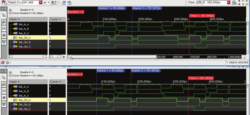
This feature applies a specified delay value to the input/output paths of all sequential UDPs in the design. The shift
register example in Figure 4 illustrates this.
-seq_udp_delay 50ps
When -seq_udp_delay is applied, it adds a delay from CK to Q (50ps in this example}. This causes
data to transition 50ps after CK and BCK, and causes the change in data to be seen by flop2 on the
next clock edge.
CK
D is assigned to Q/data D
after a 50ps delay
Q/data
Q/data and Qout go high at the same clock edge. BCK
Due to the delay, the change in Qout is reflected
at the next clock edge. That is, Qout changes to 0
at the second posedge instread of the first. Qout
0 300 700
-seq_udp_delay 50ps adds a delay At the next CK edge, Qout
of 50ps between CK and Q gets the value of Q
Buf1 BCK
CK delay 0ns
CK Q CK Qout
flop1 flop2
delay 50ps data D delay 50ps QN
D QN
Figure 4: Applying a Delay Value to I/O Paths of Sequential UPDs
Use the -seq _ udp _ delay option to set all of the delays to zero (as if you used the -delay _ mode _ zero
option) except for the sequential UDPs. The delay specified with -seq _ udp _ delay overrides any delay specified
for the sequential UDPs in the design that are in specify blocks, through SDF annotation, and so on. The option
also removes any timing checks associated with the sequential UDPs.
The delay _ specification argument can be a real number, or a real number followed by a time unit. The time
unit can be fs, ps, ns, or us. If no time unit is specified, ns is the default.
Examples
The following options assign a 10ns delay to all sequential UDP paths.
-seq _ udp _ delay 10
-seq _ udp _ delay 10ns
The following option assigns a 0.7ns delay to all sequential UDP paths.
-seq _ udp _ delay 0.7ns
The following option assigns a 5ps delay to all sequential UDP paths.
-seq _ udp _ delay 5ps
Figure 5 illustrates the effect of using -seq _ udp _ delay for the shift register example.
www.cadence.com 7Gate-Level Simulation Methodology
When -seq_udp_delay is applied, it adds a delay from
CK to Q (50ps in this example}. This causes data to
transition 50ps after CK and BCK, and causes the change
in data to be seen by flop2 on the next clock edge.
-seq_udp_delay 50ps adds a delay
of 50ps between CK and Q
BCK Value from D is clocked
Buf1 through flop1 on the first
CK delay 0ns CK edge and through flop2
on the second CK edge
CK Q CK Qout
flop1 flop2
delay 0ns data D QN
D QN
Figure 5: Using –seq_udp_delay for a Shift Register
Note that seq _ udp _ delay also does the following:
• Adds a delay to the sequential UDPs
• Implies -DELAY _ MODE ZERO
• Implies -NOSPECIFY
3. ADD_SEQ_DELAY delay_specification
As mentioned above, seq _ udp _ delay also internally implies delay _ mode _ zero and nospecify mode. In
case you are not interested in this mode, add _ seq _ delay can be used instead. This will add a non-zero delay to
the UDPs. The add _ seq _ delay option can also be applied for a specific instance.
For example:
-add _ seq _ delay top.dut _ top.u3 40ps
4. DELTA_SEQUDP_DELAY delay_specification
If you are not interested in adding UDP delays, delta _ sequdp _ delay can also be used. In most cases, just
adding a delta delay to the UDP is enough to avoid the race condition, and delta _ sequdp _ delay also adds less
overhead than a non-zero delay.
5. TIMING FILE
The delays can be controlled or even added through tfile.
5.1 Adding Unit or Zero Delays
Unit delays can also be controlled through the new tfile feature, which is available in release version 12.2 and
later. Using this feature, you can add unit delays in cells. This can be done at both the cell level and instance level.
To add unit delays at the cell level, the tfile syntax is:
CELLLIB L.C:V ADDUNIT //Add unit primitive delays
Example
CELLLIB worklib.sdffclrq _ f1 _ hd _ dh ADDUNIT //Adds unit delay to cell sdffclrq _ f1 _ hd _ dh
Similarly, to add a delay at the instance level, the tfile syntax is:
PATH .. ADDUNIT //Adds unit delay to instance INST2
www.cadence.com 8Gate-Level Simulation Methodology
Example
PATH tb.top1.clock _ div1.divide0 ADDUNIT //Adds unit delay to instance divide0
Overriding Default Cell Delays
The timing file feature also provides a mechanism to override the default delays specified at the cell level. As
mentioned in section 1.3.3 Sequential Circuits Have Unit Delays, in case #0 and #1 delays have already been added
in the cell library, and you can override these values using the ALLUNIT, UNIT, or ZERO keywords. This override
works only with the `delay _ mode _ distributed compilation directive. The following lines show this.
CELLIB L.C:V ALLUNIT //all non-zero and zero primitive delays will be changed to unit delay
CELLLIB L.C:V UNIT //all non-zero primitive delays will be changed to unit delay and zero
delay (#0) will remain as it is
CELLLIB L.C:V ZERO //all non-zero primitive delays will be changed to zero delay
Make Zero Delay
CELLLIB worklib.sdffclrq _ f1 _ hd _ dh zero
This feature also works at an instance level, as follows:
PATH .. zero //Adds zero delay to instance INST2
Similarly, you can use the unit or allunit keywords.
5.2 Adding Finite Delays to Instances
The user can add delays to a cell or an instance without changing the source code. On occasion, there are cases
with race conditions in the design but the user cannot modify the code. In order to fix such race conditions, user
can add delays through the tfile file without changing the source code.
The keyword is “-adddelay [precision]”
Without precision: Delays will be added based on the precision specified with timescale directive.
With precision: Absolute delays will be added.
Example of tfile file
PATH top.foo –adddelay 0 // This means add #0 precision delay at the output of instance top.foo
PATH top.foo –adddelay 1 // This means add #1 precision delay at the output of instance top.foo
CELLLIB mycell –adddelay 1 // This means add #1 precision delay at the output of all the instances of mycell
To add absolute delays
PATH top.foo –adddelay 10ps // This means add 10 ps delay at the output of instance top.foo
CELLLIB mycell –adddelay 12ps // This means add 12ps delay at the output of all the instances of mycell
Please note that this feature is available in release 14.2 and later.
www.cadence.com 9Gate-Level Simulation Methodology
2. Improving the Performance of Gate-Level Simulation with Timing
2.1 Timing Checks
Timing checks have a significant impact on performance, so it is recommended that you disable timing checks if
they are not required. Timing checks can also be enabled partially, only for required blocks, by passing a timing file
to Incisive Enterprise Simulator. The following sections present features that can help you control timing checks.
2.1.1 Use of the –NOTImingchecks Option
The NOTImingchecks option prevents the execution of timing checks. This option turns off both Verilog and accel-
erated VITAL timing checks.
Please Note: The -notimingchecks option turns off all timing checks. Because the timing checks have been
turned off, any calculation of delays that would normally occur because of negative limits specified in the timing
checks is disabled. If your design requires that these delays be calculated in order for the design to simulate
correctly, use the -ntcnotchks option mentioned below instead.
2.1.2 Controlling Timing Through a tfile
You can turn off timing in specific parts of a Verilog design by using a timing file, which you specify on the
command line with the -tfile option. The timing file can help you disable timing for selected portions of a design.
For example:
% ncelab -tfile myfile.tfile [other _ options] worklib.top:module
% irun -tfile myfile.tfile [other _ options] source _ files
If you are annotating with an SDF file, the design is annotated using the information in the SDF file, and then the
timing constructs that you specify in the timing file are removed from the specified instances.
Using a timing file does not cause any new SDF warnings or remove any timing warnings that you would get
without a timing file. However, there is one exception, as follows:
The connectivity test for register-driven interconnect delays happens much later than the normal interconnect
delays. Any warning that may have existed for that form of the interconnect will not be generated if that
interconnect has been removed by a timing file.
The timing specifications you can use in the timing file are listed in the following table:
Timing Specification Description
-iopath Disable module path delays.
+iopath Enable module path delays.
-prim Disable primitive delays. Sets any primitive delay within the specified
instance(s) to 0.
+prim Enable primitive delays within the specified instance(s).
-port Remove any port delays at the specified instance(s) or any interconnects
whose destination is contained by the instance. interconnect sources are not
affected by the -port construct.
+port Enable port delays at the specified instance(s) or any interconnects whose
destination is contained by the instance.
[list _ of _ tchecks] Remove the listed timing checks from the instance(s).
-tcheck
www.cadence.com 10Gate-Level Simulation Methodology
Timing Specification Description
[list _ of _ tchecks] Enable the listed timing checks in the instance(s).
+tcheck
If specific timing checks are not listed, all timing checks will be disabled or
enabled.
Examples:
// Disable all timing checks in top.foo
PATH top.foo –tcheck
// Disable $setup timing check in top.foo
PATH top.foo $setup -tcheck
// Disable $setup and $hold timing checks in top.foo
PATH top.foo $setup $hold -tcheck
-timing This is an alias for the four specifications shown above.
+timing
Example Timing File
The following listing shows an example timing file:
// Disable all timing checks in top.inst1
PATH top.inst1 -tcheck
/* Disable all timing checks in all scopes below top.inst1 except
for instance top.inst1.U3 */
PATH top.inst1... -tcheck
PATH top.inst1.U3 +tcheck
/* Disable $setup timing check for all instances under top.inst2,
except for top.inst2.U1. */
PATH top.inst2... $setup -tcheck
PATH top.inst2.U1 $setup +tcheck
// Disable $setup and $recrem timing checks for instance top.inst3
PATH top.inst3 $setup $recrem -tcheck
// Disable timing checks for all objects in the library mylib
CELLLIB mylib -tcheck
// Disable module path delays for all instances in the 2nd levels of hierarchy
PATH *.* -iopath
2.1.3 Use of the – NTCNOtchks Option
This option generates negative timing check (NTC) delays, but does not execute timing checks. The option is
available for Verilog designs only.
You can use the -notimingchecks option to turn off all timing checks in your design. However, if you have
negative timing checks in the design, this option also disables the generation of delayed internal signals, and you
may get the wrong simulation results if the design requires these delayed signals to function correctly. That is, if
you have negative timing checks, simulation results may be different when using -notimingchecks and without
-notimingchecks.
Use the -ntcnotchks option instead of the -notimingchecks option if you want the delayed signals to be
generated but want to turn off timing checks. This option removes the timing checks from the simulation after the
negative timing check (NTC) delays have been generated.
Controlling Timing Checks with the -NTCNOtchks Option Using a tfile
By default, all timing checks are disabled by the -ntcnotchks option. However, in case you are interested in the
timing violations for some portion of the design (typically the top block), the timing checks can be controlled using
the tfile timing file.
www.cadence.com 11Gate-Level Simulation Methodology
Please Note: This feature is available from release version 12.2 onwards.
The keyword ntcnotchks is available for use in the timing file. The keyword controls the -ntcnotchks option
at the instance level. Using the keyword enables the timing checks, and a delayed net will be generated for those
instances using the -ntcnotchks option.
Note: The – or + prefix is not required for the ntcnotchks option in the tfile. If ntcnotchks is present in the file,
it is always enabled.
Some example cases are presented here.
Case 1
Enable negative timing computation delays for all instances, with timing checks enabled for a particular
instance only.
Timing File Sample
//Enables Negative timing computation delays on the entire design but turns off timing
checks on all instances.
DEFAULT ntcnotchks
//Enables timing checks for a particular instance.
path top.u1 +tcheck
Case 2
Selectively enable negative timing check delays and timing checks.
Timing File Sample
//Disables timing checks & negative timing computation delays on the entire design
DEFAULT –tcheck
//Enables timing check & ntcnotchks for a particular instance.
path top.u1.u2 +tcheck
//Enables negative timing computations for a particular instance and disables tchecks
path top.u1.u3 ntcnotchks
path top.u1.u4 ntcnotchks
2.1.3 Controlling the Number of Timing Check Violations
The results of GLS are often not usable if timing violations are reported. Consequently, many designers do not
want to continue the simulation further if a timing violation is reported.
When timing violations are reported, you can cause the simulation to immediately exit by using the following
switch:
-max _ tchk _ errors
When this option is specified, the value of the number argument specifies the maximum number of allowable
timing check violations before the simulation exits.
Please Note: This feature is available in release 12.2 and onwards.
2.1.4 Disabling Specific Timing Checks During Simulation
The tcheck command turns timing check messages and notifier updates on or off for a specified Verilog instance.
The specified Verilog instance can also be an instance of a Verilog module instantiated in VHDL.
Command syntax:
tcheck instance _ path -off | -on
www.cadence.com 12Gate-Level Simulation Methodology
2.1.5 Table - Disabling Timing Information
Keyword Specifies
-NOSPecify Disable timing information described in specify blocks and SDF annotation
-NOTImingchecks Do not execute timing checks.
-NONOtifier Ignore notifiers in timing checks
-NO _ TCHK _ msg Suppress the display of timing check messages, while allowing delays to be
calculated from the negative limits
-NTCNOtchks Generate negative timing check (NTC) delays, but do not execute timing
checks (in cases where you want the delayed signals to be generated but
want to turn off timing checks).
2.2 Removing Zero-Delay MIPDs, MITDs, and SITDs
You can improve performance by removing interconnect or port delays that have a value of 0 from the SDF file. The
SDF Annotator parses and interprets zero-delay timing information but does not annotate it. By removing the zero-
delay information from the SDF file, you eliminate unnecessary processing of this information.
Note: This performance improvement recommendation applies only to MIPDs, MITDs, and SITDs.
3. Improving Performance in Debugging Mode
3.1 Wave Dumping
Waveform dumping negatively impacts simulation performance, so it should be used only if required. If the
waveform dumping activity is high, you can use the parallel waveform mcdump feature of ncsim. Waveform dumps
inside cells/primitives should be turned off (using probe … -to_cells).
Enabling Multi-Process Waveform Dumping
If you are running the simulator on a machine with multiple CPUs, you can improve the performance of waveform
dumping, and decrease peak memory consumption, by using the -mcdump option (for example, ncsim -mcdump
or irun -mcdump). In multi-process mode, the simulator forks off a separate executable called ncdump, which
performs some of the processing for waveform dumping. The ncdump process runs in parallel on a separate CPU
until the main process exits. You can see a 5% to 2X performance improvement depending upon the number of
objects probed.
3.2 Access
By default, the simulator runs in a fast mode with minimal debugging capability. To access design objects and lines
of code during simulation, you must use ncelab command-line debug options. These options provide visibility into
different parts of a design, but disable several optimizations performed inside the simulator.
For example, Incisive Enterprise Simulator includes an optimization that prevents code that does not contribute in
any way to the output of the model from running. Because this dead code does not run, any runtime errors, such
as constraint errors or null access de-references, that would be generated by the code are not generated. Other
simulation differences (for example, with delta cycle-counts and active time points) can also occur. This dead
code optimization is turned off if you use the ncvlog -linedebug option, or if read access is turned on with the
ncelab -access +r option.
The following line shows the ncelab –access debug command and command-line options that provide additional
information and access to objects, but reduce simulator speed. Because these options slow down performance, you
should try to apply them selectively, rather than globally.
ncelab –access +[r][w][c]
r provides read access to objects
www.cadence.com 13Gate-Level Simulation Methodology
w gives write access to objects
c enables access to connectivity (load and driver) information
To apply global access to the design, the following command can be used for read, write, and connectivity access:
% ncelab -access +rwc options top _ level _ module
Try to specify only the type(s) of access required for your debugging purposes. In general:
• Read (r) access is required for waveform dumping and for code coverage.
• Write (w) access is required for modifying values through PLI or Tcl.
• Connectivity (c) access is required for querying drivers and loads in C or Tcl, and for features like tracing signals
in the SimVision Trace Signals sidebar. In regression mode, connectivity access must be always turned off.
For example, if the only reason you need access is to save waveform data, use ncelab -access +r.
To maximize performance, consider using an access file with the ncelab -afile option instead of specifying global
access using the -access option. Any performance improvement is proportional to the amount of access that is
reduced. The maximum improvement from specifying -access rwc to using no access can be >2X. Even removing
connectivity (c) access can result in a 20-30% improvement. The typical gain of fine-tuning access in large environ-
ments is 15-40%
You can also write an afile to increase performance at the gate level.
Sample afile:
DEFAULT +rw
CELLINST –rwc
Note: A new switch –nocellaccess is also available in release 12.1 and later to turn off cell access.
Multiple Snapshots for Access
You can also maintain two snapshots—one with more or global access for debug mode, and the other with limited
or no access, for regressions. For performance, you can always use the snapshot with limited or no access and, in
the case of debugging, use the global access snapshot.
4. Other Useful Incisive Enterprise Simulator Gate-Level Simulation Features
4.1 Initialization of Variables
The -NCInitialize option provides you with a convenient way to initialize Verilog variables in the design when
you invoke the simulator, instead of writing code in an initial block, using Tcl deposit commands at time zero,
or writing a VPI application to do the initialization. This option works for Verilog designs only, and you can enable
the initialization of all Verilog variables to a specified value. To initialize Verilog variables, you use -ncinitialize
with both the ncelab and the ncsim commands as follows:
• Use ncelab -ncinitialize to enable the initialization of Verilog variables.
• Use ncsim –ncinitialize to set the value to which the variables are to be initialized when you invoke the
simulator.
For example:
% ncvlog test.v
% ncelab -ncinitialize worklib.top // Enable initialization
% ncsim -ncinitialize 0 worklib top // Initialize all variables to 0
When you invoke the simulator, all variables can be initialized to 0, 1, x, or z. For example, the following line
initializes all variables to 0:
ncsim -ncinitialize 0
www.cadence.com 14Gate-Level Simulation Methodology
Different variables can be initialized to 0, 1, x, or z randomly using rand:n, where n is a 32-bit integer used as a
randomization seed. For example:
ncsim -ncinitialize rand:56
Different variables can be initialized to 0 or 1 randomly using rand _ 2state:n. For example:
ncsim -ncinitialize rand _ 2state:56
See ncsim -ncinitialize in Cadence Help for details.
Note: You can also enable initialization by specifying global write access to all simulation objects with the -access
+w option. However, this option provides both read and write access to all simulation objects in the design, which
can negatively affect performance. The -ncinitialize option provides read and write access only to Verilog
variables.
5. Improving Elaboration Performance Using Multi-Snapshot Incremental
Elaboration (MSIE)
Incremental elaboration technology can be used in any case where turn-around time (time for newer versions to
simulate) is an overriding concern. In an SoC environment, there can be multiple IP used and newer revisions might
come in at different intervals in the verification process. MSIE technology can help the designer save build time and
start gate-level simulations sooner.
Comp/Elab
IP1
Simulate Comp/Elab
IP2
Simulate
… Comp/Elab
IPn
Simulate
Analyze / Debug / Fix Analyze / Debug / Fix Analyze / Debug / Fix
SoC Timeline
Comp/Elab Simulate
IP1 IPn
SoC
IP2
Analyze / Debug / Fix
Analyze / Debug / Fix
Figure 6: SoC Verification with Multiple IPs
MSIE can be applied as shown in the figure below, where there are multiple IP cores in an SoC top module. The
different primary snapshots can be created for each IP and top, and the testbench environment can be in the
incremental portion. Even in the case where a complete elaboration is required at once, all the primaries can be
built in parallel and, finally, the incremental portion can be built, including all primaries. This saves a lot of elabo-
ration time.
www.cadence.com 15Gate-Level Simulation Methodology
Incremental Top Level
Snampshot
SoC Top Verification Env.
IP1 (Inst 1) IP2 (Inst 2) IP3 (Inst 3) Test-Specific Shared
VE VE
IP1 Hierarchy IP2 Hierarchy IP3 Hierarchy
irun top.v -primname \
Primary Primary Primary -ip2 -primname ip2 \
Snapshot Snapshot Snapshot -primname ip3
irun -ip1.v \ irun -ip2.v \ irun -ip3.v \ All primaries can be
-mkprimsnap \ -mkprimsnap \ -mkprimsnap \
built in parallel
-snapshot ip1 -snapshot ip2 -snapshot ip3
Figure 7. MSIE with Multiple Primaries and Top, TB as Part of Incremental
MSIE Use Model
Apply to GLS with and without timing (SDF) —The technology can be directly applied and design partitioning can
be done as shown in the figure above.
MSIE can also be applied for DFT-style tests (serial or parallel scan). If the tests are set up so that each test has
a separate top-level HDL file containing the patterns (which is somewhat common), then building the DUT as a
primary snapshot with the SDF file, and then making the incremental snapshot the test+DUT, works very well.
Please note that for with timing (SDF), auto portioning of SDF is available in release 14.2 and later.
6. Accelerating Gate Level Simulations
The Cadence Palladium ® XP platform accepts design descriptions in both synthesizable RTL and gate-level repre-
sentations or mixed abstractions equally well. Gate-level designs are compiled using the UXE compiler targeting all
verification modes, including simulation acceleration and in-circuit emulation with minimal to no compromise on
capacity or speed. Generally speaking, as design sizes increase (or the number of objects to simulate increase), the
performance of a simulator subsides whilst the performance of the Palladium XP platform remains fairly constant
thereby achieving relatively higher verification speeds. For simulation acceleration, speed-ups of 100x or higher are
typical, whereas for in-circuit emulation, speed-ups of 10,000x or higher are achievable, reaching MHz speeds. For
large designs where the simulation speeds for gate-level designs are in the range of 1 to 10Hz, simulation accel-
eration can be as high as 10,000x, and in-circuit emulation could be as high as 100,000x over the GLS.
With the Palladium XP platform, gate level designs can be used for both pre-silicon verification and post-silicon
validation. Users can validate gate-level netlists synthesized by standard synthesis tools targeting silicon vendor
libraries, including DFT and scan overlay structures. Gate level netlists can also be used to identify and analyze peak
and average power at sub-system and system level.
Because timing cannot be enabled in the Palladium platform, it is ideal for verifying the functionality of a gate-level
netlist with zero-delay mode.
6.1 Gate-Level Simulation with Timing Using Palladium Platform and Software Simulator
Gate-level timing simulations for large SoCs have long runtimes as they have complex timing checks, and it can
take several days just for chip initialization. In addition to the long runtime, the other key challenge is debug of GLS
environment given that the turnaround time increases significantly with each iteration.
www.cadence.com 16Gate-Level Simulation Methodology
From a functional verification perspective, the timing checks/annotation during the initialization/ configuration
phase is of no significance/interest for most designs. So a unique (patent-pending) concept of Simulation-
Acceleration methodology/flow with sdf can be used where the sdf annotation is honored when the run is in
software simulator and without timing when the run is on the emulator.
The solution works by leveraging the hot-swap feature of the Palladium XP emulator. To expand on hot-swap, it is
a capability of the Palladium Simulation-Acceleration solution, which allows the design to be swapped between the
simulator (Incisive Enterprise Simulator) and emulator (Palladium). The design can be swapped into the emulator for
high performance and swapped out of the emulator and run in software simulator for debug.
With this methodology, the netlist simulations can be run with high performance on hardware by swapping the
design into the emulator for the complete initialization/configuration phase. Then, swapping out of the emulator
and running the rest of the test in the software simulator honoring the sdf, i.e., timing simulation. This helps the
SoC netlist configuration to run much faster.
Figure 8 depicts the netlist simulation runtime, where the initialization phase is in the time-consuming phase. We
therefore run the functional simulation during this time in the emulator without any timing. Then, we swap out of
the emulator to run the timing simulation with sdf in the software simulator.
Begin Test with
Start Initiation Sequence
SDF Annotation
Simultation Acceleration Flow
Swap into the PxP
DUT
DUT + TB Execute chip initiation
Sequence in Hardware
Swap into the Simulator
Figure 8. Palladium Hot-Swap Feature
This new concept and methodology can be used in any gate-level simulations with SDF timing, who have long
runtime challenges in design configuration/initialization of the chip as compared to real function simulation.
Please Note: Cadence has applied for a patent for this flow.
A Methodology for Improving Gate-Level Simulation
This section shows some methodologies that can help you reduce overall GLS verification time and make the
process more effective.
1. Effectively Use Static Tools Before Starting Gate-Level Simulation
Using static tools like linting and static timing analysis (STA) tools can effectively reduce the gate-level verification
time.
1.1 Linting Tool
It is recommended that you use static linting tools such as the Cadence HDL Analysis and Lint (HAL) tool before
starting zero-delay simulations. This can help you identify the issues or potential areas that can lead to unnecessary
issues in gate-level simulation.
www.cadence.com 17Gate-Level Simulation Methodology
Since simulation runs at gate level can take a lot of time, and based on the issues reported by the linting tools,
updates can be done in the gate-level environment up front, rather than waiting for long gate-level simulations
to complete and then fixing the issues. Some of the potential issues that can be identified by linting tools are as
follows:
• Detecting zero-delay loops
• Identifying possible design areas that can lead to race conditions
If race issues are detected, you can use the techniques listed in section 1.3 Handling Zero-Delay Race Conditions to
fix them.
1.2 Static Timing Analysis Tool
Static timing analysis tool information and reports can be used to start gate-level simulations with timing early in
the design cycle. The information from STA reports can help you run meaningful gate-level simulations with timing,
by focusing on the design areas that have met the timing requirements. Also, you should temporarily fix timing for
other portions of the design that require changes or updates for timing closure.
Some techniques that can be used for this are presented in this section.
1.2.1 Reducing Gate-Level Timing Simulation Errors and Debug Effort Based on STA Tool
Reports, Even If Timing Closure Is Incomplete for Some Parts of the Design
Since GLS runs much slower than simulations without timing, starting GLS timing verification early can be helpful.
However, this can lead to a lot of unnecessary effort in debugging the issues that are already reported by STA tools
like Cadence Encounter Timing System, as the design is still in the process of timing closure. As the timing issues
that have been reported by STA tools require fixes to the design, using the SDF from this phase directly in the
simulation will show failures in the simulation as well.
The designer can temporarily fix these violations in SDF through STA tools and start GLS in parallel. And at the
same time, timing issues in the design can be fixed by the timing closure team. This technique can help you:
• Reduce GLS errors based on STA (Encounter Timing System reports)
• Improve the design cycle/debug time during GLS:
–– You can focus on gate-level issues rather than known STA (Encounter Timing System) errors
–– Debugging and fixing issues in parallel during design phase:
»» STA (Encounter Timing System) timing violations
»» GLS (other than Encounter Timing System errors)
–– Running functionally correct GLS by ignoring Encounter Timing System errors
The following section gives an overview of the typical STA GLS flow and also describes techniques to temporarily
fix setup and hold violations.
Static Timing Analysis and Gate-Level Simulation Flow
The following figure illustrates an overview of a typical STA tool, such as Cadence Encounter Timing System and a
gate-level simulator, such as Incisive Enterprise Simulator.
www.cadence.com 18Gate-Level Simulation Methodology
Gate-Level Netlist
STA FLOW SIMULATOR FLOW
STA Tool Generates SDF with no
Violation Report timing issue
STA Tool generates Check for GLS Timing
timing report and SDF errors in SIM
report
Generates SDF
SDF ERRORS
No No
Yes SIM PASS
Fix the design Yes
issue and validate
it in STA again Designers Work
on Real Simulation can start
Design Fix only once complete Design Tape Out
STA is clean
Figure 9: Typical Static Timing Analysis Tool and Gate-Level Simulator
Handling STA Setup Violations
This technique can help designers temporarily fix setup timing violations reported by STA tools so that they do not
appear in the GLS. Consider the following simple example for a setup violation shown in Figure 10:
Setup Violation Example
Data In Data Out
FF1 Comb. Logic
D2 Failing FF2
Clock
Comb Logic Example
G5 Input to FF2.D2
FF1 Data Out
G1
G6 G4
G3
B
G2
C
End Point Slack (ns) Cause
Top/core/ctrl/FF2/D2 -0.56 Violated
Figure 10: Setup Violation
Here, a setup violation is reported at FF2 and the slack is -0.56. The sample combinational logic is also shown in
the figure. If the SDF is generated by an STA tool (in this case, Encounter Timing System) directly, then it will not
only report timing violations during GLS, but there will also potentially be a functionality mismatch, as the data for
D2 might not get latched at FF2 at the next clock cycle. This might impact the functionality of other parts of the
design as well.
www.cadence.com 19Gate-Level Simulation Methodology
Since this is a known issue and requires a fix in the combinational logic from FF1 to FF2, the GLS can temporarily
ignore this path, or the timing needs to be temporarily fixed. This can be done in the STA tool itself by setting a
few gate delays to zero and compensating for the slack. Once the slack is compensated for, then the SDF can be
generated and used by the GLS.
To help you understand this approach in detail, the following table shows the delays for each gate.
Gate Delay (ns) Cumulative Delay (ns)
G1 0.32 0.32
G2 0.25 0.57
G3 0.4 0.97
G4 0.35 1.32
G5 0.28 1.60
G6 0.33 1.99
Referring to Figure 10, within Encounter Timing System, starting from node FF2.D2, a traversal is done and the
slack at each node is checked. Looking at the table above, it can be seen that setting delays for G1 and G2 to zero
will compensate the slack of -0.56.
Similarly, all the setup violations can be temporarily fixed. STA can be run again on the modified timing to check if
there are any new violations added by assigning zero delays to the gates.
This approach can be helpful only when the violations reported by STA tools are limited in number and are present
only in some small part of the design. Using this approach will not work in cases where there are a lot of viola-
tions, and where they affect almost the complete design, as it would change the timing information in the SDF file
completely and make the simulation very optimistic.
Adding Negative Delays in SDF (Limited Cases)
The effects of the above case can also be mitigated by adding negative delays in the STA environment at gate G1,
if the negative delay value in the above example is less than or equal to the G1 delay (which is 0.32ns). This feature
of adjusting negative delays by the simulator is available only in the Incisive 13.2 release and onwards. This new
feature in Incisive Enterprise Simulator can only adjust delays for one level. If the delays cannot be adjusted for
more than level 1, the remaining negative values are set to zero. By default, the elaborator zeros out all negative
delays and issues a warning. To enable negative interconnect and module path delay adjustments, run the elabo-
rator with the -negdelay option (ncelab -negdelay or irun -negdelay). For example:
% ncvlog -messages test.v
% ncelab -messages tb -negdelay
or
% irun test.v -negdelay
Use the -neg _ verbose option (ncelab -neg _ verbose or irun -neg _ verbose) to print out the negative
delay adjustments and save them to the default log file, as shown:
% irun test.v -negdelay -neg _ verbose
...
file: test.v
...
Elaborating the design hierarchy:
Top level design units:
tb
...
Building instance-specific data structures.
Processing Negative Interconnect Delays...
www.cadence.com 20Gate-Level Simulation Methodology
Adjusting driver of net tb.out1...
Driver delay adjusted successfully...
Adjusting driver of net tb.out3...
Driver delay adjusted successfully...
Number of negative interconnect delays adjusted successfully: 2
2 Negative interconnect delays have been adjusted successfully.
...
Writing initial simulation snapshot: worklib.tb:v
Adjustment Rules for Negative Delays
Incisive Enterprise Simulator now supports negative delays on single output gates without the need to zero their
values. When enabling negative delay adjustments, the adjustments are applied in the following sequence:
1. Other interconnect delays at the port
2. Driver delays at the input
3. Load delays at the output
Note: When comparing the negative delay values to the total delays in a design, adjustments to negative delay
values will introduce inconsistencies with the delays specified in the SDF file and may affect elaborator perfor-
mance.
Please Note: For this approach Cadence is evaluating different designs to test corner scenarios and would like to
partner with design teams to review and deploy it. Contact your field AE if you are interested.
Handling STA Hold Violations
Hold violations are similar to set-up violations, as shown in Figure 11:
Hold
Violations
Data In Data Out
FF1 Comb. Logic
D2 Failing FF2
Clock
End Point Slack (ns) Cause
Top/core/ctrl/FF2/D2 -0.50 Violated
Figure 11: Hold Violation
A hold violation is reported at FF2 and the slack is -0.50. In order to temporarily fix the issue, an extra interconnect
delay of 0.5ns can be added at D2.
The following are the advantages, assumptions, and limitations for this flow.
Advantages
• Encounter Timing System violations will not appear in the GLS
• Improvements in design cycle time, as the designer can focus on GLS issues, other than issues reported by
Encounter Timing System
• Adding 0 delays for gates can improve GLS performance
Assumptions
• Most of the design is STA clean and has limited known violations
www.cadence.com 21Gate-Level Simulation Methodology
• Adding 0 delays will not add other STA timing errors
• Needs to be checked by re-running STA
Limitations
• New errors added by the above updates might not get corrected.
Generating and Using Smart SDF with Timing Abstractions Running Timing Simulations
STA tools have a capability for doing hierarchical timing analysis and generating SDF hierarchically. This feature is
included in STA tools because flat STA for a complete chip takes a lot of time.
Typically, there are IP cores in, or in portions of, the design that are re-used across different SoCs and are already
silicon-proven. Turning on complete timing for an SoC enables timing of internal cells of all the blocks and IP cores,
leading to a lot of redundant simulation overhead. Currently, the designer can turn off the timing of the complete
IP/module using the tool features, but this adds optimism at the SoC level since the delay at output ports of the IP
become zero. Also, the timing checks at the input pins of the IP are ignored.
IP that is timing-clean and integrated at the SoC level, if run with full timing enabled, requires timing for all flops
and combination logic for accurate timing results. Since the IP is already timing-clean, the only set of timing issues
that can come are at the SoC level, or at the integration of the IP, as shown in Figure 12.
SoC TOP IP
TOPIN1 TOPOUT1
IN1 OUT1
Comb. Logic 1
TOPIN2 FF1
Comb. IN2 FF1 Comb. FF2 Comb. FF3 Comb. FF4 OUT2 Comb.
FF4
TOPOUT2
Logic 1 Logic 2 Logic 3 Logic 4 Logic 4
CLK
CLK
TOPIN3 FF2 Comb. IN3
Comb. Logic 5 FF5 Comb. Logic 6
OUT3 Comb.
FF3
TOPOUT3
Logic 2 Logic 3
Potential timing issues at SoC integration
Figure 12:
The following types of timing models can be used to generate SDF for gate-level simulation:
• Interface logic models
• Extracted timing models
Please Note: For this approach Cadence is evaluating different designs to test corner scenarios and would like to
partner with design teams to review and deploy it. Contact your field AE if you are interested.
www.cadence.com 22Gate-Level Simulation Methodology
2. Interface Logic Models
An interface logic timing model (ILM) has partial timing of the block that includes the timing at boundary logic
only, but hides most of the internal register-to-register logic.
Consider the simple example shown in Figure 13.
IN1 OUT1
Comb. Logic 1
IN2 FF1 Comb. FF2 Comb. FF3 Comb. FF4 OUT2
Logic 2 Logic 3 Logic 4
CLK
IN3 FF5 OUT3
Comb. Logic 5 Comb. Logic 6
Figure 13: Full Timing Model Example Design
Flop-to-flop internal paths are not required, as they do not affect the interface path timing and we are interested in
the interface path timing only. In the figure below, the timing of internal gates is set to zero (marked by grey box).
IN1 OUT1
Comb. Logic 1
IN2 FF1 Comb. FF2 Comb. FF3 Comb. FF4 OUT2
Logic 2 Logic 3 Logic 4
Remove timing for these gates
CLK
IN3 FF5 OUT3
Comb. Logic 5 Comb. Logic 6
Figure 14: Interface Logic Model
2.1 Advantages of Using Interface Logic Models
The advantages of using interface logic models include:
• Good performance improvements, both in STA and GLS, since only a partial design is used
• High accuracy as interface logic and interface cells are preserved
Please Note: This is a patented flow (beta version) and is available in Cadence’s Tempus™ Timing Signoff Solution
to dump abstracted interface timing models for running effective GLS. Cadence would like to partner with design
teams to try and deploy this flow. Contact your field AE if you are interested.
www.cadence.com 23You can also read