INTEGRATING FUZZY-LOGIC DECISION SUPPORT WITH A BRIDGE INFORMATION MANAGEMENT SYSTEM (BRIMS) AT THE CONCEPTUAL STAGE OF BRIDGE DESIGN
←
→
Page content transcription
If your browser does not render page correctly, please read the page content below
www.itcon.org - Journal of Information Technology in Construction - ISSN 1874-4753

INTEGRATING FUZZY-LOGIC DECISION SUPPORT WITH A BRIDGE
INFORMATION MANAGEMENT SYSTEM (BRIMS) AT THE
CONCEPTUAL STAGE OF BRIDGE DESIGN
SUBMITTED: August 2017
REVISED: April 2018
PUBLISHED: May 2018 at https://www.itcon.org/2018/5
EDITOR: Turk Ž.

Nizar Markiz,
Ph.D. Candidate, Department of Civil Engineering, University of Ottawa
Address: 161 Louis Pasteur Pvt., Ottawa, ON, Canada, K1N 6N5
Email:nmark086@uottawa.ca

Ahmad Jrade,
Associate Professor, Department of Civil Engineering, University of Ottawa
Address: 161 Louis Pasteur Pvt., Ottawa, ON, Canada, K1N 6N5
Email:ajrade@uottawa.ca

SUMMARY: In recent years, infrastructure restoration has been backlogged with complex factors that have
captured the attention of municipal and federal authorities in North America and Europe. The subjective nature of
evaluating bridge conditions and bridge deterioration is one of the main factors that influences bridge maintenance,
repair, and replacement (MR&R) decisions. This study presents a stochastic fuzzy logic decision support integrated
with a bridge information management system (BrIMS) to forecast bridge deteriorations and prioritize
maintenance, repair, and replacement (MR&R) decisions at the conceptual design stage. The proposed system
considers numerous factors that influence the prioritization of bridge MR&R decision making including complex
time-dependent gamma shock models. A parametric analysis is conducted in order to quantify the degree of
accuracy of the system. Implementation of the system platform demonstrated the viability of integrating BrIMS
with fuzzy-logic deterioration forecast techniques at the conceptual stage of bridge design. The proposed system
is validated through a case study and found to be in agreement with actual bridge deterioration results with a
percentage difference of approximately 10 - 15 %. Besides that, the integrated platform may be utilized as a
forecasting tool that is capable of predicting and prioritizing MR&R decisions to components for diverse bridge
design alternatives.

KEYWORDS: Fuzzy-logic, Decision Support, Deterioration Forecast, Bridge Information Model, Bridge
Information Management System

REFERENCE: Nizar Markiz, Ahmad Jrade (2018). Integrating fuzzy-logic decision support with a bridge
information management system (BrIMS) at the conceptual stage of bridge design. Journal of Information
Technology in Construction (ITcon), Vol. 23, pg. 92-121, http://www.itcon.org/2018/5

COPYRIGHT: © 2018 The author(s). This is an open access article distributed under the terms of the Creative
Commons Attribution 4.0 International (https://creativecommons.org/licenses/by/4.0/),
which permits unrestricted use, distribution, and reproduction in any medium, provided
the original work is properly cited.

                                                                              ITcon Vol. 23 (2018), Markiz & Jrade, pg. 92
1. INTRODUCTION
Typically, forecasting bridge infrastructure deterioration from distinct condition assessments and statistics is a
challenging task. Due to the highly complex and erratic nature of infrastructure data, deterministic bridge
deterioration models are quite often not applicable. Temporal reliability analysis “hazard functions,” such as
Markov chains, Bayesian networks, and gamma models, have been developed for bridge and storm sewer systems.
Predicting bridge deterioration conditions is the main constituent of infrastructure asset management techniques.
Furthermore, a decision support system based on fuzzy-logic theory that assists asset managers in making
appropriate MR&R decisions is vital (Wang et al., 2015). Bridge performance indicators should be based on
bridge beneficiaries’ perceptions of technical parameters. Integrating these indicators with stochastic time-
dependent modeling of bridge deteriorations is important for planning and prioritizing MR&R activities. These
activities may include inspection, sampling, preventative and maintenance operations. Based on the
aforementioned, a time-dependent prediction of the overall bridge deteriorations necessitates the development of
a thorough, reliable, and user-friendly fuzzy-logic decision support system.

1.1 Problem Definition
Nowadays, most bridge information management methodologies are strictly based on life cycle analyses offset by
available funds and budget constraints. Repair costs, in many situations, have proven to exceed annual or semi-
annual preventive maintenance costs (Liang et al., 2002). Most bridge stakeholders are reluctant to pay for
preventive maintenance, which appears to be of no benefit or which bridge asset managers have found from
experience to be unsuccessful in preventing a bridge structure from deteriorating.
In an attempt to overcome this shortcoming, this study is intended to demonstrate the viability of stretching bridge
information models to capture the conceptual design of a bridge while applying sensitivity analyses to identify the
most sensitive elements and subsequently to forecast bridge elemental deteriorations. Furthermore, it is assumed
that integrating a fuzzy logic decision support system with BrIMS and deterioration forecast for bridges is possible
only if its objectives are kept simple, focused, and organized. Therefore, basic straightforward bridge information
management (BrIMS) processes have been researched, recalled, and analyzed. According to Bentley bridge
solutions, the eight processes of BrIMS are: (1) bridge type selection; (2) 3D CAD model; (3) technical analysis;
(4) planning for construction; (5) production; (6) phases of construction; (7) maintenance; and (8) remediation
(Peters, 2009). Extending research published by Wang and Elhag (2008) and Cheng and Hoang (2012) that
proposed the integration of BrIMS with fuzzy systems to prioritize MR&R solutions for deteriorating bridges,
authors of this study introduce the idea of a fuzzy-logic decision support framework integrated with gamma shock
modelling for forecasting bridge deteriorations. The main advantage of such integration underlies the benefit of
capturing economical preventative maintenance routes and making strategic MR&R decisions at the conceptual
design stage.
Whilst several attempts have been made at modeling the deterioration of bridge infrastructures, practical
developments were recorded recently, where researchers employed the gamma stochastic process effectively to
temporal deteriorations and subsequently implemented into MR&R decision support systems. Furthermore, earlier
research work had not considered the integration of decision support systems with gamma shock models at the
conceptual design stage. In contrast, researchers had focused more on improvement factors for enhancing bridge
maintenance and information management techniques.
In this study, the following processes; i) bridge type selection; ii) 3D CAD model; iii) technical analysis; and iv)
maintenance and remediation are selected for the development and integration of gamma shock models BrIMS at
the conceptual design stage. The proposed system integrates quality functions for maintenance, repair, and
replacement (MR&R) alternatives with a Gaussian probabilistic matrix factorization. The resulting system
produces competitive priority ratings that eliminate ambiguities in bridge life cycle evaluation. Hence, the
proposed integrated information management system becomes a new approach to informing downstream processes
of bridge projects at the conceptual design stage.

                                                                                  ITcon Vol. 23 (2018), Jung et al., pg. 93
1.2 Research Objectives
The integrated approach presented herein may be utilized to plan the maintenance and to monitor the deterioration
of bridges and then to prioritize the maintenance, repair, and replacement alternatives; (i.e., inspection, sampling,
preventative, and maintenance operations). This integration technique is a rational approach that justifies most
“ineffective” spending by bridge stakeholders, since it considerably reduces subjectivity in quantifying bridge
deterioration. Moreover, the integration not only contributes to the reliability of a particular bridge element but
also to the reliability of the collected data and the probability of occurrence of deterioration benchmarks such as
corrosion and elemental degradations.
The main objective of this study, then, is to develop fuzzy logic decision support system using complex quality
functions and a gamma stochastic deterioration model that is based on the integration of probabilistic models in
an attempt to improve the effectiveness of bridge information management systems. Towards that goal, a wider
insight into the integration of a decision support system can assist bridge asset managers in proposing a strategic
solution to deteriorating bridge infrastructures.

1.3 Literature Review
Highway and transportation authorities have often relied upon deterministic deterioration curves for predicting
bridge maintenance programs. In past years, bridge infrastructure management systems have been modeled using
traditional Markov chain models. In the past three decades, inconsistent MR&R decisions for bridges and road
infrastructures have necessitated the evolution of further investigative studies in the modeling of bridge
deteriorations in parallel with developing reliable decision support solutions (Lounis, 2000).
According to earlier studies conducted by Golabi et al. (1993) and Hawk (1999), incremental degradation of bridge
components were designed by a static Markov chain model process in which accumulating deficiencies following
a stress cycle were assumed to depend on original conditions and duration of the cyclic stress loading only.
However, a study conducted by Madanat et al. (1997) confirmed that most bridge deterioration models were not
static and proposed descriptive variables that traditional Markov models must take into account to develop more
realistic models. Furthermore, Lounis (2000) restated the capability of Markov models in predicting the remaining
service life of a bridge at any time based on existing deterioration conditions.
Recent bridge information management systems have implemented Markov chains deterioration models which is
considered a major step forward towards incorporating stochastic-natured deterioration models. Moreover, several
bridge maintenance aspects and corresponding bridge asset visual inspection standards and procedures endorsed
the implementation of the Markov chain model which is known to possess restrictive assumptions. Although
traditional Markov chain models are proven practical and relatively simple to develop, they do possess limitations
especially at comprehensive project phases and are considered not sufficient for analyzing critical structures when
it comes to safety matters. The most important limitation, however, is the deployment of elemental condition crisp
rating systems based on vague performance indicators mainly influenced by the scale of subjectivity involved in
the visual inspection and not explicitly related to qualitative and quantitative parameters such as material
properties, stress-strain conditions, and structural behavior. Proceedings and evolutions that tailored the Markov
chain approach in bridge information management systems were provided in a study published by Frangopol et al.
(2001). In a later study later, Lounis and Madanat (2002) presented a two-level decision support system that
amalgamates stochastic deterioration models to enhance efficacy of bridge maintenance management systems. The
first level management is based on Markov models that pin points perilously damaged structures and predicts
short- and long-term deterioration and essential maintenance at a bridge-level and network- level. While the second
level management is based on mechanistic models that target considerably deteriorated bridge structures classified
from the first level management and assess their integrity, serviceability, and maintenance.
In an attempt to overcome Markov chain model limitations, reliability-based deterioration models that are based
on gamma shock models have been researched and recalled.. One study conducted by Pandey and Van Noortwijk
(2004) investigated a gamma model for temporal structural reliability and presented a relative assessment of
random variable deterioration models based on the first order reliability methods and temporal stochastic modeling
based on the gamma process. In their paper, the authors employed a stochastic model to count for both sampling
and time-dependent variances allied with a structural system deterioration process. A detailed comparison of
lifetime probability and cumulative density functions as well as survival curves between random variable and

                                                                                   ITcon Vol. 23 (2018), Jung et al., pg. 94
gamma process mechanisms were presented. It was concluded that the random variable model overestimates
probability of remaining life time of a particular structure in the long-run and gamma model provides more
reasonable estimates of life times which shall enhance the implementation of such stochastic deterioration models
more often in structure reliability analysis. In another study, Van Noortwijk et al. (2005) examined a gamma
process model for temporal structural reliability and presented a combined computational method comprising both
deterioration resistance and variable load modeled as a stochastic gamma process. It is concluded that the time at
which the deteriorating resistance falls below the fluctuation load cumulative distribution function can be
formulated as a functional equation which could be solved numerically by applying a series of integration and
partial derivations to simulate deterioration paths of the generalized gamma process. It was also found that the
proposed method contributes to the ‘well-fit’ of structural monotonic aging peaks-over-threshold distributions with
extreme value figures. Furthermore, Van Noortwijk et al. (2007) examined gamma processes and peaks-over-
threshold distributions for time-dependent reliability. In their paper, a comprehensive discussion on the evaluation
of structural reliability was presented where a methodology that integrated two stochastic processes originating
from a Poisson process for obtaining the temporal reliability of a particular structural component was proposed.
Another study conducted by Edirisinghe et al. (2013) presented the application of gamma process for stochastic
deterioration prediction of building elements derived from discrete condition data obtained from the Victorian
local government infrastructure asset database. The focus of their study was geared to develop a complex and more
reliable deterioration prediction system for managing their building assets. Gamma process probability and
cumulative density functions were derived and plotted in addition to building elements predicted temporal
deterioration. At the end, the authors concluded with the capability of the proposed gamma process deterioration
model for forecasting deterioration of building elements with time by incorporating building condition and
deterioration highly scattered data. Moreover, Reddy and Ramudu (2013) analyzed a numerical arithmetic-
geometric maintenance model for deteriorating system subject to a random environment. Their main goal was to
develop a replacement model for a particular deteriorating system in a random environment while utilizing an
arithmetic-geometric approach that maximizes long-run anticipated payoff within a cycle time. System
replacement average cost rate versus the replacement policy were obtained and plotted where the peak of the curves
explicitly indicates an optimal replacement policy. At the end, the authors concluded that by varying the parameters
of the developed model, the optimal number of failure only impacts the long-run anticipated payoff cost per cycle
time.
In summary, there have been substantial efforts to apply a gamma model to the perseverance of bridge structures.
Although advancements in deterioration modeling have influenced bridge MR&R solutions, arguments for its
application to time-dependent incremental degradations of bridge elements still exist. This study presents the
proposal of a reliability-based deterioration model based on the deployment of complex quality functions
originating from the house of quality (HOQ) model. The proposed decision support system is based on quantitative
and qualitative fuzzy logic scorings that take into account technical, functional, and safety parameters. Moreover,
such systems are powerful in the manner that they are capable of analyzing single or multiple complicated bridge
elements of a highway bridge that possess diverse failure modes.

2. SYSTEM ARCHITECTURE
The proposed methodology comprises an innovative bridge information management system (BrIMS) based on a
framework that is capable of integrating bridge gamma stochastic deterioration modeling with a fuzzy-logic
decision support system. The framework is developed by deploying complex quality functions derived from bridge
beneficiary-driven parameters and symmetrical triangular fuzzy numbers (STFN’s) to capitulate bridge evaluation
ambiguities. Furthermore, the proposed system possesses a unique aspect of BrIMS by incorporating diverse
bridge MR&R solutions into a multi-criteria decision making approach (MCDM) to derive competitive priority
ratings. A schematic view of the interrelations among the 3D computer-aided design (CAD) solutions with the
developed bridge deterioration forecast system is illustrated in Fig. 1.

                                                                                  ITcon Vol. 23 (2018), Jung et al., pg. 95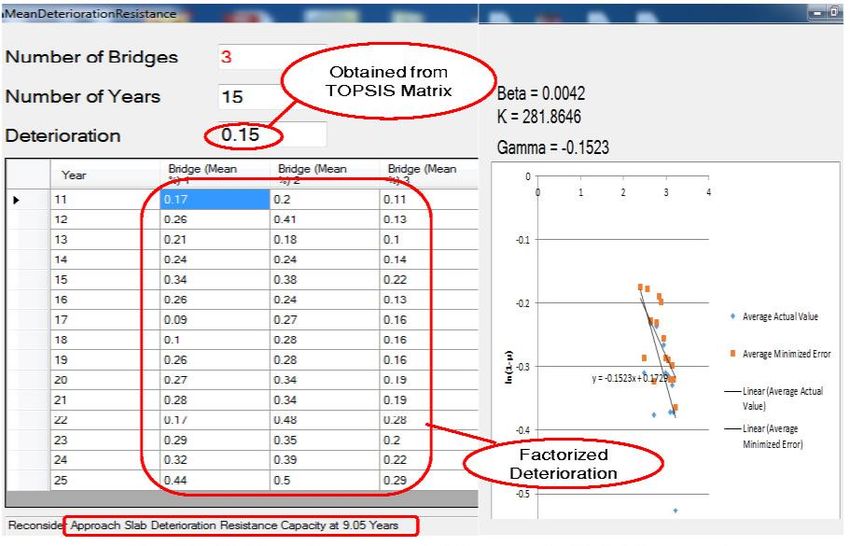
FIG. 1: Proposed System Architecture
As illustrated in Fig. 1, it is important to note that the proposed integrated system is part of an integrated
preliminary fuzzy-logic decision support system developed earlier by the authors of this study. The following two
modules:
Module 1 – Conceptual Bridge Design
Module 4 – Deterioration Forecast
are an integral part of this study whereas the highlighted items that correspond to the following three modules:
Module 2 – Fleet Selection
Module 3 – Preliminary Cost Estimation
Module 5 – Bridge Line of Balance
are not part of this study. The proposed system is developed in an object-oriented .NET framework and undertaken
by completing the following six main steps:
1) Data collection of bridge-user-driven parameters.
2) Implementation of a decision support system that assists the user in making MR&R decisions.
3) Development of complex quality functions to evaluate bridge users’ relative perception of
bridge components.
4) Deployment of a numerical model to evaluate bridge MR&R ratings.
5) Development of a mean deterioration resistance regression fit where MR&R rankings are determined.
6) Optimizing and prioritizing maintenance, repair, and replacement alternatives.
At first, the user inputs importance ratings on bridge components. Following bridge user’s assessment on the
importance of bridge components on bridge design alternatives, importance perception ratings are determined.
Afterwards, a bridge users’ competitive matrix is developed, where the probability distribution and corresponding
measure of entropy of bridge components is determined. Once completed, the user proceeds with inputting a set
of improvement goals that represent the user’s required improvement in performance of bridge components.
Following the input of goals, QFD and TOPSIS analyses are undertaken in order to develop priority rankings of
bridge components. Afterwards, the user is guided to the HOWs scoring input form, which represents bridge users’
importance ratings on bridge maintenance, repair, and replacement alternatives (MR&R) based on the output of
ITcon Vol. 23 (2018), Jung et al., pg. 96
QFD and TOPSIS analyses on bridge components, Following bridge user’s assessment on the importance of bridge
components on MR&R alternatives, importance perception ratings are obtained. Afterwards, a bridge users’
competitive matrix is developed, where the probability distribution and corresponding measure of entropy along
with competitive ranking of bridge components is determined. Afterwards, the user inputs the year digit and
corresponding mean deterioration percentages such that a regression analysis along with the quality of fit
methodology is deployed. Once completed, the developed system provide the user a recommendation statement to
reconsider the performance of a bridge component in order to enhance its deterioration resistance capacity, which
represents a component’s remaining service life. Fig. 2 summarizes the deterioration forecast module process
flowchart.

FIG. 2: Deterioration Forecast Module Process Flowchart

As illustrated in Fig. 2, the developed module is implemented in an object-oriented .NET framework and
undertaken by completing the following five main steps:
    1) Data collection of bridge type and geometric selection imported from Module 1.
    2) Implementation of a decision support system that assists the user in making MR&R decisions.
    3) Development of complex quality functions to evaluate bridge users’ relative perception of bridge
         components.
    4) Deployment of a numerical model to evaluate bridge MR&R ratings.
    5) Prioritizing maintenance, repair, and replacement (MR&R) alternatives.

The flow of geometric information for diverse bridge types and resistance deterioration predictions begins at fuzzy
logic scorings and ends at the forecasting of bridge component deterioration based on its cost recovery period.
Throughout the process, the deployment of the technique of preference by similarity to ideal solution (TOPSIS),
a multi-criteria analytical approach utilized for the selection of the MR&R alternative based on a specified list of
parameters is undertaken. The MR&R are identified based on performance condition assessments of bridges in
operational stages and grouped into three main categories as follows; Category (I) is a ‘Maintenance’ category that
includes the maintenance of a bridge component for an expected extent ranging between 15% to 45% and
comprising the decisions; ‘Maintenance: S1.M15’, ‘Maintenance: S2.M30’, and ‘Maintenance: S3.M45’; Category
(II) is a ‘Repair’ category that includes the repair of a bridge component for an expected extent of deterioration
ranging between 45% to 75% and comprising the decision; ‘Repair: S4.REPA45’, ‘Repair: S5.REPA60’, and
‘Repair: S6.REPA75’; Category (III) is a ‘Replacement’ category that includes the replacement of a bridge
component for an expected extent of deterioration ranging between 75% to 100% and comprising the decisions;
‘Replacement: S7.REPL75’, ‘Replacement: S8.REPL90’, and ‘Replacement: S9.REPL100’. The MR&R
alternatives are defined as cost representatives of a bridge component. For instance, a maintenance ‘M15’
alternative represents ‘15%’of a bridge component’s estimated cost.

                                                                                  ITcon Vol. 23 (2018), Jung et al., pg. 97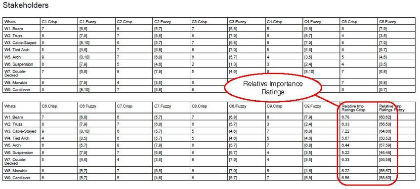
2.1 Fuzzy Logic Decision Support System
Due to the scarcity of bridge deterioration data, it is necessary to develop a fuzzy logic scoring system in order to
assist bridge stakeholders and designers in predicting bridge deterioration at conceptual design stages. Otayek et
al. (2012) have studied the integration of a decision support system based on a proposed machine technique as part
of artificial intelligence and neural networks (NN). In their study, the authors recommend continuous and further
development in decision support systems in an attempt to assist bridge designers in predicting bridge deteriorations
at conceptual phases. On the other hand, Malekly et al. (2010) have proposed a methodology of implementing a
quality function deployment (QFD) technique and a technique of preference by similarity to ideal solution
(TOPSIS). Their methodology is integrated in a novel oriented approach while overcoming interoperability issues
among the disperse databases. Furthermore, Tee et al. (1988) studied the viability of developing a numerical
approach based on fuzzy set rules such that the degree of subjectivity involved in evaluating bridge deterioration
was treated systematically and was incorporated into a systematic knowledge-based system. Liang et al. (2002)
proposed grey and regression models for predicting the remaining service life of existing reinforced concrete
bridges. In their study, the fuzzy logic concept was introduced as a methodology for evaluating the extent of
deterioration of existing bridge structures. Zhao and Chen (2002) proposed a fuzzy logic system for bridge
designers to help to predict bridge deteriorations based on factors incorporated at the initial design phase. Sasmal
et al. (2006) recalled earlier studies using fuzzy logic theory and stated that those methodologies were either much
too simple or too complex so that key support requires considerable time.
These studies; however, overlooked key issues pertaining to membership functions and other parameters, such as
priority vectors and mappings, which are fundamental for bridge condition assessments. Therefore, the authors of
the present study propose an integrated system for deterioration evaluations of bridges, based on fuzzy
mathematics integrated with an eigen-vector technique and priority ratings. In this study, the proposed system is
anticipated to be of novelty to BrIMS integrated technologies and possess a great advantage over the diverse
deterioration forecast algorithms, prototypes, and systems presently used in the bridge construction industry by
including a fuzzy logic decision support system based on quality functions deployment (QFD) and the technique
of order preference by similarity to ideal solution (TOPSIS). As a result, competitive priority ratings of bridge
components alternatives are produced rather than completely including or excluding alternative solutions at the
conceptual design stage. Fig. 3 illustrates a high-level process of the fuzzy logic decision support system integrated
with the BrIMS.
As shown in Fig. 3, the proposed system includes a fuzzy logic decision support that extracts information from the
3D BrIM tool via a DLL-invoked API method that automatically recalls the parametric enriched object-oriented
model. For instance, the system provides the user with an option to develop an information module by utilizing
the fuzzy logic scoring system in order to determine the bridge type based on the deployment of the QFD and
TOPSIS processes; otherwise, the application automatically extracts data from the BrIM model and presents
nominations and recommendations of selected bridge type based on technical and functional spans and
geotechnical attributes. Furthermore, the system is hard-coded to extract all necessary information from the
assigned model by exporting BrIM input databases via the Industry Foundation Classes (IFC) file format, which
reduces loss of information during file transmission. After that, the system is objectively developed for bridges
such that capturing of data displayed in the calling software is conducted by utilizing BrIM objects. Finally, bridge
element attributes are recalled and organized via a DLL-invoked programming language and incorporated into the
SQLite database server.

                                                                                    ITcon Vol. 23 (2018), Jung et al., pg. 98
FIG. 3: Deterioration Forecast Module Process Flowchart

2.1.1 Quality Functions
Conceptual bridge design is found to be significantly influenced by each of the following nine main components:
(1) approach slab ‘C1’; (2) deck slab ‘C2’; (3) expansion joint ‘C3’; (4) parapet ‘C4’; (5) girder ‘C5’; (6) bearings
‘C6’; (7) abutment ‘C7’; (8) pier ‘C8’; and (9) foundation ‘C9’. Selection of the components is based on critical
factors that bridge designers rely upon and bridge users’ perception on the importance of components. Hence, a 9-
point symmetrical triangular fuzzy logic numbers (STFN) ranging from one to nine, with one being very low and
nine being very high, is adopted for assisting the decision maker in predicting bridge users perception pursuant to
the main nine bridge components listed above. The scoring system comprises crisp and fuzzy measures when
uncertainty arises.
Where for instance, [0,2] indicates the range of fuzziness of the crisp score ‘1’. Similarly, [8,10] represents the
range of fuzziness of the crisp score ‘9’. Afterwards, bridge users are identified and categorized as follows: (i)
stakeholders/government; (ii) designers/engineers; (iii) contractors/builders; and (iv) public/residents. Also, the
following nine common bridge types ‘alternatives’ are identified and incorporated into the database platform for
QFD analyses: (1) beam bridges ‘W1’; (2) truss bridges ‘W2’; (3) cable-stayed bridges ‘W3’; (4) tied-arch bridges
‘W4’; (5) arch bridges ‘W5’; (6) suspension bridges ‘W6’; (7) double-decked bridges ‘W7’; (8) movable bridges
‘W8’; and (9) cantilever bridges ‘W9’. The adopted QFD analytical technology utilized for the selection of bridge
type is presented in Fig. 4.

                                                                                   ITcon Vol. 23 (2018), Jung et al., pg. 99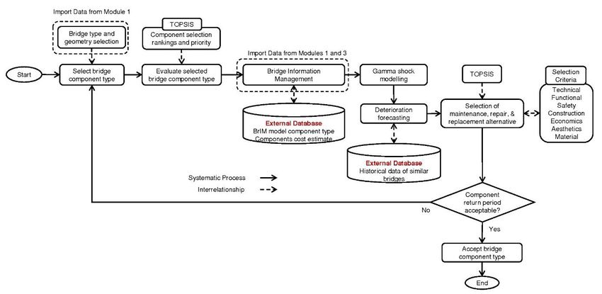
FIG. 4: Quality Function Deployment Process Flow
Upon completion of user scorings on the nine bridge components, perception on relative importance ratings of the
components is determined. In this study, Chan and Wu (2005) numerical methodology is deployed due to its
efficiency, systematic characteristics, and ease of use in competitive analysis of bridge components selection. Crisp
and measure forms of expected relative importance ratings are obtained in accordance with Chan and Wu (2005)
equations (1) and (2):
( g m1 g m 2 g m3 g m 4 g m5 g m6 g m7 g m8 g m9 )
g mk (1)
9
~ ( g~m1 g~m 2 g~m3 g~m 4 g~m5 g~m6 g~m7 g~m8 g~m9 )
g mk (2)
9
Where; g mk is a bridge user relative importance perception on a component in ‘crisp’ form, k is a bridge user,
~
g mk is a bridge user relative importance perception on a component in ‘fuzzy’ form. In other words, g mk is the
average “integer” crisp scoring value of a bridge user on the relative importance of each of the components and
g~mk is the average “integer” fuzzy scoring value of a bridge user on the relative importance of each of the
components. Following the determination of relative importance ratings, bridge users competitive comparison
matrix analysis is developed as per Chan and Wu (2005) equations (3) and (4):
X xmk 9x9 (3)
( xm11 xm12 xm13 xm14 )
xmlk (4)
4
Where; X is the bridge users comparison matrix, xmk is a bridge user assessment on Cm , xmlk is a bridge user
assessment of a bridge alternative on Cm , and Cm is a bridge component. Afterwards, the probability distribution
of each Cm on bridge alternatives is calculated using Chan and Wu (2005) equation (5):
ITcon Vol. 23 (2018), Jung et al., pg. 100
xmk
pmk (5)
xm
Where; pmk is the probability distribution of Cm on bridge alternatives, xmk is a bridge user assessment on Cm
‘result obtained from equation (4)’, and xm is the total of bridge users assessment of all bridge alternatives on
each of Cm . Following the determination of probability distribution of C m , its measure of entropy, which is a
quantification of the expected value of a system with uncertainty in random variables, may be obtained using Chan
and Wu (2005) equations (6) and (7):
9
E (Cm ) 9 pmk ln( pmk ) (6)
l 1
1
9 (7)
ln(9)
Where; E (Cm ) is the measure of entropy by a discrete probability distribution for Cm , 9 is the normalization
factor that guarantees 0 E ( p1 , p2 ,....., pL ) 1 , pmk is the probability distribution of C m for the diverse
bridge alternatives. Higher entropy or ( p1 , p2 ,..... pL ) implies smaller variances and lesser information in a
probability distribution p L . At the end, bridge alternatives’ weights on each of the nine C m is calculated based
on Chan and Wu (2005) equation (8):
E (C m )
em 9
(8)
E (C
m 1
m )
Where; em is the importance weight of bridge component, Cm , and E (Cm ) is the measure of entropy by a
discrete probability distribution for C m . This complex quality function deployment mechanism of assigning
priorities to competing alternatives is directly related to information theory concept of entropy. Once completed,
a set of improving goals strategy on each of the bridge components to enhance the bridge alternative deterioration
resistance performance is defined. The performance goals on the bridge components are identified based on the 9-
point STFN scale as per Chan and Wu (2005) equation (9):
i (i1 , i2 , i3 , i4 , i5 , i6 , i7 , i8 , i9 ) (9)
Where; i is the improvement goal set. It is important to note that the improvement goals must be higher than the
initial performance rating of a bridge component, C m for a bridge alternative, Wm . This implies that in case the
initial rating of a component for a particular bridge alternative is high, the goal set must be higher to maintain its
rating and enhance the competition amongst bridge alternatives. Otherwise, if the initial rating is lesser, then the
improvement goal is set to improve the performance of the same and enhance its importance weight. Once
improvement goals are set, an improvement ratio is calculated as per Chan and Wu (2005) equation (10):
im
rm (10)
xmk
Where; rm is the improvement ratio, im is the improvement goal set, and xmk is a bridge user assessment on Cm
‘result obtained from equation (4)’. The competitive rating for a bridge component, C m , in ‘crisp’ form is obtained
as per Chan and Wu (2005) equation (11):
f m im * g m * em (11)
ITcon Vol. 23 (2018), Jung et al., pg. 101Where; f m is the competitive rating, im is the improvement goal set, g m is a bridge user relative importance
e
perception on a component in ‘crisp’ form, and m is the importance weight. The final importance rating for a
C
bridge component, m , in ‘fuzzy’ form is obtained as per Chan and Wu (2005) equation (12):
~
f m im * g~m * em (12)
~
im is the improvement goal set, g~m is a bridge user relative
Where; f m is the competitive rating in ‘fuzzy’ form,
importance perception on a component in ‘fuzzy’ form, and em is the importance weight. Once completed,
technical measures to expected maintenance, repair, and replacement (MR&R) decisions to the deterioration of
bridge components are grouped into three main categories as illustrated in Table 1.
TABLE 1: Maintenance, Repair, and Replacement Decisions Versus Extent of Deterioration (%)
Extent of Deterioration Category Category Category
(%) I II III
15 √ - -
30 √ - -
45 √ √ -
60 - √ -
75 - √ √
90 - - √
100 - - √
As illustrated in Table 1, category (I) is a ‘Maintenance’ category that comprises maintenance of bridge component
for an expected extent ranging between 15% to 45% and comprising the decisions; ‘Maintenance: S1.M15’,
‘Maintenance: S2.M30’, and ‘Maintenance: S3.M45’; category (II) is a ‘Repair’ category that comprises repair of
bridge component for an expected extent of deterioration ranging between 45% to 75% and comprising the
decision; ‘Repair: S4.REPA45’, ‘Repair: S5.REPA60’, and ‘Repair: S6.REPA75’; category (III) is a ‘Replacement’
category that comprises replacement of bridge component for an expected extent of deterioration ranging between
75% to 100% and comprising the decisions; ‘Replacement: S7.REPL75’, ‘Replacement: S8.REPL90’, and
‘Replacement: S9.REPL100’. It is important to note that the proposed categories and extent of deterioration is for
illustrative purposes and can be customized dependent upon the bridge location and the regional weather forecast.
Similar to the determination of competitive comparison matrix analysis on bridge components, user comparison
matrix analysis on technical measures for expected deterioration in ‘crisp’ and ‘fuzzy’ forms respectively are
determined as per Chan and Wu (2005) equations (13) and (14):
R rmn 10x9 (13)
R ~
rmn 10x9
~
(14)
Where; R is the comparison matrix on technical measures, rmn is a bridge user technical measure assessment on
Cm in ‘crisp’ form, ~
rmn is a bridge user technical measure assessment on Cm in ‘fuzzy’ form, and Cm is a bridge
component. Hence, the technical rating for a measure, t mn , on a bridge component, C m in ‘crisp’ form is obtained
as per Chan and Wu (2005) equation (15):
9
tmn f m * rmn where; n 1, 2, ....10 (15)
m1
ITcon Vol. 23 (2018), Jung et al., pg. 102Where; t mn is the technical rating on a measure in ‘crisp’ form, f m is the competitive rating ‘result obtained from
r C
equation 11’ in ‘crisp’ form, and mn is a bridge user technical measure assessment on m in ‘crisp’ form. The
r C
technical rating for a measure, mn , on a bridge component, m in ‘fuzzy form is obtained as per Chan and Wu
(2005) equation (16):
9
~
tmn f m * ~
~
rmn where; n 1, 2, ....10 (16)
m1
~ is the technical rating on a measure in ‘fuzzy’ form, ~ is the competitive rating ‘result obtained
Where; tmn fm
~
from equation 12’ in ‘fuzzy’ form, and rmn is a bridge user technical measure assessment on Cm in ‘fuzzy’ form.
Afterwards, the probability distribution of each Cm on bridge deterioration technical measures is calculated using
Chan and Wu (2005) equation (17):
xmn
pmn (17)
xm
Where; pmn is the probability distribution of Cm on technical measure, xmn is a bridge user assessment on Cm
‘result obtained from equation (4)’, and xm is the total of bridge users assessment of all technical measure on each
of Cm . Following the determination of probability distribution of C m , its measure of entropy, which is a
quantification of the expected value of a system with uncertainty in random variables, may be obtained using Chan
and Wu (2005) equations (18) and (19):
10
E (Cm ) 10 pmn ln( pmn ) (18)
l 1
1
10 (19)
ln(10)
Where; E (Cm ) is the measure of entropy by a discrete probability distribution for Cm , 10 is the normalization
factor that guarantees 0 E ( p1 , p2 ,....., pL ) 1 , pmn is the probability distribution of C m for the diverse
technical measures. Higher entropy or ( p1 , p2 ,..... pL ) implies smaller variances and lesser information in a
probability distribution p L . At the end, bridge technical measure weights on each of the nine C m is calculated
based on Chan and Wu (2005) equation (20):
E (Cm )
et 9
(20)
E (C
m1
m )
Where; et is the importance weight of technical measure, and E (Cm ) is the measure of entropy by a discrete
probability distribution for C m .
2.2 Technique for Order of Preference by Similarity to Ideal Solution (TOPSIS)
Upon determination of technical measure weights, a multi-criteria decision making approach, TOPSIS, is
undertaken. This approach takes into account the following criteria: (i) qualitative benefit; (ii) quantitative benefit;
and (iii) cost criteria. As part of TOPSIS analysis, the following two most contradicting alternatives are surmised:
(a) ideal alternative in which the maximum gain from each of the criteria values is taken; and (b) negative ideal
alternative in which the maximum loss from each of the criteria values is taken. Towards the end, TOPSIS opts in
ITcon Vol. 23 (2018), Jung et al., pg. 103for the alternative that converges to the ideal solution and opts out from the negative ideal alternative. Prior to
undertaking the multi-criteria decision making approach, a TOPSIS matrix is created based on equation (21):
X xij (21)
Where; X is the bridge users comparison matrix; and xij is an “m x n” matrix; where, ‘m’ represents the technical
measures and ‘n’ represents the bridge components that display the score of bridge user ‘ i ’on bridge component
‘ j ’. TOPSIS analysis comprises the following consecutive five steps: (i) normalized decision matrix; (ii)
weighted normalized decision matrix; (iii) ideal and negative ideal solutions; (iv) bridge components separation
measures; and (v) relative closeness to ideal solution as shown in Fig. 5.
FIG. 5: TOPSIS Process Flow
In this study, Hwang et al. (1993) numerical methodology is deployed based on its direct applicability to ranking
bridge MR&R priorities and proven reliability. Generating the normalized decision matrix is intended to convert
various parametric dimensions into non-dimensional parameters to allow for contrasting among criteria using
Hwang et al. (1993) equation (22):
xij
rij (22)
x 2
ij
Where; rij is the normalized scoring value of bridge users on bridge components. Afterwards, the development of
a weighted decision matrix is obtained by multiplying the importance weights determined from equations (8) and
(20) by its corresponding column of the normalized decision matrix obtained from equation (22) through the
deployment of Hwang et al. (1993) equation (23):
vij wi rij where; wi em * et (23)
Where; vij is the weighted normalized element of the TOPSIS matrix, and wi is the final importance weight, et
is the importance weight of technical measure, and em is the importance weight of bridge component. Afterwards,
the ideal and negative ideal solutions are determined using Hwang et al. (1993) equations (24) and (25):
ITcon Vol. 23 (2018), Jung et al., pg. 104
A* v1 ,..., v j
* *
(24)
A v ,..., v
' ' '
1 j (25)
Where; A is the positive ideal solution; where v j max vij if j J ; minimum vij if
* *
j J ' ; A' is the
v j min vij if j J ; maximum vij if j J ' ; where J is the set of positive
'
negative ideal solution where
'
attributes or criteria; and J is the set of negative attributes or criteria. Afterwards, bridge competitors’ separation
measures from ideal and negative ideal solutions are calculated by using Hwang et al. (1993) equations (26) and
(27):
Si
*
(v j
*
vij ) 2
1/ 2
(26)
Si
'
(v j
'
vij ) 2 1/ 2
(27)
* '
Where; S i is the separation from the positive ideal solution; S i is the separation from the negative ideal solution;
and i is the number of bridge competitors. Finally, relative closeness to ideal solution is calculated by using
Hwang et al. (1993) equation (28):
'
Si
Ci
* *
; 0 < Ci < 1 (28)
Si Si
* '
*
Where; Ci is the relative closeness to positive ideal solution. The highest-ranked bridge component for MR&R
*
priorities is the one with a corresponding Ci closest to the value of unity ‘1’.
2.3 Gamma Deterioration Model
Typically, bridge deteriorations are mainly caused by chemical and/or physical mechanisms that significantly
affect infrastructure material characteristics and subsequent components. In this study, the deterioration of an aging
bridge infrastructure is typically modelled as a function of its resistance capacity. The deterioration function is
defined as per Noortwijk et al. (2007) in equation (29):
D(t ) Ro R(tk ) (29)
Where D(t ) is the deterioration function, Ro is the initial resistance, and R(t k ) is the resistance at time t k . The
deterioration function is assumed to be an ascending-order process with independent deterioration time intervals.
For instance, suppose a sequence of shock load effects occur at discrete times such that the overall bridge service
period is divided into independent time intervals. Hence, the resistance deterioration function, R(tk ) , at time t k ,
is represented as equations (30) and (31) from Wang et al. (2015):
R(tk ) Ro D(tk ) (30)
k
D(tk ) 1 Gi where; k 1, 2, ....n (31)
i 1
Where R(tk ) is the resistance deterioration function, Ro is the initial resistance; D(t k ) is the deterioration at
time t k ; and Gi ~ Ga( , ) denotes a gamma function with the shape parameter, , and the scale parameter,
. It is important to note that equation (30) is a descending-order process with a corresponding mean and variance
calculated as per Wang et al. (2015) in equations (32-a), (32-b), and (32-c):
ITcon Vol. 23 (2018), Jung et al., pg. 105k
D(t k ) 1 i (32-a)
i 1
k
2 D(t k ) 2 i where; k 1, 2, ....n (32-b)
i 1
*i (ti ti1 ) (32-c)
Where is the mean; D(t k ) is the deterioration at time t k ; 2 is the variance, *i is the deterioration
parameter; is the scale parameter; and is the rate of deterioration. It is important to note that the scale and
shape parameters presented herein are assigned as deterioration parameters of random variables and are determined
independently.
2.4 Determination of Deterioration Function
Typically, bridge element conditions are evaluated by conducting site inspections based on municipal and/or
national standards. These inspections contribute significantly towards the resistance deterioration condition of
bridge elements and reflect their existing state which may be predicted as a ratio of the existing deterioration
resistance to its initial resistance as per Wang et al. (2015), in equation (33):
Rk
D(t k ) (33)
Ro
Where D(t k ) is the deterioration function at time t k ; Rk is the current resistance deterioration function at time
t k ; and Ro is the initial resistance. The existing resistance deterioration function Rk , and the initial resistance
Ro , are typically estimated according to bridge design manuals and national code standards. Bridge deterioration
resistance is rarely assessed due to the high costs incurred, which implies that very little or no information on
existing bridge resistance is available. Hence, this study proposes a numerical method to estimate deterioration
parameters based on previous data of similar bridges.
2.4.1 Estimation of Deterioration Parameters
In order to estimate the deterioration parameters ( ) and ( ), the shape and scale deterioration function D(t k )
presented in equation (33) will be utilized to determine the deterioration of similar existing bridges k , with a
corresponding service life of t1 , t 2 ,....tk . By substitution, the deterioration function is presented as per Wang et
al. (2015) in equation (34):
1 D(t )i (ti ) where; i 1, 2, ....k (34)
Where D(ti ) is the deterioration at time ti ; and are the random shape and scale and deterioration
parameters, and is the rate of deterioration. By taking the logarithmic for both sides of equation (34), the
deterioration function is expressed as per Wang et al. (2015) in equation (35):
ln(1 D(t )i ) ln( ) ln(ti ) (35)
Now, the deterioration parameters and can be estimated graphically by utilizing a regression analysis of
previous similar bridges’ deterioration data; where the slope is the ratio of ln(1 D(t )i ) to ln(ti ) and the
y-intercept is . In equation (32-b), the variance does not account for the dynamic nature of the temporal
deterioration function. Hence, an average variance formulation is presented as per Wang et al. (2015) in equation
(36):
k k
ˆ 2 ˆ ti ( D(t )i Dˆ (ti )) 2
ˆ
where ; (36)
i 1 i 1
ITcon Vol. 23 (2018), Jung et al., pg. 106k
( D(t ) i Dˆ (t i )) 2
ˆ ˆ
ˆ i 1
and ˆ
k
ˆ
ˆ ˆ t k
ˆ
i 1
Where ˆ and ˆ are the estimated shape and scale deterioration parameters respectively; ̂ is the estimated rate
ˆ (t ) is the estimated deterioration at time ti .
of deterioration; D(ti ) is the deterioration at time ti ; and D i
3. SYSTEM IMPLEMENTATION AND VALIDATION
The implementation of the decision support system is undertaken in two main steps; i) perturbation; and ii) quality
evaluation. The algorithm is implemented as a probabilistic distribution function such that a random deterioration
variable, D , possesses a standard Gamma distribution of a distinguished shape parameter, , and scale parameter,
, defined as per Johnson et al. (1995) in equation (37):
1
x
x
f D ( x) e where; x, , and 0 (37)
( )
Where x is the deterioration parameter, is the shape parameter, is the scale parameter, and is the gamma
function defined as per Johnson et al. (1995) in equation (38):
( ) x 1e x dt (38)
0
In this study, a gamma model with shape and scale parameters greater than zero is assumed to be a continuous
stochastic model if the following conditions are satisfied: i) probability of D(0) 0 is unity; ii) D(t ) comprises
independent deterioration increments; and iii) increments follow a gamma function such that the mean and variance
are determined as per Johnson et al. (1995) in equation (39):
D(t ) and 2 D(t ) 2 (39)
Where is the mean, is the variance, is the shape parameter, and
2
is the scale parameter.
3.1 Quality of Fit
Although regression analysis is capable of modeling a data scatter, significant variance may be noticed in the
manner it represents the actual data value. Testing the quality of fit of a regression analysis trend line is typically
conducted by either of the two following procedures: 1) heuristic, where manual inspection is conducted in parallel
with an error minimization procedure; or 2) non-heuristic procedure, where hypothetical procedures such as the
Chi-square test are deployed. In order to ease the use of regression analysis, the manual inspection of trend line
fitting with an error minimization procedure is adopted since such fittings are automatically generated with
advanced modeling software available in the market. The procedure is based on adjusting the fitted trend line to
minimize the error. The sum (E) of the squares of differences between the actual and proposed trend line fit is then
minimized to obtain the magnitude of adjustment factor that results in the best fit with the actual data scatter. The
error minimization procedure is identified as per equation (40):
n
d act,i a d pro,i 2
Emin (40)
i 1 d act, i
Where Emin is the minimized error, i 1...n is the number of actual data scatters, d act,i is the actual data value
th
at the i location, d pro,i is the proposed data value at the i th location, and a is a scaling factor to be applied to
ITcon Vol. 23 (2018), Jung et al., pg. 107the proposed trend line. It is noted that the bracketed terms in equation (20) have been normalized with respect to
the average of actual data, d act, i as per equation (41):
1 n
d act,i d act,i
n i1
(41)
Towards the end, it is important to note that the proposed trend line fit contributes towards an accurate estimation
of the shape and scale deterioration parameters such that error tolerances are respected.
3.1.1 Probabilistic Matrix Factorization
As part of enhancing dataset quality, collaborative filtering algorithms to determine interrelationships amongst
deterioration parameters are investigated. The matrix factorization approach is found to be the most effective
amongst the examined techniques due to its latent feature in determining the underlying correlations amongst
independent variables. In this study, a probabilistic matrix factorization technique is deployed to predict
deterioration datasets of existing bridges while overcoming biased and over-fitted values. The model-based
approach is undertaken by the following four main processes: (1) singular value matrix decomposition (SVMD);
(2) data normalization; (3) factorization; and (4) regularization. Firstly, the matrix decomposition process is
deployed to predict resistance deterioration values, [ g (t )] , of a bridge component as per Takács et al. (2008),
in equation (42):
rˆij pi q j 1 pik qkj
T k
(42)
T
Where r̂ij is the predicted resistance deterioration; pi is the bridge preference factor vector; q j is the resistance
deterioration factor vector; pik is the bridge preference factor matrix; and qkj is the resistance deterioration factor
matrix such that the dot product of pik and qkj approximates the r̂ij . Afterwards, a gradient descent technique
T
is deployed in order to determine the bridge preference and resistance deterioration factor vectors pi and q j
respectively. The error between the predicted and actual resistance deterioration value to obtain a local minima of
each ‘bridge-resistance deterioration’ pair is determined as per Takács et al. (2008) as in equation (43):
e 2 ij (rij rˆij ) 2 (rij 1 pik qkj ) 2
k
(43)
Where; e 2 ij is the squared error difference; rij is the actual resistance deterioration; r̂ij is the predicted resistance
deterioration; pik is the bridge preference factor matrix; and qkj is the resistance deterioration factor matrix. It
is important to note that the squared error of the predicted and actual resistance deterioration data is implemented
in order to account for over- or under-estimated values.
3.1.2 Error Minimization
In order to minimize the error value, a modification to pik and qkj matrices is required to determine the value of
the gradient at its present state. Hence, a differentiation of equation (43) with respect to pik is deployed as per
Takács et al. (2008) in equation (44):
2
e ij 2(rij rˆij )(qkj ) 2eij qkj
pik
(44)
2
e ij 2(rij rˆij )( pik ) 2eij pik
qkj
Where e 2 ij is the squared error difference; eij is the error difference; rij is the actual resistance deterioration; r̂ij
is the predicted resistance deterioration; pik is the bridge preference factor matrix; and qkj is the resistance
ITcon Vol. 23 (2018), Jung et al., pg. 108deterioration factor matrix. Upon determination of the gradient descent value, the differentiation of equation (23)
is rearranged as per Takács et al. (2008) in equation (45):
2
p'ik pik e ij pik 2eij qkj
pik
(45)
2
q'kj qkj e ij qkj 2eij pik
qkj
Where p'ik is the differentiated bridge preference factor matrix; q'kj is the differentiated resistance deterioration
factor matrix; e 2 ij is the squared error difference; is the gradient descent rate factor; eij is the error difference;
pik is the bridge preference factor matrix; and qkj is the resistance deterioration factor matrix. It is important to
note that the factor in equation (45) is the tolerance value that defines the rate of gradient descent approaching
the minimum. In order to avoid excessive oscillations and bypassing the local minima, a modification factor ,
with a value of 0.0002 is assumed. In this study, the error minimization procedure is proposed for the bridge-
resistance deterioration pairs. For instance, let N be a finite ordered set of training data in the form of ( qkj ,
pik , r̂ij ), the error, eij , for each iterative dataset will be minimized when the connotations amongst the attributes
is learnt. Afterwards, the error minimization process is concluded when the iteratively determined error converges
to its minimum as per Takács et al. (2008) in equation (46):
E ( q (rij 1 pik qkj ) 2
k
(46)
kj , pi k ,rˆij )N
Where E is the minimized error value; qkj is the resistance deterioration factor; pik is the bridge preference
factor matrix; r̂ij is the predicted resistance deterioration; and rij is the actual resistance deterioration.
3.1.3 Regularization
In order to avoid dataset over-fitting, a regularization process is implemented by incorporating a parameter factor
, to regularize the magnitudes of the bridge-deterioration resistance factor vectors. Also, a regularization
parameter with a value of 0.02 is assumed in order to avoid large number approximations and achieve a better
approximation of the bridge deterioration resistance capacity. The squared-error difference between the predicted
and actual resistance deterioration value to obtain a local minima of each ‘bridge-resistance deterioration’ pair is
rearranged as per Takács et al. (2008) in equation (47):
e 2 ij (rij rˆij ) 2 (rij 1 pik qkj ) 2 (p
k k 2
qkj )
2
1 ik (47)
2
2
Where e ij is the squared error difference; rij is the actual resistance deterioration; and r̂ij is the predicted
resistance deterioration; pik is the bridge preference factor matrix; and qkj is the resistance deterioration factor
matrix. Upon determination of the squared error difference, the differentiation of the equation (43) is rearranged
as per Takács et al. (2008) in equation (48):
2
p'ik pik e ij pik (2eij qkj pik )
pik
(48)
2
q'kj qkj e ij qkj (2eij pik qkj )
qkj
ITcon Vol. 23 (2018), Jung et al., pg. 109Where p'ik is the differentiated bridge preference factor matrix; q'kj is the differentiated resistance deterioration
factor matrix; e 2 ij is the squared error difference; is the gradient descent rate factor; is the regularization
parameter; eij is the error difference; pik is the bridge preference factor matrix; and qkj is the resistance
deterioration factor matrix.
3.2 System Validation
To validate the workability of the proposed system, a case study of a bridge in Ottawa, Canada composed of a
concrete box-girder with a total span of 200 ft. supported with a central interior bent at 100 ft. is developed in
CSiBridge as illustrated in Fig. 6. The challenge underlying the system validation is to provide priority ranking to
MR&R decisions for the diverse bridge components.
FIG. 6: Conceptual Bridge Design Information Model
Prior to inputting project related data into BrIM tool, the following list summarizes main parametric design
assumptions: 1) Abutment: skewed at 15 degrees and supported at bottom girder only; 2) Pre-stressing: 4 nos. 5
in2 tendons with a 1,080 kips capacity each; 3) Interior bent: 3 nos. 5 ft square columns; 4) Deck: parabolic
variation ranging from 5-10 ft in nominal depth; 5) Pile cap: 3 nos. 13’ x 13’ x 4’; and 6) Pile: 9 nos. 14” dia. steel
pipe filled with concrete reinforced with 8 nos. of #9 reinforcement bars at each pile cap. It is important to note
that the aforementioned assumptions are made based on normal job conditions. However, if geographical
constraints are encountered, these factors may increase or decrease accordingly. For example, if the job terrain
encountered is rough, substructure concrete and pile design factors will increase and subsequently significantly
influence overall project cost. The systematic procedure of the integrated system is demonstrated in a step-by-step
process in Figs. 7 through 12 which present snapshots of the proposed system modules. Fig. 6 presents the
integrated deterioration gateway module.
ITcon Vol. 23 (2018), Jung et al., pg. 110You can also read