Aerodynamic optimization of pylons to improve rear wing performance using passive and active systems
←
→
Page content transcription
If your browser does not render page correctly, please read the page content below
Aerodynamic optimization of pylons
 to improve rear wing performance
 using passive and active systems
 Master’s thesis in Automotive engineering

 Avaneesh Upadhyaya
 Kaushik Nagaraja Rao

DEPARTMENT OF MECHANICS AND
MARITIME SCIENCES

CHALMERS UNIVERSITY OF TECHNOLOGY
Gothenburg, Sweden 2021
www.chalmers.se
MASTER’S THESIS IN AUTOMOTIVE ENGINEERING

Aerodynamic optimization of pylons to improve rear wing performance using
                       passive and active systems

                               AVANEESH UPADHYAYA
                              KAUSHIK NAGARAJA RAO

                       Department of Mechanics and Maritime Sciences
              Division of Vehicle Engineering and Autonomous Systems (VEAS)
                      CHALMERS UNIVERSITY OF TECHNOLOGY
                                 Göteborg, Sweden 2021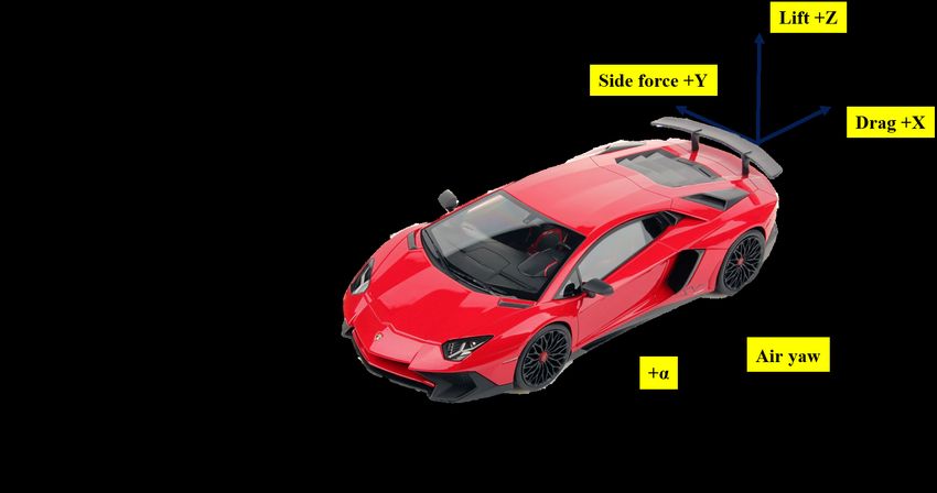
Aerodynamic optimization of pylons to improve rear wing performance using passive and active systems
AVANEESH UPADHYAYA
KAUSHIK NAGARAJA RAO

© AVANEESH UPADHYAYA, KAUSHIK NAGARAJA RAO, 2021

Master’s thesis 2021:15
Department of Mechanics and Maritime Sciences
Division of Vehicle Engineering and Autonomous Systems (VEAS)
Chalmers University of Technology
SE-412 96 Göteborg
Sweden
Telephone: +46 (0)31-772 1000

Supervisor: Magnus Urquhart, Department of Mechanics and Maritime Sciences
Supervisor: Ugo Riccio, Automobili Lamborghini S.p.A
Supervisor: Vincenzo Sepe, Automobili Lamborghini S.p.A
Examiner: Simone Sebben, Department of Mechanics and Maritime Sciences

Cover:
Aventador Superveloce[1]

Chalmers Reproservice
Göteborg, Sweden 2021
Aerodynamic optimization of pylons to improve rear wing performance using passive and active systems
Master’s thesis in Automotive Engineering
AVANEESH UPADHYAYA
KAUSHIK NAGARAJA RAO
Department of Mechanics and Maritime Sciences
Division of Vehicle Engineering and Autonomous Systems (VEAS)
Chalmers University of Technology

                                                Abstract
In collaboration with Automobili Lamborghini S.p.A, an aerodynamic investigation was carried out on a dual
pylon rear wing assembly to improve cornering stability of a car at high speeds. The pylon’s primary purpose
is to provide structural support to the wing. However, this project aimed at improving the performance
of Aventador SV’s rear wing using aerodynamically optimized pylons that not only boosted its downforce
generating capabilities, but also generated large side forces at higher yaw angles.

The project goals were fulfilled in two phases. The first phase involved development of pylon airfoils that would
keep the flow attached within a range of ±15 yaw angles, without augmenting the drag when compared to
NACA0010. A surrogate based model was used to generate these airfoils. 2D simulations were performed on
the airfoils along with passive and active systems to achieve attached flow around the pylons, thus, generating
more downforce by improving suction under the wing. Single slot approach was used to create passive slots that
improved flow on one side of the design at the expense of the other. The active flow control was implemented
in two ways, blowing and suction. Throughout this study, active blowing has held precedence due to energy
constraints. Three airfoils with better performance than NACA0010 at higher yaw angles were selected for
next phase.

In the second phase, airfoils from 2D study were used to carry out 3D simulations using RANS solver
on several wing and pylon combinations, without a car body, in a quest to find the optimum performing pylon.
A study was conducted to analyse the effect of different pylon positions, sizes, and profiles along with passive
and active systems on the air flow around the wing. With the profiles generated in 2D study, an improvement
in the performance of the wing was achieved at higher yaw angles. Wherever the flow detached over the pylon,
passive and active systems showed signs of improvement.

Keywords: Pylons, Rear Wing, Aerodynamics, Asymmetric Airfoil, Low Reynolds, Lift, Drag, CFD, Passive,
Active, STAR-CCM+

                                                        i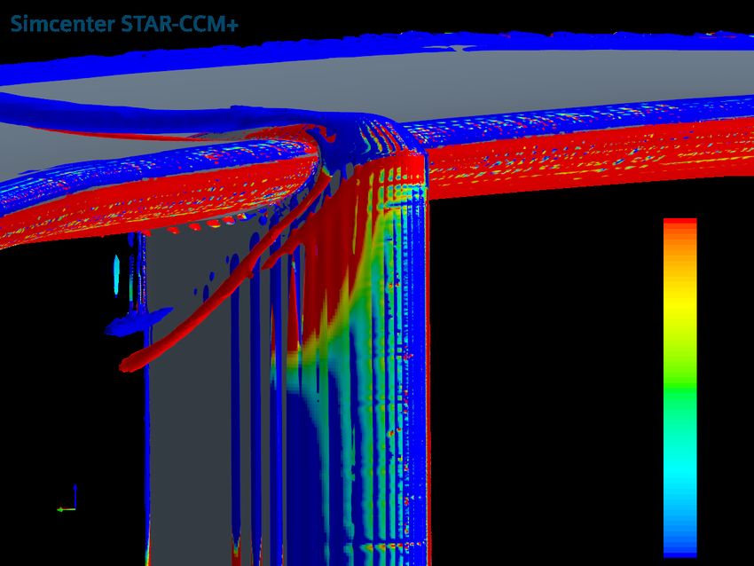
ii
Acknowledgements
We would like to express our utmost gratitude to our supervisor Magnus Urquhart at Chalmers for their
patient guidance and supervision throughout the thesis. The thesis would not have progressed as far as it
did without his useful and constructive recommendations. Thank you Magnus for generously devoting your
time to our questions. We would like to extend our gratitude towards our industry supervisors Ugo Riccio and
Vincenzo Sepe at Automobili Lamborghini S.p.A for their valuable critiques and insights to guide us in the right
direction. We appreciate the time and effort you invested in us and we thoroughly enjoyed working alongside
you. Completing this project would not have been possible without the kind support and encouragement
provided by our examiner Simone Sebben. Thank you for ensuring that this project proceeded without any
hurdles.

                                                       iii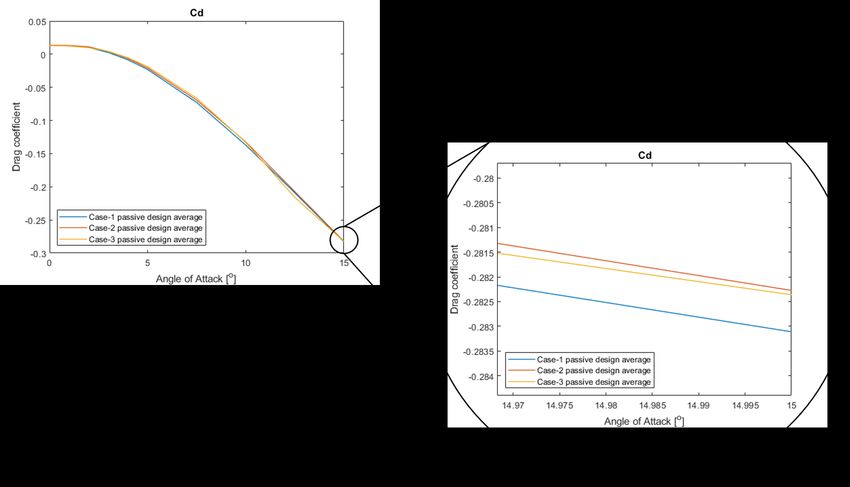
iv
Contents

Abstract                                                                                                                                                                                 i

Acknowledgements                                                                                                                                                                       iii

Contents                                                                                                                                                                                v

List of Figures                                                                                                                                                                        vii

List of Tables                                                                                                                                                                         ix

1 Introduction                                                                                                                                                                          1
1.1 Purpose . . . . . . . . . . . . . . . . . . . . . . . . . . . . . . . . . . . . . . . . . . . . . . . . . . .                                                                       2
1.2 Literature Study . . . . . . . . . . . . . . . . . . . . . . . . . . . . . . . . . . . . . . . . . . . . . .                                                                        2
1.3 Limitations . . . . . . . . . . . . . . . . . . . . . . . . . . . . . . . . . . . . . . . . . . . . . . . . .                                                                       4

2 Airfoil Study                                                                                                                                                                         5
2.1 Simulation Overview . . . . .     . . . . . . .    .   .   .   .   .   .   .   .   .   .   .   .   .   .   .   .   .   .   .   .   .   .   .   .   .   .   .   .   .   .   .   .    5
2.1.1 Coordinate System & Force       Coefficients     .   .   .   .   .   .   .   .   .   .   .   .   .   .   .   .   .   .   .   .   .   .   .   .   .   .   .   .   .   .   .   .    5
2.1.2 Solver and flow parameters      . . . . . . .    .   .   .   .   .   .   .   .   .   .   .   .   .   .   .   .   .   .   .   .   .   .   .   .   .   .   .   .   .   .   .   .    6
2.2 Mesh Study . . . . . . . . . .    . . . . . . .    .   .   .   .   .   .   .   .   .   .   .   .   .   .   .   .   .   .   .   .   .   .   .   .   .   .   .   .   .   .   .   .    6
2.3 Airfoil Optimization . . . . .    . . . . . . .    .   .   .   .   .   .   .   .   .   .   .   .   .   .   .   .   .   .   .   .   .   .   .   .   .   .   .   .   .   .   .   .    7
2.4 Passive and Active Systems .      . . . . . . .    .   .   .   .   .   .   .   .   .   .   .   .   .   .   .   .   .   .   .   .   .   .   .   .   .   .   .   .   .   .   .   .    8
2.4.1 Passive system . . . . . . .    . . . . . . .    .   .   .   .   .   .   .   .   .   .   .   .   .   .   .   .   .   .   .   .   .   .   .   .   .   .   .   .   .   .   .   .    8
2.4.2 Active system . . . . . . . .   . . . . . . .    .   .   .   .   .   .   .   .   .   .   .   .   .   .   .   .   .   .   .   .   .   .   .   .   .   .   .   .   .   .   .   .    8

3 Results & Discussion - Airfoil Study                                                                                                                                                 10
3.1 Generated Airfoils . . . . . . . . . . . .     .   .   .   .   .   .   .   .   .   .   .   .   .   .   .   .   .   .   .   .   .   .   .   .   .   .   .   .   .   .   .   .   .   10
3.2 NACA0010 . . . . . . . . . . . . . . . .       .   .   .   .   .   .   .   .   .   .   .   .   .   .   .   .   .   .   .   .   .   .   .   .   .   .   .   .   .   .   .   .   .   12
3.2.1 NACA0010: Active . . . . . . . . . .         .   .   .   .   .   .   .   .   .   .   .   .   .   .   .   .   .   .   .   .   .   .   .   .   .   .   .   .   .   .   .   .   .   13
3.3 Case 1 . . . . . . . . . . . . . . . . . . .   .   .   .   .   .   .   .   .   .   .   .   .   .   .   .   .   .   .   .   .   .   .   .   .   .   .   .   .   .   .   .   .   .   14
3.3.1 Case 1: Passive . . . . . . . . . . . . .    .   .   .   .   .   .   .   .   .   .   .   .   .   .   .   .   .   .   .   .   .   .   .   .   .   .   .   .   .   .   .   .   .   14
3.3.2 Case 1: Active . . . . . . . . . . . . .     .   .   .   .   .   .   .   .   .   .   .   .   .   .   .   .   .   .   .   .   .   .   .   .   .   .   .   .   .   .   .   .   .   15
3.4 Case 2 . . . . . . . . . . . . . . . . . . .   .   .   .   .   .   .   .   .   .   .   .   .   .   .   .   .   .   .   .   .   .   .   .   .   .   .   .   .   .   .   .   .   .   16
3.4.1 Case 2: Passive . . . . . . . . . . . . .    .   .   .   .   .   .   .   .   .   .   .   .   .   .   .   .   .   .   .   .   .   .   .   .   .   .   .   .   .   .   .   .   .   18
3.4.2 Case 2: Active . . . . . . . . . . . . .     .   .   .   .   .   .   .   .   .   .   .   .   .   .   .   .   .   .   .   .   .   .   .   .   .   .   .   .   .   .   .   .   .   18
3.5 Case 3 . . . . . . . . . . . . . . . . . . .   .   .   .   .   .   .   .   .   .   .   .   .   .   .   .   .   .   .   .   .   .   .   .   .   .   .   .   .   .   .   .   .   .   20
3.5.1 Case 3: Passive . . . . . . . . . . . . .    .   .   .   .   .   .   .   .   .   .   .   .   .   .   .   .   .   .   .   .   .   .   .   .   .   .   .   .   .   .   .   .   .   20
3.5.2 Case 3: Active . . . . . . . . . . . . .     .   .   .   .   .   .   .   .   .   .   .   .   .   .   .   .   .   .   .   .   .   .   .   .   .   .   .   .   .   .   .   .   .   21
3.6 Comparison . . . . . . . . . . . . . . . .     .   .   .   .   .   .   .   .   .   .   .   .   .   .   .   .   .   .   .   .   .   .   .   .   .   .   .   .   .   .   .   .   .   22
3.6.1 Closed Profiles . . . . . . . . . . . . .    .   .   .   .   .   .   .   .   .   .   .   .   .   .   .   .   .   .   .   .   .   .   .   .   .   .   .   .   .   .   .   .   .   22
3.6.2 Passive Designs . . . . . . . . . . . . .    .   .   .   .   .   .   .   .   .   .   .   .   .   .   .   .   .   .   .   .   .   .   .   .   .   .   .   .   .   .   .   .   .   23
3.6.3 Active Designs . . . . . . . . . . . . .     .   .   .   .   .   .   .   .   .   .   .   .   .   .   .   .   .   .   .   .   .   .   .   .   .   .   .   .   .   .   .   .   .   24

4 Wing and Pylon Study                                                                                                                                                                 25
4.1 Simulation Overview . . . . . . . . . . . .        .   .   .   .   .   .   .   .   .   .   .   .   .   .   .   .   .   .   .   .   .   .   .   .   .   .   .   .   .   .   .   .   25
4.1.1 Coordinate System & Force Coefficients           .   .   .   .   .   .   .   .   .   .   .   .   .   .   .   .   .   .   .   .   .   .   .   .   .   .   .   .   .   .   .   .   25
4.1.2 Computational Domain . . . . . . . . .           .   .   .   .   .   .   .   .   .   .   .   .   .   .   .   .   .   .   .   .   .   .   .   .   .   .   .   .   .   .   .   .   25
4.1.3 Simulation Parameters . . . . . . . . . .        .   .   .   .   .   .   .   .   .   .   .   .   .   .   .   .   .   .   .   .   .   .   .   .   .   .   .   .   .   .   .   .   26
4.1.4 Mesh Study . . . . . . . . . . . . . . . .       .   .   .   .   .   .   .   .   .   .   .   .   .   .   .   .   .   .   .   .   .   .   .   .   .   .   .   .   .   .   .   .   26
4.2 Pylon Length and Position Study . . . . .          .   .   .   .   .   .   .   .   .   .   .   .   .   .   .   .   .   .   .   .   .   .   .   .   .   .   .   .   .   .   .   .   28

                                                                   v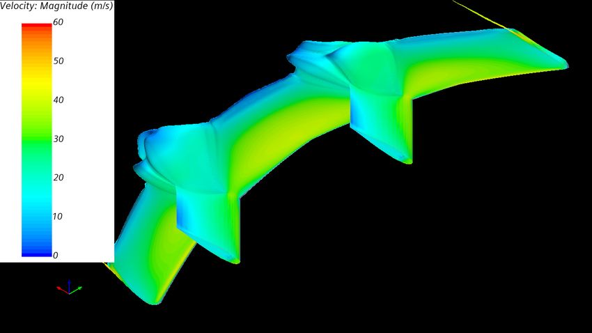
5 Results & Discussion - Wing and Pylon              Study                                                                                                               30
5.1 Reynolds Study . . . . . . . . . . . . . . . .   . . . . .   .   .   .   .   .   .   .   .   .   .   .   .   .   .   .   .   .   .   .   .   .   .   .   .   .   .   30
5.2 Wing Results & Normalization . . . . . . .       . . . . .   .   .   .   .   .   .   .   .   .   .   .   .   .   .   .   .   .   .   .   .   .   .   .   .   .   .   30
5.3 Pylons at reference position . . . . . . . . .   . . . . .   .   .   .   .   .   .   .   .   .   .   .   .   .   .   .   .   .   .   .   .   .   .   .   .   .   .   31
5.3.1 24cm pylon length . . . . . . . . . . . . .    . . . . .   .   .   .   .   .   .   .   .   .   .   .   .   .   .   .   .   .   .   .   .   .   .   .   .   .   .   31
5.3.2 10cm pylon length . . . . . . . . . . . . .    . . . . .   .   .   .   .   .   .   .   .   .   .   .   .   .   .   .   .   .   .   .   .   .   .   .   .   .   .   32
5.3.3 15cm pylon length . . . . . . . . . . . . .    . . . . .   .   .   .   .   .   .   .   .   .   .   .   .   .   .   .   .   .   .   .   .   .   .   .   .   .   .   33
5.4 Pylons moved rearward . . . . . . . . . . .      . . . . .   .   .   .   .   .   .   .   .   .   .   .   .   .   .   .   .   .   .   .   .   .   .   .   .   .   .   34
5.5 Pylons moved ahead . . . . . . . . . . . . .     . . . . .   .   .   .   .   .   .   .   .   .   .   .   .   .   .   .   .   .   .   .   .   .   .   .   .   .   .   35
5.5.1 10cm pylon length - Lofted top . . . . . .     . . . . .   .   .   .   .   .   .   .   .   .   .   .   .   .   .   .   .   .   .   .   .   .   .   .   .   .   .   35
5.5.2 15cm pylon length - Lofted top . . . . . .     . . . . .   .   .   .   .   .   .   .   .   .   .   .   .   .   .   .   .   .   .   .   .   .   .   .   .   .   .   36
5.5.3 15cm pylon length - Sliced top . . . . . .     . . . . .   .   .   .   .   .   .   .   .   .   .   .   .   .   .   .   .   .   .   .   .   .   .   .   .   .   .   37
5.6 Comparison of best results . . . . . . . . . .   . . . . .   .   .   .   .   .   .   .   .   .   .   .   .   .   .   .   .   .   .   .   .   .   .   .   .   .   .   39
5.7 Dependency on simulation conditions . . . .      . . . . .   .   .   .   .   .   .   .   .   .   .   .   .   .   .   .   .   .   .   .   .   .   .   .   .   .   .   41
5.8 Importance of Passive & Active Systems . .       . . . . .   .   .   .   .   .   .   .   .   .   .   .   .   .   .   .   .   .   .   .   .   .   .   .   .   .   .   42

6 Conclusion                                                                                                                                                             44

7 Future Work                                                                                                                                                            45

References                                                                                                                                                               46

                                                         vi
List of Figures
1.1 Schematic showing relative air yaw while cornering . . . . . . . . . . . . . . . . . . . . . . . . . 1
1.2 Focus areas for 3D and 2D studies . . . . . . . . . . . . . . . . . . . . . . . . . . . . . . . . . . 2
1.3 Global and local coordinate systems annotated on NACA0010 . . . . . . . . . . . . . . . . . . . 3
2.1 Domain size . . . . . . . . . . . . . . . . . . . . . . . . . . . . . . . . . . . . . . . . . . . . . . . 5
2.2 Coordinate system used for 2D studies . . . . . . . . . . . . . . . . . . . . . . . . . . . . . . . . 6
2.3 Prism layers near the airfoil . . . . . . . . . . . . . . . . . . . . . . . . . . . . . . . . . . . . . . 6
2.4 Refinement regions around the airfoil . . . . . . . . . . . . . . . . . . . . . . . . . . . . . . . . . 7
2.5 Mesh independence study performed on NACA0010 airfoil . . . . . . . . . . . . . . . . . . . . . 7
2.6 Example of an airfoil with passive and active systems . . . . . . . . . . . . . . . . . . . . . . . 9
3.1 Airfoils generated by optimizer using IGP . . . . . . . . . . . . . . . . . . . . . . . . . . . . . . 10
3.2 Julia optimisation history . . . . . . . . . . . . . . . . . . . . . . . . . . . . . . . . . . . . . . . 10
3.3 Airfoils selected for the study . . . . . . . . . . . . . . . . . . . . . . . . . . . . . . . . . . . . . 11
3.4 NACA0010 yaw sweep results . . . . . . . . . . . . . . . . . . . . . . . . . . . . . . . . . . . . . 12
3.5 NACA0010 yaw sweep velocity distribution . . . . . . . . . . . . . . . . . . . . . . . . . . . . . 12
3.6 Velocity scalar scene for NACA0010 with a 3mm wide notch placed at 5% chord length . . . . 13
3.7 Lift coefficients for NACA0010 with active suction . . . . . . . . . . . . . . . . . . . . . . . . . 13
3.8 Case 1 yaw sweep results . . . . . . . . . . . . . . . . . . . . . . . . . . . . . . . . . . . . . . . . 14
3.9 Case 1 yaw sweep velocity distribution . . . . . . . . . . . . . . . . . . . . . . . . . . . . . . . 14
3.10 Case 1 yaw sweep results with passive system . . . . . . . . . . . . . . . . . . . . . . . . . . . . 15
3.11 Case 1 yaw sweep velocity distribution with passive system . . . . . . . . . . . . . . . . . . . . 15
3.12 Case 1 yaw sweep results with active system . . . . . . . . . . . . . . . . . . . . . . . . . . . . . 16
3.13 Case 1 yaw sweep velocity distribution with active system . . . . . . . . . . . . . . . . . . . . . 16
3.14 Case 2 yaw sweep results before tweaking . . . . . . . . . . . . . . . . . . . . . . . . . . . . . . 17
3.15 Case 2 yaw sweep velocity distribution before tweaking . . . . . . . . . . . . . . . . . . . . . . . 17
3.16 Case 2 yaw sweep results after tweaking . . . . . . . . . . . . . . . . . . . . . . . . . . . . . . . 17
3.17 Case 2 yaw sweep velocity distribution after tweaking . . . . . . . . . . . . . . . . . . . . . . . 18
3.18 Case 2 yaw sweep results with passive system . . . . . . . . . . . . . . . . . . . . . . . . . . . . 18
3.19 Case 2 yaw sweep velocity distribution with passive system . . . . . . . . . . . . . . . . . . . . 19
3.20 Case 2 yaw sweep results with active system . . . . . . . . . . . . . . . . . . . . . . . . . . . . . 19
3.21 Case 2 yaw sweep velocity distribution with active system . . . . . . . . . . . . . . . . . . . . . 19
3.22 Case 3 yaw sweep results . . . . . . . . . . . . . . . . . . . . . . . . . . . . . . . . . . . . . . . . 20
3.23 Case 3 yaw sweep velocity distribution . . . . . . . . . . . . . . . . . . . . . . . . . . . . . . . 20
3.24 Case 3 yaw sweep results with passive system . . . . . . . . . . . . . . . . . . . . . . . . . . . . 21
3.25 Case 3 yaw sweep velocity distribution with passive system . . . . . . . . . . . . . . . . . . . . 21
3.26 Case 3 yaw sweep results with active system . . . . . . . . . . . . . . . . . . . . . . . . . . . . . 22
3.27 Case 3 yaw sweep velocity distribution with active system . . . . . . . . . . . . . . . . . . . . . 22
3.28 Comparison of the force coefficients for the generated optimized airfoils . . . . . . . . . . . . . 23
3.29 Drag comparison of the generated passive designs . . . . . . . . . . . . . . . . . . . . . . . . . . 23
3.30 Lift comparison of the generated passive designs . . . . . . . . . . . . . . . . . . . . . . . . . . 24
3.31 Comparison of the force coefficients for the generated active designs . . . . . . . . . . . . . . . 24
4.1 Wing + Pylon Isometric view . . . . . . . . . . . . . . . . . . . . . . . . . . . . . . . . . . . . . 25
4.2 Computational Domain & Boundaries . . . . . . . . . . . . . . . . . . . . . . . . . . . . . . . . 26
4.3 Volume mesh around the wing at Y = 0, seen from left (-Y-direction) . . . . . . . . . . . . . . 27
4.4 Force coefficients vs number of mesh cells . . . . . . . . . . . . . . . . . . . . . . . . . . . . . . 27
4.5 Position of the left pylon (24cm length) along with reference point, from -X axis . . . . . . . . 28
4.6 24cm pylons at reference position . . . . . . . . . . . . . . . . . . . . . . . . . . . . . . . . . . . 28
4.7 10cm pylons moved rear . . . . . . . . . . . . . . . . . . . . . . . . . . . . . . . . . . . . . . . . 28
4.8 15cm pylons moved ahead . . . . . . . . . . . . . . . . . . . . . . . . . . . . . . . . . . . . . . . 28
5.1 Reynolds study of CL for positive yaw angle sweep . . . . . . . . . . . . . . . . . . . . . . . . . 30
5.2 Velocity magnitude over isosurface of CP = 0 for 24cm pylons at 0◦ yaw . . . . . . . . . . . . . 31
5.3 Velocity magnitude over isosurface of CP = 0 for 24cm pylons at +15◦ yaw . . . . . . . . . . . 31
5.4 Velocity magnitude over isosurface of CP = 0 for 10cm pylons at 0◦ yaw . . . . . . . . . . . . . 32
5.5 Velocity magnitude over isosurface of CP = 0 for 10cm pylons at +15◦ yaw . . . . . . . . . . . 33
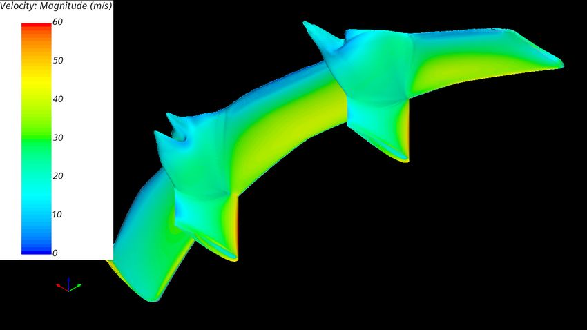
5.6 Velocity magnitude over isosurface of CP = 0 for 15cm pylons at +15◦ yaw . . . . . . . . . . . 34
vii5.7 Velocity magnitude over isosurface of CP = 0 for 10cm pylons moved rear at +15◦ yaw . . . . . 35
5.8 Velocity magnitude over isosurface of CP = 0 for 10cm pylons moved ahead at 0◦ yaw . . . . . 35
5.9 Velocity magnitude over isosurface of CP = 0 for 10cm pylons moved ahead at +15◦ yaw . . . 36
5.10 Velocity magnitude over isosurface of CP = 0 for 15cm pylons moved ahead at 0◦ yaw . . . . . 36
5.11 Velocity magnitude over isosurface of CP = 0 for 15cm pylons moved ahead at +15◦ yaw . . . 37
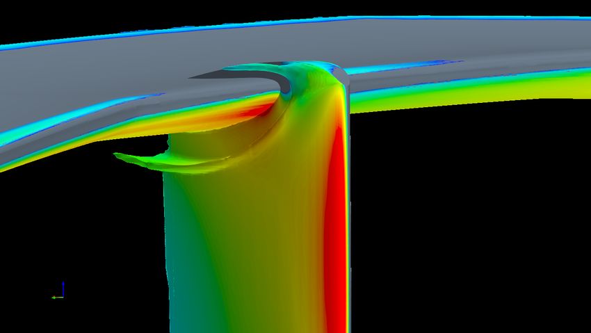
5.12 Case 2 right pylon with lofted top at +15◦ yaw . . . . . . . . . . . . . . . . . . . . . . . . . . . 38
5.13 Case 2 right pylon with sliced top at +15◦ yaw . . . . . . . . . . . . . . . . . . . . . . . . . . . 38
5.14 Velocity magnitude over isosurface of CP = 0 for 15cm pylon with sliced top at +15◦ yaw . . . 38
5.15 Velocity magnitude over isosurface of CP = 0 for 15cm pylons with sliced top at 0◦ yaw . . . . 39
5.16 Normalized spanwise lift distribution over the wing for +15◦ yaw angle . . . . . . . . . . . . . . 40
5.17 Force coefficients for a sweep study of best wing and pylon combinations . . . . . . . . . . . . . 41
5.18 Normalized spanwise lift distribution over the wing for +15◦ yaw angle . . . . . . . . . . . . . . 42
5.19 Averaged CL values for Case 2 at different Reynolds number . . . . . . . . . . . . . . . . . . . 43
5.20 Force coefficients for a sweep study of moved ahead Case 2 pylon with lofted top . . . . . . . . 43
viiiList of Tables
2.1 Ranges for parameters defining the airfoil . . . . . . . . . . . . . . . . . . . . . . . . . . . . . . 8
3.1 Parameters defining the airfoil . . . . . . . . . . . . . . . . . . . . . . . . . . . . . . . . . . . . . 11
4.1 Pylon position & length combinations for simulation . . . . . . . . . . . . . . . . . . . . . . . . 29
5.1 Results for the wing . . . . . . . . . . . . . . . . . . . . . . . . . . . . . . . . . . . . . . . . . . 31
5.2 Results for 24cm pylon at reference position . . . . . . . . . . . . . . . . . . . . . . . . . . . . . 32
5.3 Results for 10cm pylon at reference position . . . . . . . . . . . . . . . . . . . . . . . . . . . . . 32
5.4 Results for 15cm pylon at reference position . . . . . . . . . . . . . . . . . . . . . . . . . . . . . 33
5.5 Results for 10cm pylon moved rear, at +15◦ yaw . . . . . . . . . . . . . . . . . . . . . . . . . . 35
5.6 Results for 10cm pylon after moving ahead . . . . . . . . . . . . . . . . . . . . . . . . . . . . . 36
5.7 Results for 15cm pylon after moving ahead . . . . . . . . . . . . . . . . . . . . . . . . . . . . . 37
5.8 Results for 15cm pylons moved ahead with sliced top . . . . . . . . . . . . . . . . . . . . . . . . 39
5.9 Best results for wing and pylon study . . . . . . . . . . . . . . . . . . . . . . . . . . . . . . . . 39
ixx
1 Introduction
The margin between the lap timings of performance cars is getting narrower by the day. To battle these narrow
margins, care must be given to the smallest of the parts which may be overlooked at times. One such area can
be the pylon section of a rear wing that connects to the car. A thorough study on the implementation of active
flow controls and passive slotted designs to the pylons could bring out potential performance improvements, in
this case, cornering performance.
Automobili Lamborghini S.p.A is one of the foremost super sports cars manufacturers in the world, and
since their innovative system of active aerodynamics, Aerodinamica Lamborghini Attiva (ALA)[2] took hold,
the concept of super sports cars performance has been taken to levels not seen before. The rear wings of the
cars with ALA system equipped, work on the principal of active flow control to improve performance of the
vehicle[3][4]. The rear wing on the cars is used to generate large amounts of downforce, helping the vehicle to
stay on track at higher speeds. The downforce generation is exceptionally important while executing turns.
Improving the downforce can enhance the car’s cornering speeds and therefore the lap timings. Although this
effect is beneficial for achieving faster lap times, it comes with a penalty of higher drag force. Designing the
car’s rear wing for a better cornering performance and downforce improvement with very little drag penalty
can be a bit challenging. In this thesis, pylons would be redesigned to compensate for changes in the yaw
angles, making the rear wing more robust against the higher yaw angles. A detached flow under the wing
hampers the performance significantly. This upgrade is expected to improve the performance in two ways.
First, improve flow around the suction side of the wing, creating more downforce. Second, generate forces in
the lateral direction to improve cornering stability. The scope for air yaw angle in this study ranges from −15◦
to +15◦ based on an investigation performed by Oskar Hellsten & Oskar Pettersson[5] for high performance car.
Figure 1.1: Schematic showing relative air yaw while cornering
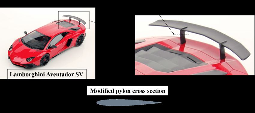
Figure 1.1 is annotated to explain how the study was carried out on the rear wing of Lamborghini Aventador
SV. When a car is cornering, in this case taking a right turn, the yaw moment about car center would pull the
front of the car into the corner but push the rear outwards. Due to this, the relative motion between the wing
and air is rotated that generated forces in +X and +Y directions. The coordinate system used throughout this
thesis was a local coordinate system that moves with the car. For this thesis, the convention maintained was
that the car taking a right turn resulted in a positive yaw angle flow, and the right pylon would be the one
downstream and placed over the inner wheels. Ensuring high downforce over the inner wheels is of utmost
importance during cornering. Figure 1.2 provides a greater insight into the area of focus. It has a representative
1cross-section of the pylon and not the actual cross-section of the pylons. Lamborghini Aventador SV has a dual
pylon wing assembly, making it symmetric. Thus, an asymmetric airfoil which required a study performed in
positive and negative yaw angles, when converted to a 3D pylon along with the wing was simulated for only
positive yaw angles. Cross-section of the pylon was optimized during the 2D study to ensure attached flow
around the pylons. While, only the wing and pylon assemblies were considered in 3D study.
Figure 1.2: Focus areas for 3D and 2D studies
1.1 Purpose
The objective of this master thesis was to propose new pylon designs for the wing and to perform aerodynamic
studies introducing passive and active flow control measures for performance optimization. As no optimization
work was carried out on the wing in this thesis, the goal of the proposed pylon designs was to match or improve
the downforce generated by the wing without pylons, while mitigating drag penalties at lower yaw angles.
The scope for the pylon studies ranges from yaw angles between +15◦ to -15◦ . This thesis also addressed the
following questions;
• Can asymmetric airfoils produce better averaged lift forces than symmetric airfoils in the local coordinate
system?
• How does the geometry and positioning of the passive or active system affect performance of the airfoil?
• What are the pros and cons of passive and active systems?
• Why was a single slot passive system implemented over dual slot?
• Can a single slot passive system perform well in positive as well as negative yaw conditions?
• How does the size, placement and the geometry of the pylon affect the performance of the rear wing?
• Do the results from the 2D airfoil study correlate to the results obtained from 3D wing and pylon study?
• Is it necessary to use active and passive systems to maintain attached flow within the yaw angle scope?
1.2 Literature Study
This thesis is a successor to another master thesis performed in 2020 by Oskar Hellsten & Oskar Pettersson,
titled ’A novel approach to the design of rear airfoil pylons on high performance car’[5]. The focus of the
previous thesis was on symmetric airfoils and the implementation of passive systems for flow improvement,
2which provided a good foundation to build upon. Based on their work, NACA0010 was chosen as the reference
airfoil for this thesis. Even after optimising symmetric airfoils for low drag performance, NACA0010 was
undefeated at lower yaw angles. However, the trade-off for this airfoil was the stalling at high yaw angles.
For the airfoil study in this thesis, a low Reynolds number (≈ 695000) was chosen. A study performed on
NACA0009 and NACA0012 to understand the airfoil characteristics at low Reynolds number[6] provided deeper
insights into the performance expectations of NACA0010. The simulations backed by experimental correlation
helped shape the approach for designing optimum airfoils for this thesis.
Theory of Wing Sections[7] provided the initial overview of this topic. The plethora of airfoil data doc-
umented in this book along with the literature on passive systems were crucial for our airfoil designs. Another
interesting concept for improving flow using a passive system was achieved by introducing a small notch over
NACA4412[8]. However, this concept reduced the separations but unable to maintain attached flow at higher
angles of attack. The book Competition Car Aerodynamics[9] was extremely helpful and gave a general idea
about wing designs and parameters. It also helped to define the range of airfoil design parameters for optimizing
asymmetric airfoils. Most of the asymmetric airfoils researched online produced good lift in one direction,
but stalled early in the other direction. As our use case was dependant on maximum average lift, most of
the research on asymmetric airfoils did not meet our criterion. Some of the common airfoils like NACA0012,
NACA2412, NACA4415 and NACA63-215 performed similar to NACA0010 at lower yaw angles when the
values were averaged for positive and negative angles of attack. This comparison was made possible through
the vast data available on Airfoil Tools[10]. In this thesis, we used the two coordinate systems to our advantage
by allowing the asymmetric airfoils to have global rotation as well. Thus, the airfoil chords need not align with
the X direction.
The airfoil studies are generally performed using a global coordinate system, where the airfoil is rotated
by said angle of attack and the flow direction is kept constant along with the coordinate system. Thus, the
airfoil would not lie along the coordinate system at an angle greater than 0◦ . However, in this thesis, a local
coordinate system was implemented by keeping the airfoil fixed, while the air flow was rotated to simulate the
yaw angle. The Figure 1.3 shows the differences between the two systems when an angle of attack exists. The
+X and +Y axes are fixed and denote drag and lift forces respectively. When the first approach is used, both
the drag and lift forces increase when the angle of attack is increased, until the airfoil stalls. This was noticed
through the airfoil data presented in the book Theory of Wing Sections mentioned above and also through
Airfoil Tools[10]. However, when the local coordinate system was used, the drag forces started to decrease as
the yaw angle increased. While, the lift continued to increase. Again, this held true until the wing stalled.
After stalling, the lift forces reduced while the drag force increased.
Figure 1.3: Global and local coordinate systems annotated on NACA0010
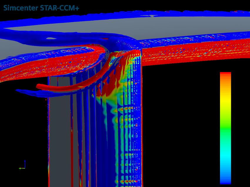
The geometry and simulation pictures presented in this report were taken from STAR-CCM+[11], while all the
plots reported were generated using MATLAB[12].
31.3 Limitations
As the thesis is spanned for 20 weeks, the duration of the project is a major limitation. The quest to find
an optimum pylon design is a long process and is time bounded. The following points may be considered as
limitations for this thesis;
• 3D simulations on the wing and pylon combinations were carried out without a car body, and were
suspended mid air.
• By using Reynolds Averaged Navier Stokes solver, we were unable to see the effect of active and passive
systems in real time. On a race track, the yaw angles vary rapidly, and it is important that the passive
and active systems can operate efficiently to meet such demands.
• Active flow control implemented had a fixed flow rate, and could not be increased to significantly improve
the robustness against high angle of attack.
• Manufacturing capabilities were considered while designing the airfoil, especially for fillets. This proved
to hinder the performance when compared to a completely conceptual airfoil design.
• The pylons were optimized aerodynamically and did not undergo any structural tests. However, the
designs are not impractical as they have been discussed and agreed upon by experienced supervisors.
42 Airfoil Study
This chapter explains the pylon airfoil geometry considerations, computational domain size, boundary conditions
and other details related to the CFD pre-processes for a two-dimensional study of airfoils. Furthermore, details
regarding the passive and active flow controls will be described. This section focuses on the study related to
the pylon’s airfoil geometry in 2D. This 2D study stands as a base for the 3D pylons used in Section 4.
2.1 Simulation Overview
To carry out any CFD simulations it is essential to define a flow region or the domain size. The size of the
domain must be chosen in such a way that it captures all the necessary flow interaction without being very
large. A larger domain size comes with a consequence of longer simulation run times and higher computational
costs. After careful considerations, a computational domain of 8m width (≈ 30 times the chord length) and
14m length (≈ 50 times the chord length) was implemented as seen in Figure 2.1. The model was placed at a
distance of 4m along the X-axis from the flow inlet boundary, and midway of the 8m width (Y-axis).
Figure 2.1: Domain size
2.1.1 Coordinate System & Force Coefficients
The coordinate system used for the 2D studies is shown in Figure 2.2. Positive X-direction is towards the outlet
of the domain and positive Y-direction is towards the top of the domain. The drag of the airfoil is considered
to be in the positive X-direction and the lift is measured in the Y-direction. The positive and negative lift
follows the same sign convention as the Y-axis (positive Y-axis has a positive lift and vice-versa). Lift of the
airfoil becomes the side force of the car and the drag remains the same. The equations for the non-dimensional
force coefficients are mentioned below.
2 ∗ Fx 2 ∗ Fy
CD = (2.1) CL = (2.2)
ρ ∗ v2 ∗ A ρ ∗ v2 ∗ A
Here, CD is the coefficient of drag and CL the coefficient of lift while, ρ denotes the density of air at
25°C i.e. 1.184 kg/m3 , v denotes velocity (38.8 m/s), A denotes the chord length of the airfoil for a 2D study.
As the airfoil lengths vary marginally, the Reynolds number for this study is equivalent to ≈ 695, 000.
5Figure 2.2: Coordinate system used for 2D studies
2.1.2 Solver and flow parameters
The simulations were performed using Reynolds-Averaged Navier Stokes (RANS) solver. SST K-Omega
Turbulence model developed by F. Menter[13] was used in this study. Incompressible flow was assumed since
the flow velocity does not exceed Mach 0.3. Flow velocity of the air was set to 140Km/h or 38.89m/s as
asked by Automobili Lamborghini S.p.A. For the positive yaw sweeps, the flow inlet and the bottom of the
domain were set as the velocity inlets, while the top of the domain and flow outlet of the domain were set as
the pressure outlets. For negative yaw sweeps, the flow inlet and the top of the domain were set as the velocity
inlet, the bottom of the domain and the flow outlet of the domain were set as the pressure outlet.
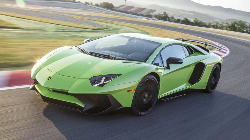
2.2 Mesh Study
Mesh study is a process of checking the dependency of the solutions based on the refinement in mesh cell
size. This study aims to find a mesh with sufficiently high accuracy while keeping the computational cost low.
In the earlier phase of the thesis, it was decided to keep the airfoil’s position in the domain fixed and vary
the direction of the fluid (in this case air) to achieve the yaw changes. This helps in avoiding re-meshing by
keeping the same mesh constraints for all yaw angles. Polyhedral mesher was used. To capture the viscous
boundary layer, All Y+ Wall Treatment was used and Y+ values were maintained between 1 to 5. To achieve
this, the number of prism layers were set to 13 and the thickness of the prism layers to be 2mm, this can be
seen in Figure 2.3. To capture a better flow resolution, multiple refinement regions were introduced; near-airfoil
offset region, trailing edge refinement, near-wake refinement region and farther wake refinement region. These
refinement regions can be observed in Figure 2.4.
Figure 2.3: Prism layers near the airfoil
6Figure 2.4: Refinement regions around the airfoil
A mesh independence study was carried out on the NACA0010 airfoil to ensure that the results were not
influenced by the current mesh settings. Figure 2.5 shows the drag coefficient for 0◦ yaw and lift coefficient
for 12.5◦ yaw, for varying meshes. As 15◦ yaw angle resulted in completely detached flow, it was better to
perform lift analysis on 12.5◦ yaw angle instead. The smallest cell size tested was 1.75mm. It was observed
that increasing the number of cells beyond 3mm base size did not result in significant changes for either case.
Thus, 3mm base size (≈ 80k cells) was used for all the simulations in 2D study. The surface cells on the airfoil
were half of the base size.
(a) Coefficient of drag at 0◦ yaw (b) Coefficient of lift at 12.5◦ yaw
Figure 2.5: Mesh independence study performed on NACA0010 airfoil
2.3 Airfoil Optimization
In the earliest stage of the thesis, it was concluded to set the NACA0010 airfoil as the baseline for the
development of other airfoil profiles. This decision was based on the low drag performance at lower yaw
angles, as studied in a previous thesis[5]. The NACA0010 profile was obtained from Airfoil Tools (2021)[10]. A
7surrogate-based optimizer tool created by Magnus Urquhart[14] using the programming language Julia[15] was
utilized to optimize the airfoil profiles. The optimizer works on the principle of minimizing the target value. As
this study was for a dual pylon approach, the average of absolute lift values generated at +7.5◦ and −7.5◦ were
maximized (negative lift values were minimized). This condition was selected so that a balance between low
drag and high lift can be achieved at 0◦ and 15◦ yaw angles respectively.
The optimization was performed by running a Julia script that had an embedded MATLAB code to generate
airfoils based on various parameters. This code utilized the IGP[16] function that uses nine variables to generate
data points for the corresponding airfoil. Out of the nine parameters, eight were airfoil design parameters
while the remaining one defined the resolution of data points which was set to 300. These airfoils were given
an additional parameter, rotation concerning the global coordinates. Thus, a total of nine parameters were
defining the range of optimization and this can be seen in Table 2.1.
Parameter Range
Global Rotation -2.5 to +2.5
c1 0 to 2
Camber line abscissa coefficient
c2 0 to 2
c3 0 to 1
Camber line ordinate coefficient
c4 0 to 0.3
Maximum thickness 0.05 to 0.3
Maximum thickness position 0.1 to 0.3
Relative leading edge radius 0.2 to 4
Relative trailing edge radius 0.5 to 4
Table 2.1: Ranges for parameters defining the airfoil
2.4 Passive and Active Systems
The thesis aims to improve the performance of the airfoils at yaw angles of up to 15◦ both in +ve and -ve yaw
conditions. Tests were conducted to study the performance of the generated airfoils for an array of yaw angles
up to 15◦ . To tackle separation occurring at higher yaw angles, passive and active systems were implemented
on the airfoil to attach the flow.
2.4.1 Passive system
The passive system is implemented using the slotted design of airfoils as seen in Figure 2.6a. The slot guides
the air from one side in order to attach the flow on the other side. However, this approach comes with the
penalty of disturbing the flow in other direction. Thus, the optimized airfoils were vital in considering this
approach. The optimum slot for a profile was decided by the highest average lift values at ±15◦ yaw angle. A
dual (cross) slot system was previously explored in the thesis[5] that preceded this. Dual slot was incapable of
providing attached flow in either direction at higher yaw angles. The single slot approach aimed at improving
the flow on one side of the pylon, and would be focused at improving performance over the inner wheel while
cornering. Thus, a single slot approach better suited the purpose of this thesis.
2.4.2 Active system
The active system implemented was basically a flow control method, either by blowing the flow tangential to
the airfoil surface using a slot, or by creating a suction normal into the airfoil using a notch. These methods
solve the problem of detached flow at higher yaw angles. For the blowing method, a stagnation inlet was used
to mimic the ALA system[2]. Using a 3mm slot, the stagnation inlet was set at 533P a based on a fraction of
the flow speed. This condition was fixed for the blowing method as any slot below 3mm would be difficult
to manufacture, while a larger slot would disturb the flow further, especially when it is inactive. Also, an
increased slot would have a reduced flow speed as a similar flow rate was to be maintained. This active slot
was tested across various positions along the chord length for each profile to ensure optimum performance.
An example of the active blowing approach is shown in Figure 2.6b, where the wind annotation signifies the
blowing slot in +X direction.
8The idea behind alternative active approach, motorized suction, was to expend energy in order to create a
suction that maintained a constant flow rate. This was implemented using a negative velocity inlet on the
notch created over the airfoil surface (shown in Figure 3.6). With efficiency in question, this method was
only implemented when the blowing method was ineffective. For suction, the velocity could be varied as it
is controlled, but it was important to consider power consumption for the ideal design. This method also
results in complex construction and manufacturing of parts. These limitations can offset the purpose of the
active systems to improve the car’s aerodynamic performance. However, with a notch design, the airfoil would
not undergo a significant redesign, unlike a slot for active blowing. Thus, it can be placed before the point
maximum thickness, which makes it effective on designs that have detached flow right at the leading edge.
(a) Passive (b) Active
Figure 2.6: Example of an airfoil with passive and active systems
93 Results & Discussion - Airfoil Study
In this section, the generated airfoils and results of the airfoil performance will be presented in steps starting
from NACA0010 which was considered as the base profile. Other generated airfoil profiles will follow after
presenting the base profile. The sweep study is performed in intervals of 1◦ between 0◦ and 5◦ , while the
interval increases to 2.5◦ between 5◦ and 15◦ yaw angles.
3.1 Generated Airfoils
The range of parameters defined in Table 2.1 were used by the surrogate model to test out various airfoils.
With freedom to generate asymmetric airfoils, the surrogate model varied the parameters in order to arrive at
profiles with best lift capabilities at ±7.5◦ yaw. Figure 3.1 shows a cluster of airfoils generated by the optimizer.
The generated airfoils were simulated in STAR-CCM+ for both the angles.
Figure 3.1: Airfoils generated by optimizer using IGP
Figure 3.2: Julia optimisation history
Figure 3.2 shows an example of how the optimizer iterated to achieve maximum lift. The Y axis denotes the
summation of negative lift values at ±7.5◦ yaw. The orange dots resemble the lift values at a specific iteration.
10The optimizer ran for many such loops which generated numerous profiles and were tested in STAR-CCM+
until the lift values saw insignificant improvements and the parameters defining the airfoils started to saturate.
As the parameter range was wide, some of the generated airfoils performed badly. These outliers can be
evidently seen in Figures 3.1 and 3.2. Some airfoils generated were self intersecting as well and could not be
simulated in STAR-CCM+.
After running the optimizer a couple of times, three airfoils were selected based on their performances.
The parameters defining these airfoils can be seen in Table 3.1. Both abscissa coefficients were capped at 1 for
Case 1. All three cases have different thicknesses and were arranged in an increasing order. Between Case
2 and Case 3, all parameters except maximum thickness were quite similar. All parameters other than the
trailing edge radius were well within the defined ranges. Thus, they are not bounded by the range. It was
interesting to see how the optimizer focused on making the trailing edge thinner. Manufacturing constraints
needed to be considered, thus 0.5 was set as the minimum limit.
Airfoils
Parameters
Case 1 Case 2 Case 2
Global Rotation -0.38 -0.58 -0.36
c1 1.00 1.69 1.73
Camber line abscissa coefficient
c2 1.00 1.09 1.09
c3 0 0 0
Camber line ordinate coefficient
c4 0.02 0.04 0.04
Maximum thickness 0.11 0.13 0.15
Maximum thickness position 0.23 0.26 0.26
Relative leading edge radius 0.50 0.59 0.57
Relative trailing edge radius 0.79 0.50 0.50
Table 3.1: Parameters defining the airfoil
Figure 3.3: Airfoils selected for the study
Figure 3.3 represents the three best designs which were selected from the generated lot of profiles. The selection
11was based on the airfoil performances at low and high yaw angles. It can be observed that thicknesses of the
selected airfoils are larger than the NACA0010 profile, as it helps accelerate flow around the leading edge at
greater yaw angles. The global rotation was not included in the airfoil plots. This was implemented when the
airfoils were imported in STAR-CCM+, where it was also ensured that none of the airfoils had a trailing edge
thickness lesser than 1mm.
3.2 NACA0010
Yaw sweep was performed on the NACA0010 airfoil at 140Km/h and the following results were obtained. Since
the airfoil is symmetric, only positive yaw results are shown. The sweep study shows that the NACA0010
airfoil keeps the flow attached till 12.5◦ yaw and detaches at 15◦ yaw. This can be seen from Figure 3.5. Being
a thin airfoil, NACA0010 had the lowest drag amongst other airfoils studied in the previous thesis[5]. However,
that results in a lower robustness against high yaw angles.
(a) Coefficient of drag (b) Coefficient of lift
Figure 3.4: NACA0010 yaw sweep results
(a) 12.5◦ yaw (b) 15◦ yaw
Figure 3.5: NACA0010 yaw sweep velocity distribution
Implementing a passive system is not suitable for NACA0010 as it has a completely detached flow for ±15◦ .
Attached flow on one side could be observed by adding a slot, however, the opposite flow was ruined for middle
yaw angles too. Passive system for NACA0010 was not included in this study as it was not an optimal result.
123.2.1 NACA0010: Active
Earlier the separation occurs, the greater is the demand from the active system to pull in the entire airflow.
With a stagnation inlet approach, a high velocity could not be achieved, thus the blowing approach could not
be placed closer to the leading edge as that region needs to have high accelerated flow for attachment. Hence,
the active system was placed further back along the chord length. After testing out all positions along the
chord length, this approach was discarded. The other active method in our project scope was to provide a
motorized suction. To simulate this system, a constant negative velocity inlet was introduced over the body of
the airfoil as seen in Figure 3.6. With this approach, attached flow could be achieved for +15◦ yaw, while the
−15◦ case would still have detached flow.
(a) Flow with suction active at +15◦ yaw (b) Close up on the notch at +15◦ yaw
Figure 3.6: Velocity scalar scene for NACA0010 with a 3mm wide notch placed at 5% chord length
With a maximum suction of 30m/s available, a sensitivity analysis was conducted to find the optimum position
and suction velocity as seen in Figure 3.7a. Even though the maximum speed was defined, 35m/s was tested to
see the saturating trend of results. Speeds below 30m/s at 10% chord length were struggling to keep the flow
attached, and did not work at all below 20m/s. From this study, it was concluded that a suction at 7.5% chord
length with speed on 25m/s is optimum. A sweep study was performed on all these combinations, and as seen
in Figure 3.7b, the boost in performance is immense beyond +12.5◦ yaw.
(a) Sensitivity to position and suction speed at +15◦ yaw (b) Positive sweep study on the various active configurations
Figure 3.7: Lift coefficients for NACA0010 with active suction
133.3 Case 1
The earlier NACA0010 airfoil was a symmetric profile. The Case 1 airfoil is an asymmetric profile along with
−0.4◦ rotation. The airfoil generated also has a maximum thickness greater than the NACA0010 profile. The
flow attachment at higher yaw condition can be observed from Figure 3.9b. However, the +15◦ yaw still has
flow detachment. This can be improved by the passive and active systems as mentioned earlier. As the negative
yaw rotation of the airfoil helps the flow to stay attached for a bit longer in the negative yaw side of the
airfoil, passive system can be used to aid the positive air flow. It is to be noted that the graphs contain both
yaw conditions in the same axes. The negative yaw results, in actuality have the opposite sign to that of the
positive yaw results. To make the comparison easier, both conditions were represented in the same graph by
keeping the same sign convention. Overall, when the positive and negative yaw lift values were averaged, Case
1 outperformed the NACA0010 with a drag penalty of 1 count.
(a) Coefficient of drag (b) Coefficient of lift
Figure 3.8: Case 1 yaw sweep results
(a) +15◦ yaw (b) -15◦ yaw
Figure 3.9: Case 1 yaw sweep velocity distribution
3.3.1 Case 1: Passive
The slot of the passive design was placed at 38% of the chord length, this can be observed in Figure 3.11. The
results for the passive system are presented in Figure 3.10. From the graph in Figure 3.10b it can be seen
that the passive system at +15◦ yaw generates a lift of 1.437. In the negative yaw the system generates a lift
14of 1.107. The base profile however, has better performance in terms of lift and drag until 12.5◦ yaw. This is
because the passive designs were optimized for +15◦ yaw conditions. The negative yaw angle performance
for this design was not bad, especially at lower yaw angles. The negative separation gradually increases with
increasing yaw angle.
(a) Coefficient of drag (b) Coefficient of lift
Figure 3.10: Case 1 yaw sweep results with passive system
The averaged lift values for the 15◦ yaw condition for this passive design provides a 1.272 lift. This is better when
compared with the base Case 1 airfoil’s average lift of 1.213. This highlights the con of passive system. While
it increases performance at the yaw angle where a closed profile would have a detached flow, its performance is
sub-par at angles below detachment angle.
(a) +15◦ yaw (b) -15◦ yaw
Figure 3.11: Case 1 yaw sweep velocity distribution with passive system
3.3.2 Case 1: Active
The graphs shown in Figure 3.12 represent the positive yaw results of the active system. The active slot for
blowing was placed at 24% chord length position. Since there are no geometry changes in the negative side,
the results remained similar to the base Case 1 airfoil’s negative yaw performance. The scalar scene shown in
Figure 3.13b has a very good flow attachment. It can be seen that the inactive condition performs very similar
to the Case 1’s base airfoil’s performance at angles below +15◦ yaw. At +15◦ yaw, the active blowing can be
started to improve the performance drastically. Thereby, proving the effectiveness of the active system in this
case.
15(a) Coefficient of drag (b) Coefficient of lift
Figure 3.12: Case 1 yaw sweep results with active system
(a) +15◦ yaw (b) Zoomed in scalar scene
Figure 3.13: Case 1 yaw sweep velocity distribution with active system
3.4 Case 2
Case 2 airfoil is an asymmetric airfoil similar to Case 1 but the differences lie in the rotation and thickness
of the profile. Case 2 is slightly thicker and has −0.58◦ rotation. As seen from Figure 3.14, Case 2 performs
better than NACA0010 at higher yaw angles, while facing a drag increment of 2 counts at 0◦ yaw angle. Unlike
Case 1, Case 2 results in decent flow attachment even at ±15◦ yaw angle.
After an iterative process, the Case 2 design was rotated by −1◦ instead of −0.58◦ . With this change, the CL
at −15◦ yaw angle increased by 5 counts, however the +15◦ yaw angle CL reduced by 29 counts. This was done
in order to improve the utilisation of passive and active systems as they would be implemented to improve
positive yaw flow. The updated results can be seen in Figure 3.16. It was observed that the average value at 15◦
yaw has dropped with this tweak, and there was a greater disparity between the positive and negative sweep
results. The tweaked configuration (−1◦ rotation) was used for passive and active system implementation.
16(a) Coefficient of drag (b) Coefficient of lift
Figure 3.14: Case 2 yaw sweep results before tweaking
(a) +15◦ yaw (b) -15◦ yaw
Figure 3.15: Case 2 yaw sweep velocity distribution before tweaking
(a) Coefficient of drag (b) Coefficient of lift
Figure 3.16: Case 2 yaw sweep results after tweaking
17(a) +15◦ yaw (b) -15◦ yaw
Figure 3.17: Case 2 yaw sweep velocity distribution after tweaking
3.4.1 Case 2: Passive
The slot for this case was placed at 45% chord length and can be observed in Figure 3.19. When compared
with the Case 1’s placement of the slot, the slot is pushed further towards the trailing edge of the airfoil. This
is due to comparatively delayed detachment of the flow at 15◦ yaw conditions. Figure 3.18b shows the lift
performance of the Case 2 passive design. A maximum lift value of 1.501 can be observed in the +15◦ yaw,
which is much higher than the Case 1’s passive system average. However, in −15◦ yaw, the passive design only
provides a lift value of 1.013, this is comparatively lower to Case 1’s negative yaw passive system performance.
This design fetches a good average performance over the positive and negative yaw sweeps, with a maximum
averaged lift value of 1.264. The average lift values of this are better by 17 drag counts when compared to the
tweaked (base) Case 2 airfoil’s average.
3.4.2 Case 2: Active
The outlet for Case 2’s active slot was placed at around 45% chord length similar to the passive system. The
positive yaw performance has excellent flow attachment at +15◦ yaw which can be noticed in Figure 3.21. The
difference between the base Case 2 and the inactive performance of this airfoil is very small which can be
observed in Figure 3.20b. Thus, once again, the active system can work efficiently by activating only above
+10◦ yaw angle. With good results in negative yaw sweep (same as the base case), this is a very good outcome.
(a) Coefficient of drag (b) Coefficient of lift
Figure 3.18: Case 2 yaw sweep results with passive system
18(a) +15◦ yaw (b) -15◦ yaw
Figure 3.19: Case 2 yaw sweep velocity distribution with passive system
(a) Coefficient of drag (b) Coefficient of lift
Figure 3.20: Case 2 yaw sweep results with active system
(a) +15◦ (b) Zoomed in scalar scene
Figure 3.21: Case 2 yaw sweep velocity distribution with active system
193.5 Case 3
The Case 3 profile is the thickest of the airfoils selected and has a rotation of −0.36◦ . The trend for lift
coefficient of this case was quite similar to each other at positive and negative yaw conditions shown in Figure
3.22b. Case 3 average CL always performed better than NACA0010. However, at 0◦ yaw, Case 3 had 2 counts
greater drag. It can be seen that the flow detached a bit later than the Case 2 airfoil’s base profile. However,
the lift performance did not improve when compared to the Case 2. Their performances were quite similar
throughout the sweep as Case 2 performed slightly than Case 3 at 15◦ yaw.
(a) Coefficient of drag (b) Coefficient of lift
Figure 3.22: Case 3 yaw sweep results
(a) +15◦ yaw (b) -15◦ yaw
Figure 3.23: Case 3 yaw sweep velocity distribution
3.5.1 Case 3: Passive
When compared to the passive slot design implemented on the Case 2’s airfoil shown in Figure 3.19, the slot for
this airfoil is placed further towards the trailing edge at 56% chord length as seen in Figure 3.25. The passive
design implemented on this profile fetches a maximum lift value of 1.45 at +15◦ yaw. At −15◦ yaw, the passive
design has a lift value of 1.05. Overall when averaged both positive and negative yaw performances, the design
has a maximum lift value of 1.252, which is better than the closed profile’s average of 1.21. However, as seen
in the previous two cases, again the lift values of the base profile were better than the passive design at yaw
angles below 15◦ .
20(a) Coefficient of drag (b) Coefficient of lift
Figure 3.24: Case 3 yaw sweep results with passive system
(a) +15◦ yaw (b) -15◦ yaw
Figure 3.25: Case 3 yaw sweep velocity distribution with passive system
3.5.2 Case 3: Active
As mentioned in the earlier section, the airfoil has a thicker maximum thickness compared to the other two
airfoils. This resulted in a delayed detachment of the flow, this can be seen in Figure 3.27. This lead to the
placement of the active outlet comparatively further towards the trailing edge as shown in Figure 3.27b. The
active system gave boost in lift performance compared to the base Case 3 profile as seen in 3.26. With inactive
condition following the base values closely, active flow is not required until 10◦ yaw angle.
21(a) Coefficient of drag (b) Coefficient of lift
Figure 3.26: Case 3 yaw sweep results with active system
(a) +15◦ yaw (b) Zoomed in scalar scene
Figure 3.27: Case 3 yaw sweep velocity distribution with active system
3.6 Comparison
In this section, every airfoil’s performance will be compared with each other in their respective subsections.
While NACA0010 was the best 0◦ yaw performer, Case 2 was the best performer for 15◦ yaw.
3.6.1 Closed Profiles
In this section, the generated optimized airfoils will be compared with NACA0010 airfoil. The thicker airfoils
maintained a better flow over the surface at higher yaw angles. All of the above-generated profiles were
asymmetric in nature bearing a certain amount of yaw rotation. Thus, the average yaw values were considered
in Figure 3.28b. It was interesting to see that the asymmetric profiles performed better than the symmetric
NACA0010 profile. Case 1 had the highest average lift values until 12.5◦ , beyond which the flow detached for
positive yaw. Thus, it ended up as the worst performer for 15◦ yaw amongst the generated airfoils. However,
its low drag penalty at 0◦ yaw, along with the potential to generate high lift made it a much better option
than NACA0010. Case 2 had the best overall performance in this study. Case 3 however, follows Case 2 with a
very similar but minute performance gap in the lift performance. A similar pattern can be observed in the drag
performance of the airfoils as well which can be noted from Figure 3.28a.
22(a) Coefficient of drag (b) Coefficient of lift
Figure 3.28: Comparison of the force coefficients for the generated optimized airfoils
3.6.2 Passive Designs
The passive systems performed better than the respective base profiles only at 15◦ yaw. However, that is
considering the current Reynolds number. When the Reynolds number would decrease, either due to different
scaling or change in velocity, the passive systems would have a greater scope of enhancement. The difference in
performance between the passive designs were negligible as seen in Figures 3.29 and 3.30. The best performing
design in this case was Case 1’s passive design, Case 2 being the second best. Case 2 has the best positive yaw
performance with a maximum lift value of 1.501 as mentioned earlier. The reason for Case 1’s passive design to
perform better than the other profiles is because the Case 1 had the highest lift value of 1.103 in −15◦ yaw
condition which resulted in a higher average.
Figure 3.29: Drag comparison of the generated passive designs
23Figure 3.30: Lift comparison of the generated passive designs
3.6.3 Active Designs
The lift values of the active cases followed a similar pattern when compared to the base profile cases. In Figure
3.31, only positive yaw results were compared. NACA0010 had the best active performance in terms of drag
and lift. However, the active system implemented on NACA0010 was the motorized suction. Lift coefficient of
Case 2 performed very similarly to NACA0010 with a more efficient approach. Thus, this design gives the best
performance over all. Due to asymmetry and a small rotation, Case 1 & 3 produce negative lifts at very small
yaw angles when the system is active. Case 1 has the lowest lift coefficient when compared to other designs.
(a) Coefficient of drag (b) Coefficient of lift
Figure 3.31: Comparison of the force coefficients for the generated active designs
244 Wing and Pylon Study
The Purpose of the wing and pylon study is to analyse the effect of different pylon positions and profiles along
with passive and active systems on the air flow around the wing. Three dimensional flow simulations are
performed in STAR-CCM+ to find the optimum combination for maximum wing performance between 0◦ and
+15◦ yaw angle. It is to be noted that as the wing and pylons are symmetric about XZ plane, the yaw angle
scope reduces to 0◦ and +15◦ . This chapter highlights the numerical set up in STAR-CCM+ and the reasons
for performing specific tests in the quest to find an optimum combination.
4.1 Simulation Overview
4.1.1 Coordinate System & Force Coefficients
The coordinate system used for the simulations can be seen from the wing and pylon isometric view in Figure
4.1. The pylons shown here are 24cm length NACA0010 pylons resting under the Aventador SV[1] wing.
A modified airfoil is used for confidentiality purposes. Positive X direction is rearward, such that it would
be downstream for a 0◦ flow. The pylon lying in the positive Y-direction is referred to as the right pylon
throughout the report, while the pylon lying in negative Y-direction is the left pylon. For any angle between 0◦
and +15◦ , the left pylon would lie upstream and the right pylon lies downstream. The wing rests over the
pylons in positive Z-direction.
Figure 4.1: Wing + Pylon Isometric view
In Chapter 2, Airfoil Study, the force in Y-direction (Fy ) was related to lift coefficient (CL ). In three dimensional
flow, the force coefficient in Y-direction changes to the side force coefficient (CS ), and an additional Z-direction
force (Fz ) is introduced that relates to the lift coefficient. With the top view area of the wing as the reference
area ’A’, the equations for these two coefficients are as follows;
2 ∗ Fy 2 ∗ Fz
CS = 2
(4.1) CL = (4.2)
ρ∗v ∗A ρ ∗ v2 ∗ A
4.1.2 Computational Domain
Defining an optimum computational domain around the object is important for a successful simulation. It
must be large enough not to influence the object in focus, but not exceptionally large that it demands very
high number of cells. As the simulation study scope does not exceed 15◦ yaw angle, we defined the domain
to be 14m in length, 8m in both width and height. The wing assembly was placed such that it centered the
domain along Y and Z axis, but left 10m length behind it in the X axis. Centring of the wing in Z-direction
was a stakeholder requirement to ensure ground effect does not come into play. The front and right walls in
Figure 4.2 indicate the flow inlet boundaries, and the left and rear walls are pressure outlets. The top and
25bottom walls that complete the domain were set as symmetry planes. As the assembly is symmetric, the left
and right walls did not swap boundary conditions to simulate −15◦ yaw angle.
Figure 4.2: Computational Domain & Boundaries
4.1.3 Simulation Parameters
The boundary conditions and physics models need to be carefully defined and selected for the wing and pylon
study. The inlet and outlet walls are highlighted in Figure 4.2. For the inlet wall, the conditions are the same
as described for the 2D study in Section 2.1. The physics models selected are as follows:
• RANS solver: Reynolds-Averaged Navier Stokes solver was used for this simulation as computational
requirements for detached/large eddy simulations are extremely high.
• SST k-ω turbulence model: A robust low Reynolds number turbulence model. Its capability to switch
from k-ω to k- when needed makes it a popular turbulence model[13][17].
• All y+ Wall Treatment: Selected for its robustness. Using 13 prism layers within 2mm thickness, the
goal was to keep the y+ values below 1.
• Incompressible flow: As the fluid velocity does not exceed Mach 0.3, constant density is assumed.
• Steady flow: This simulation is independent of time.
• Coupled flow: Benefits from Grid Sequence Initialising which helps to converge the solution faster.
4.1.4 Mesh Study
In a project where the number of potential simulations carried out were bounded by the project duration
and allotted computational resources, it was important to expend lesser time meshing. Trimmer (Hexahedral)
Mesher produces reliable results while taking lesser time than Polyhedral Mesher in generating volume mesh.
Trimmer Mesh is renowned for its external aerodynamics application in the automotive industry[18][19]. Also,
the Trimmer Wake Refinement option produces shape defined wake regions that ensured a robust mesh for
varying yaw angles. The cell size used for the wake region is the base size mentioned further, while the wing
target surface size was set as half the base size. The key to accurately control a trimmer mesh for the refinement
zones is to ensure that the cell sizes are proportional to the base size by multiples of two. Refinement zones
around the wing were implemented to ensure accurate capture of gradients. These volumetric refinements are
evident in Figure 4.3. As the wing is placed far from any domain boundary, the wing surface refinement did not
affect the domain surfaces. The prism layers were carried over from the 2D study, which captured the viscous
boundary layers.
26You can also read