Deep learning based estimation of Flory-Huggins parameter of A-B block copolymers from cross sectional images of phase separated structures
←
→
Page content transcription
If your browser does not render page correctly, please read the page content below
www.nature.com/scientificreports
OPEN Deep learning‑based estimation
of Flory–Huggins parameter
of A–B block copolymers
from cross‑sectional images
of phase‑separated structures
1*
Katsumi Hagita , Takeshi Aoyagi2, Yuto Abe1, Shinya Genda1 & Takashi Honda3
In this study, deep learning (DL)-based estimation of the Flory–Huggins χ parameter of A-B diblock
copolymers from two-dimensional cross-sectional images of three-dimensional (3D) phase-separated
structures were investigated. 3D structures with random networks of phase-separated domains
were generated from real-space self-consistent field simulations in the 25–40 χN range for chain
lengths (N) of 20 and 40. To confirm that the prepared data can be discriminated using DL, image
classification was performed using the VGG-16 network. We comprehensively investigated the
performances of the learned networks in the regression problem. The generalization ability was
evaluated from independent images with the unlearned χN. We found that, except for large χN
values, the standard deviation values were approximately 0.1 and 0.5 for A-component fractions of 0.2
and 0.35, respectively. The images for larger χN values were more difficult to distinguish. In addition,
the learning performances for the 4-class problem were comparable to those for the 8-class problem,
except when the χN values were large. This information is useful for the analysis of real experimental
image data, where the variation of samples is limited.
Artificial intelligence (AI) and deep learning (DL) algorithms are expected to improve scientific r esearch1–6. For
example, their application for COVID-19 diagnosis has received considerable interest7–9. In addition, AI and
DL are expected to serve as quantitative measurement methods for images obtained in experiments in research
works related to polymer materials. Although material discovery based on physical properties using machine
learning (ML) has been investigated in many s tudies10–19, relatively limited research has been conducted on DL
for images20. Up until now, image classification and super-resolution processing have been the major tasks in
DL for experimental images. In material science, the application of DL for image c lassification21–27 and super-
resolution processing28–33 has been extensively reported. Recently, many simulation-based studies on the inverse
design via a generative adversarial network (GAN) with forward analyses of DL have been r eported34. Hiraide
et al.34 tried DL-based design of phase-separated structures as continuums in two-dimensional (2D) space;
however, for polymer materials, three-dimensional (3D) nanostructures are more desirable. In addition to the
relationship between 3D nanostructures and mechanical properties, the effects of atomic- and molecular-level
compositions and material processes in the formation of 3D nanostructures must be elucidated. For polymer
materials, 2D images of stained specimens can be easily obtained using electron microscopes; however, 3D images
can be obtained only via costly, time-consuming methods such as tomography35–37. Thus, for research aimed at
the development of polymer materials, developing a technology to establish a connection between experimental
images and simulations of polymer materials with high accuracy is considered very important.
The superior DL-based image-classification performance seen at the Large-Scale Visual Recognition Chal-
lenge, 201238, has paved the way for the current AI trend: A lexNet38 achieved improvements over traditional
convolutional neural networks (CNNs), and it consists of five convolutional layer blocks and three fully con-
nected layers. Since then, superior algorithms such as VGG-16 and VGG-1939, ResNet40, GoogLeNet/Inception41,
1
Department of Applied Physics, National Defense Academy, 1‑10‑20 Hashirimizu, Yokosuka 239‑8686,
Japan. 2Research Center for Computational Design of Advanced Functional Materials, National Institute of
Advanced Industrial Science and Technology, Central 2, 1‑1‑1, Umezono, Tsukuba, Ibaraki 305‑8568, Japan. 3Zeon
Corporation, 1‑2‑1 Yako, Kawasaki‑ku, Kawasaki 210‑9507, Japan. *email: hagita@nda.ac.jp
Scientific Reports | (2021) 11:12322 | https://doi.org/10.1038/s41598-021-91761-8 1
Vol.:(0123456789)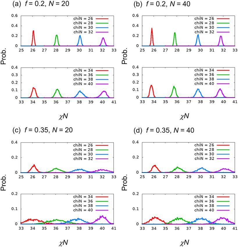
www.nature.com/scientificreports/
Xception42, MobileNet43, and DenseNet44 have been proposed. As a general example, these networks have been
used to estimate the age of a person from a photograph of their face.
According to textbooks and leading p apers45–54, the phase diagram of a block copolymer (BCP) melt is
determined by two independent parameters: χN (where χ is the Flory–Huggins interaction parameter and N
the total number of segments in a BCP chain) and the A-component fraction f. For the A–B diblock copolymer,
N = NA + NB and f = NA /N . Generally, average structures with high symmetries, such as gyroid, cylinder,
lamellar, and sphere phases, have been confirmed via small-angle scattering e xperiments54. Although highly
controlled experiments have achieved high regularities, the actual materials may still have defects and mesoscale
structural distortions. For these highly symmetric structures, such as lamellar structures, domain spacing is
linked with the effective χ parameter55–66. Here, the effective χ parameter is controlled using chemical composition
and chain architecture. The χ value is considered to affect the process of phase separation and characterize the
morphology of the interface. Therefore, it is expected that χ can be estimated from the morphology information
during the phase separation process.
Advanced controls in the phase-separated structure of BCPs are important for industrial applications, such
as directed self-assemblies (DSAs) for semiconductor processes and soft materials such as high-performance
mechanical rubbers. Concerning DSA67–70, regular lamellar and cylindrical structures were required for line/space
arrangements and contact-hole patterning, respectively. The implementation of DSAs on substrates has involved a
rigorous study of nanoimprinting lithography71, electron beam lithography72,73, and solvent-vapor annealing74–76.
Solvent-vapor annealing requires effective interactions among polymers, substrates, and s olvents74–76. To achieve
sub-20 nm periods, the control of high χ parameters with custom chemical synthesis is i mportant77,78. In contrast,
to obtain the optimum mechanical response to the deformation of high-performing soft materials, skillful con-
trols of the “random network of phase-separated domains” frozen in a non-equilibrium state are n eeded79,80. Here,
asymmetric styrene-isoprene-styrene tri-block copolymers were used to obtain industrial materials with high
elasticity and moduli. Morphologies of asymmetric tri-block copolymers have been extensively i nvestigated81–87.
Recently, Aoyagi27 investigated the DL-based predictions of phase d iagrams82. Note that the relationships between
morphologies and mechanical properties under stretching were investigated using coarse-grained molecular
dynamics simulations88–90. Further research on the random network of phase-separated domains governed by
χN is of great interest for the development of high-performing soft materials; estimating χN values from the
observed images is an impactful way to enhance this research. Since analytical approaches were limited for non-
equilibrium states compared to a well phase-separated structures, χN estimation using AI techniques such as
ML and DL is recommended.
The estimation of these two characteristic parameters (χN and f) from cross-sectional images of 3D structures
is desirable for analyzing experimental images. Discrimination of images with different f values is a relatively easy
problem when image sizes are not small because this problem corresponds to the estimation of volume density
from surface density of images. However, it is not clear whether images with the same f value but different χN
values can be discriminated. The problem of estimating χN from images is a simple and fundamental problem
in the experimental science of materials. The interaction parameter, χ is important for understanding the solu-
bility and microphase separation structures of various polymer chains. The value of χN can be experimentally
determined from the correspondence with theoretical prediction by obtaining a highly symmetric structure in
a highly controlled experiment and creating a precise phase diagram54. However, it would be very efficient if χN
could be determined from images of non-equilibrium phase-separated structures, which are easy to observe. In
this study, we investigated the basic relationship between the accuracy and errors of χN estimation.
On one hand, if the relationship between a certain feature of cross-sectional images and estimated χN is
simple (e.g., linear relationship), the interpolation-estimation accuracy is higher for a lower mean absolute
error (MAE) in regression training. On the other hand, if the relationship is not simple, a significantly low
MAE through regression training leads to overfitting, wherein the error in the estimation of χN becomes large.
Herein, we clarify the type of relationship between a certain feature of cross-sectional images and estimated χN.
χN can be estimated from local high-resolution images by observing the concentration gradient at the
interface and/or the interfacial width. Theoretically, the interfacial width is expected to be of the form (χN)−0.5
in the weakly segregated region91. However, there exists a problem: the density-gradient information is lost
owing to staining, which is indispensable for electron-microscope observation, and the binarized image only
contains morphology information. This binarization problem is considered more serious than familiar image
problems such as those related to noise and focus. In this study, we examined the potential of estimating χN
from the morphology information and density profiles in cross-sectional images of global 3D nanostructures
with interfacial width of a small number of pixels. Regarding binarized images of stained specimens observed
via transmission electron microscopy (TEM), an AI technique that performs estimations only from morphology
without a density profile is developed.
Results
Data characterization through Image classification. To generate image data with f = 0.2 and 0.35,
3D field data of the phase-separated structure of A-B BCP were obtained using OCTA/SUSHI92,93 based on
the real-space self-consistent field (SCF) c alculation52,53. Figure 1 shows examples of the images generated for
χN ≥ 25. A lower value of χN was chosen based on the mean field p rediction94 for f = 0.2. We obtained density
fields after convergence of the SCF calculation or 100,000 SCF steps. Although the highly symmetric structure
of triply periodic minimal surface (TPMS) was reported by the experiments, SCF calculations were performed
in this study to obtain “random network of phase-separated domains.” Although cell-size optimization95 is
required to avoid the system-size effect under periodic boundary conditions (PBCs) in case of structures with
high symmetries, this study did not optimize for the same and instead used a PBC box of fixed size. Conceptu-
Scientific Reports | (2021) 11:12322 | https://doi.org/10.1038/s41598-021-91761-8 2
Vol:.(1234567890)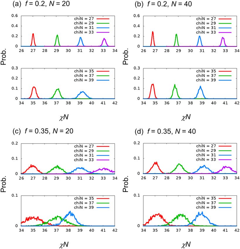
www.nature.com/scientificreports/

                                  Figure 1.  Snapshots of generated structures. (a) 3D isosurface and (b) cross-sectional images.

Scientific Reports |   (2021) 11:12322 |              https://doi.org/10.1038/s41598-021-91761-8                                         3

                                                                                                                                    Vol.:(0123456789)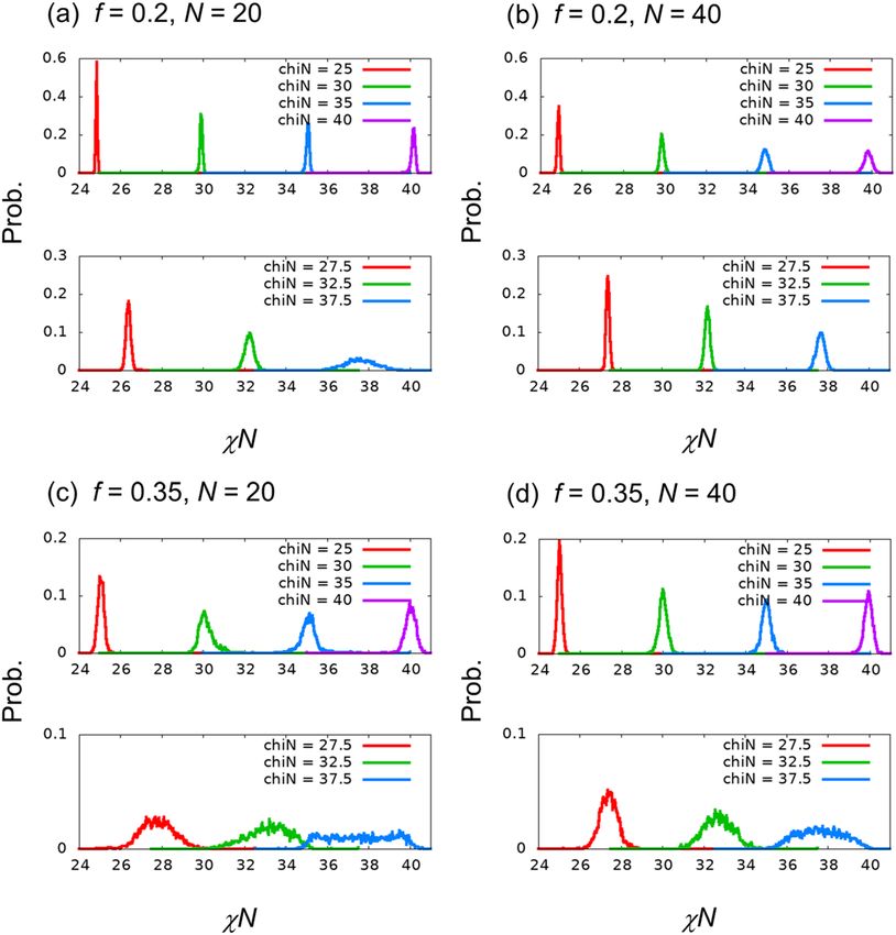
www.nature.com/scientificreports/
ally, it is considered that a highly symmetric structure can be obtained by using a sufficiently large system size or
by optimizing the system size. From another point of view, the images shown in Fig. 1 can be regarded as struc-
tures trapped in the metastable state during the phase separation process. Although these images are not trivial
and have certain complexities, they have features that are governed by the interaction parameter, χN. Although
the highly symmetric structure under TPMS can be classified by a mathematical index such as the Betti number,
there is no mathematical index to classify and express these metastable features. This absence may reveal a case
where ML is difficult but DL may prove to be successful. As a result, these images were considered to be suitable
to evaluate the potential of estimating χN from their morphology information and density profiles.
For understanding the basic characteristics of the examined data system, image classification was performed
before regression. We performed the image classification using Keras96 and TensorFlow97 packages based on the
VGG-16 network. For performance comparison, we performed several ML-based image classifications using
Scikit-learn98. In the ML-based image classifications, we used support vector machine (SVM) with a radial
basis function (rbf) kernel for two features: (1) the histogram of brightness and (2) the histogram of oriented
gradients (HoG). In the DL-based image classifications, binarized images were also examined for comparison.
To summarize, the present work performed the following image classifications:
(1) ML with SVM for histogram of brightness
(2) ML with SVM for HoG features
(3) DL with VGG-16 for binarized images
(4) DL with VGG-16
First, to confirm the superior performance of the VGG-16 model for image classification, we estimated
learning curves until 100 epochs and confusion matrices at 100 epochs. For f = 0.2 and 0.35, and N = 20 and
40, three problems were investigated: (1) 4-class problem with χN = 25, 30, 35, and 40; (2) 6-class problem with
χN = 25, 28, 31, 34, 37, and 40; and (3) 8-class problem with χN = 26, 28, 30, 32, 34, 36, 38, and 40. To avoid
redundancy, results for the 6- and 8-class problems are presented in Section S1 of the Supplementary Information.
Figure 2 shows the learning curves of the trainings performed. We found that 100 epochs are enough to
obtain a reasonable accuracy. Comparisons among f and N suggest that training for f = 0.2 is less difficult than
training for f = 0.35. For f = 0.35, training with N = 20 appears to be more difficult than that with N = 40.
Table 1 presents confusion matrices of the 4-class problem at 100 epochs. For confusion matrix Mi,j , accu-
racy A = i Mi,i / i,j Mi,j and error rate E = 1 − A. For f = 0.2, E = 1.25 × 10⁻⁴ and 0.0 for N = 20 and 40,
respectively. When f = 0.35, E = 1.13 × 10⁻² and 1.63 × 10⁻³ for N = 20 and 40, respectively. It was found
that E for f = 0.2 is lower than that with f = 0.35. This tendency is also found in the 6- and 8-class problems
presented in Section S1 of the Supplementary Information. These behaviors suggest that the images for f = 0.35
are more difficult to learn than for f = 0.2.
The results of the 8-class problem, presented in Section S1of Supplementary Information, suggest that the
accuracy for a larger χN is lower when f = 0.2. This tendency is maintained for (f , N) = (0.35, 20), although it
is not clear for (f , N) = (0.35, 40) because of the large error. This tendency is consistent with that of the 4-class
problem in Table 1. We expect that the accuracy of each class group on χN in the image-classification problems
corresponds to the error of the estimated χN values in the regression problems.
Next, for comparison, we performed ML-based image classifications. Table 2 presents the error rates of the
4-class problem with SVM for the histogram of brightness and the HoG features. Here, 6000 and 2000 images for
each χN class were used for the training and evaluation of generalization ability, respectively. Moreover, DL-based
image-classification results for binarized images are presented for later consideration. The results for the 8-class
problem are also presented in Table 3. The confusion matrices for the 4- and 8-class problems are presented in
Sections S2 and S3 of the Supplementary Information. The DL-based image classification exhibits highly superior
performance (low error rate) compared to that achieved with ML. Therefore, we consider that regression by ML
is not realistic for these datasets. Moreover, it is clear that DL for binarized images outperforms ML.
ML results for the brightness histogram suggest that the prepared images for f = 0.35 are more dependent
on brightness than the images for f = 0.2. The error rate of ML for the HoG feature for these images is worse
than that for the histogram of the brightness. These ML models exhibit inferior performance because the area
of each image is small. The image-classification performance improves for larger image sizes in both ML and DL
models. One of the a uthors99 investigated the effect of image size on generalization ability of image classifica-
tion for morphologies of nanoparticles in rubber matrices, where the morphologies were modeled based on the
ultra-small X-ray scattering s pectrum100.
These image-classification results confirm that the prepared dataset has some features that can be distin-
guished by DL; however, the performance of ML was not good. In the next section, we have used these datasets
for the regression problem in the estimation of the Flory–Huggins χ parameter.
Regression to estimate the Flory–Huggins parameter. As mentioned previously, to investigate the
characteristics of regression to estimate the Flory–Huggins χ parameter, we performed regression using the
VGG-16 model. When preparing training images via electron microscopy for actual materials, such as stained
phased-separated diblock copolymers, the number of prepared materials for the observations is limited to a
small value (e.g., less than a few tens of specimens). Thus, in turn, the number of χN classes is limited to a small
value. Therefore, in the present regression problem, discrete χN rather than continuous χN is used for the train-
ing images. Here, we considered the 8-class problem with training images of χN = 26, 28, 30, 32, 34, 36, 38, and
40. In the classification problem, the generalization ability was evaluated from independent images that belonged
to the same χN classes and were independent of the training images. For the regression problem, two types of
Scientific Reports | (2021) 11:12322 | https://doi.org/10.1038/s41598-021-91761-8 4
Vol:.(1234567890)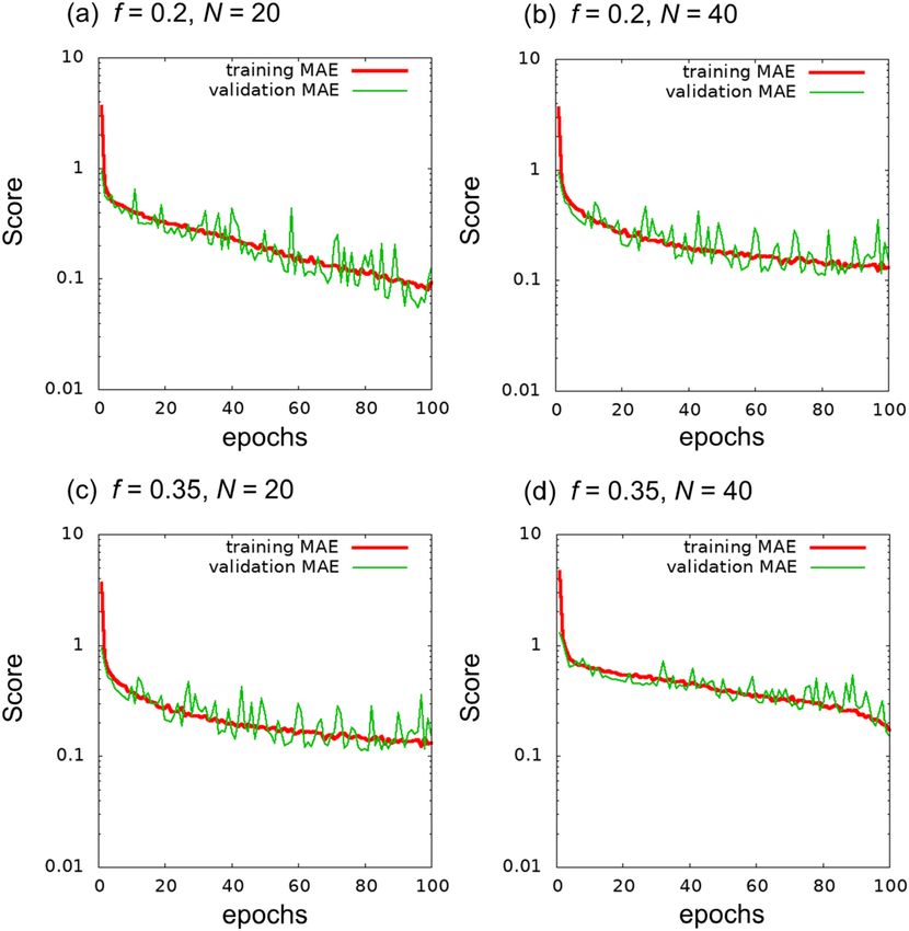
www.nature.com/scientificreports/
Figure 2. Learning curves of the 4-class image classification under training until 100 epochs.
generalization abilities can be evaluated from (1) independent images generated with the same χN value (the
8-classes) and (2) independent images with unlearned χN value. Here, we selected χN = 27, 29, 31, 33, 35, 37,
and 39 as the unlearned χN values. In this study, we evaluated these two generalization abilities.
As a first test, we performed training with 100 epochs. Figure 3 presents the learning curves until 100 epochs.
At f = 0.35, a discrepancy between training MAE and validation MAE was observed, although a similar dis-
crepancy was not observed for f = 0.2. We consider that learning from the given training images was saturated
(i.e., overfitting tendency). In the learning curve of the validation MAE, the trend comprising the minimum and
a subsequent increment can be considered as an indicator of overfitting. In the cases of Fig. 3c and d, the curve
around 60 epochs appears to be the minimum. For comparison with the learned network before overfitting,
we present the results of an independent run with 50 epochs in Section S4 of the Supplementary Information.
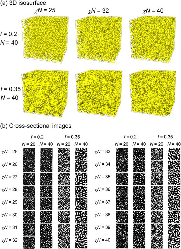
Figure 4 presents distributions of the estimated χN for independent images whose χN values are the same
values as those for the training images. The distribution proceeds differently at f = 0.2 and 0.35. These tenden-
cies are the same as those in the image-classification problem as mentioned in the previous section, and they are
considered to be related to the difficulty encountered in estimating the χN value. The behavior is similar to that
of an independent run with 50 epochs presented in Section S4 of the Supplementary Information.
Table 4 presents the average and standard deviation values of the estimated χN for each χN class. In all cases,
the absolute value of the difference from the true value is approximately 0.1. The standard deviation values are
approximately 0.1–0.2 and 0.2–0.8 for f = 0.2 and 0.35, respectively. The standard deviation values become
larger for larger χN values, as presented in Fig. 4.
Figure 5 and Table 5 present the distribution, average, and standard deviation values of the estimated χN for
independent images of unlearned χN, which are different from those of the training images. We find that the
average of estimated χN for the images with χN = 39 for (f , N) = (0.35, 20) differs from the true χN values
of the images. The difference from the true value is approximately 0.9. The other estimations are found to be as
accurate as the estimations for independent images in the same χN class as the training images. These results
indicate that superior regression estimation is possible for f = 0.2. For f = 0.35, the error is relatively large,
but regression estimation is possible, except for χN > 38 when (f , N) = (0.35, 20). For a detailed investigation
on large χN, see Section S5 of the Supplementary Information, which presents the results of the regression for
χN = 36.5, 37.5, 38.5, and 39.5 and the image classification of the 3-class problem with χN = 38, 39, and 40.
Scientific Reports | (2021) 11:12322 | https://doi.org/10.1038/s41598-021-91761-8 5
Vol.:(0123456789)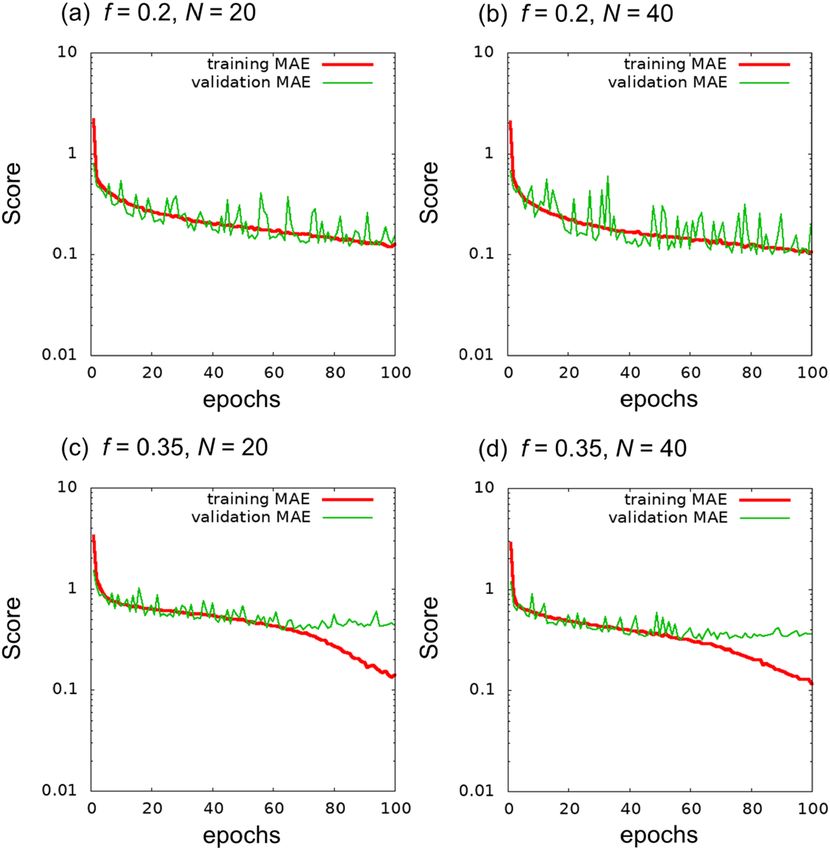
www.nature.com/scientificreports/
Estimated χN class
(a) f = 0.2, N = 20 25 30 35 40
χN = 25 2000 0 0 0
χN = 30 0 2000 0 0
Actual
χN = 35 0 0 1999 1
χN = 40 0 0 0 2000
Estimated χN class
(b) f = 0.2, N = 40 25 30 35 40
χN = 25 2000 0 0 0
χN = 30 0 2000 0 0
Actual
χN = 35 0 0 2000 0
χN = 40 0 0 0 2000
Estimated χN class
(c) f = 0.35, N = 20 25 30 35 40
χN = 25 1985 15 0 0
χN = 30 0 1967 33 0
Actual
χN = 35 1 2 1966 31
χN = 40 0 0 8 1992
Estimated χN class
(d) f = 0.35, N = 40 25 30 35 40
χN = 25 1999 1 0 0
χN = 30 2 1997 1 0
Actual
χN = 35 0 2 1992 6
χN = 40 0 0 1 1999
Table 1. Confusion matrices of the 4-class problem at 100 epochs.
f = 0.2 f = 0.35
N = 20 N = 40 N = 20 N = 40
(1) ML-based for histogram of brightness 0.525 0.512 0.150 0.254
(2) ML-based for HoG features 0.512 0.748 0.545 0.612
(3) DL-based for binarized images 0.134 0.137 0.168 0.251
(4) DL-based 1.25 × 10⁻⁴ 0.0 1.13 × 10⁻² 1.63 × 10⁻³
Table 2. Error rates for image classification for the 4-class problem.
f = 0.2 f = 0.35
N = 20 N = 40 N = 20 N = 40
(1) ML-based for histogram of brightness 0.763 0.757 0.299 0.387
(2) ML-based for HoG features 0.719 0.721 0.791 0.805
(3) DL-based for binarized images 0.455 0.442 0.515 0.515
(4) DL-based 2.50 × 10⁻⁴ 4.94 × 10⁻⁴ 1.46 × 10⁻² 1.09 × 10⁻²
Table 3. Error rates for image classification for the 8-class problem.
Cases with long learning times and transfer learning. In some cases, to obtain small MAEs, long
learning times (epochs) and/or transfer learning are applied. In this study, we also attempted to perform learn-
ing with large epochs and transfer learning. However, both the cases showed overfitting and poor generalization
ability. The detailed results are presented in Sections S6–S9 of the Supplementary Information.
These results indicate that it is a realistic solution to use a trained network, wherein overfitting does not occur
in the generalization-ability evaluation of the unlearned χN.
Confirmation for the binarized images. To confirm the effects of interfacial density gradients on the
regression problem and feasibility of χN estimation for stained specimens, we investigated the regression per-
Scientific Reports | (2021) 11:12322 | https://doi.org/10.1038/s41598-021-91761-8 6
Vol:.(1234567890)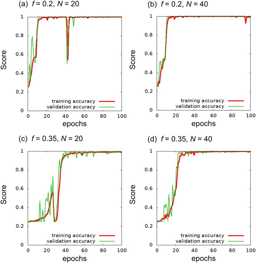
www.nature.com/scientificreports/

                                  Figure 3.  Learning curves of the regression problem until 100 epochs.

                                  formance for binarized images. Tables 6 and 7 present the average and standard deviation values of the estimated
                                  χN for each χN class, as detailed in Section S10 of the Supplementary Information. We consider that DL-based
                                  χN estimation for binarized images is learning the characteristics of morphology in the binary images without
                                  density gradients. The distributions of the estimated χN for the binarized images are much wider than those for
                                  the gray-scale images. Absolute differences from the true values of χN are also larger than those for the gray-
                                  scale images. Therefore, we conclude that the gray-scale images have essential information for χN estimation.
                                  This suggests that χN can be evaluated accurately without using DL if an arithmetic calculation method for
                                  estimating χN from a cross-sectional image is developed. However, at present, such a method is unknown; thus,
                                  DL is an effective tool.
                                      It should be noted that the χN estimation for the binarized image is predictable as an average, although the
                                  error is large. In TEM observations of polymer materials, staining such as by OsO4 is currently essential owing
                                  to the limited detector ability. The observed images of the stained sample are considered to correspond to the
                                  binarized images. The confirmation that the binarized image has a certain estimation ability is useful information
                                  in the future analysis of TEM images of the actual materials.

                                  Comparison with regression with the 4‑class training images. To clarify the effects of the number
                                  of classes and step size of χN on the error, we investigated the cases of training using the 4-class training images
                                  with χN = 25, 30, 35, and 40. Figure 6 shows the learning curves for the 4-class training images. The MAEs at
                                  100 epochs in the 4-class problem were smaller than those in the 8-class problem.
                                       Figure 7 presents the distribution of the estimated χN for the 4-class problem. Except for the cases of
                                  (f , N) = (0.2, 40), we find that there is no discriminating ability for χN = 37.5. In particular, for the cases of
                                  (χN, f , N) = (37.50.35, 20), we find sharp peaks at χN = 35 and 40 which were χN values of the training images
                                  as shown in Fig. 7c. These peaks at the χN values of the training data are typical behaviors of overfitting, as
                                  observed in Section S7 of the Supplementary Information.
                                       Except for the large χN, it was found that the estimation with the 4-class training images was as accurate
                                  as that with the 8-class training images. This finding is supported by the behaviors of the average and standard
                                  deviation values presented in Table 8. We consider that this knowledge is useful in the analysis of actual experi-
                                  mental images.

Scientific Reports |   (2021) 11:12322 |               https://doi.org/10.1038/s41598-021-91761-8                                                   7

                                                                                                                                               Vol.:(0123456789)
www.nature.com/scientificreports/
Figure 4. Probability distribution functions of the estimated χN value for evaluation data generated with same
χN values as the teaching data. Here, the size of each bin was 0.05.
(f, N) = (0.2, 20) (f, N) = (0.2, 40) (f, N) = (0.35, 20) (f, N) = (0.35, 40)
χN = 26 26.084 ± 0.061 25.850 ± 0.055 26.130 ± 0.239 26.105 ± 0.221
χN = 28 28.081 ± 0.089 27.831 ± 0.069 28.083 ± 0.430 28.113 ± 0.325
χN = 30 30.094 ± 0.100 29.826 ± 0.089 30.097 ± 0.493 30.151 ± 0.370
χN = 32 32.094 ± 0.128 31.804 ± 0.100 32.073 ± 0.591 32.146 ± 0.439
χN = 34 34.120 ± 0.149 33.812 ± 0.118 34.100 ± 0.708 34.186 ± 0.479
χN = 36 36.139 ± 0.190 35.768 ± 0.139 36.139 ± 0.795 36.219 ± 0.544
χN = 38 38.139 ± 0.251 37.837 ± 0.182 37.776 ± 0.678 38.120 ± 0.561
χN = 40 40.127 ± 0.227 39.732 ± 0.183 39.883 ± 0.594 39.926 ± 0.510
Table 4. Averages and standard deviations of estimated χN for each χN class, which is the same for the
teaching images.
Summary and discussion
DL-based methods were studied to estimate the Flory–Huggins χ parameter of A–B diblock copolymers from
2D cross-sectional images generated from SCF calculations, assuming them to observation images from electron
microscopes. In this study, we aimed to estimate χN for images created by a particular process. Note that χN esti-
mation, independent of the material processes, cannot be discussed because we used only one image-generation
method in this study. Through SCF calculations, 10,000 images for each χN were obtained from cross-sectional
views of the 3D phase-separated structures in random directions at randomly selected positions. Here, the 3D
density field data were obtained by real-space SCF simulations in the 25–40 χN range for f = 0.2 and 0.35 and
N = 20 and 40. For DL, we used VGG-1638.
Scientific Reports | (2021) 11:12322 | https://doi.org/10.1038/s41598-021-91761-8 8
Vol:.(1234567890)www.nature.com/scientificreports/
Figure 5. Probability distribution functions of the estimated χN for evaluation data generated with unlearned
χN values.
(f, N) = (0.2, 20) (f, N) = (0.2, 40) (f, N) = (0.35, 20) (f, N) = (0.35, 40)
χN = 27 27.032 ± 0.081 26.818 ± 0.063 26.976 ± 0.379 27.029 ± 0.293
χN = 29 29.087 ± 0.092 28.843 ± 0.079 29.088 ± 0.457 29.101 ± 0.348
χN = 31 31.090 ± 0.120 30.824 ± 0.095 31.093 ± 0.560 31.189 ± 0.410
χN = 33 33.114 ± 0.138 32.821 ± 0.111 33.072 ± 0.626 33.151 ± 0.465
χN = 35 35.112 ± 0.171 34.799 ± 0.130 35.113 ± 0.771 35.187 ± 0.522
χN = 37 37.103 ± 0.216 36.725 ± 0.157 37.076 ± 0.741 37.173 ± 0.565
χN = 39 39.254 ± 0.295 38.885 ± 0.182 38.114 ± 0.529 38.962 ± 0.502
Table 5. Averages and standard deviations of estimated χN values for each unlearned χN.
To show that the generated images can be classified systematically, DL-based image classification was per-
formed. The accuracy for f = 0.2 was found to be better than that for f = 0.35 because of the difficulty encoun-
tered in distinguishing owing to the resemble images. It was clarified that the accuracy for a larger χN is lower
when f = 0.35.
In addition, we investigated image classification performance of ML with SVM for the histogram of brightness
and the HoG features as well as DL for binarized images. The error rates of ML were considerably larger than
those of DL. Thus, regression via ML was found to be difficult for these prepared datasets. We also confirmed that
the image classification performance by DL for binary images was inferior to those for gray-scale images. The
binarization also affected the regression performance. In addition, we found that the DL-based χN estimation
for the binarized image was predictable as an average, although the error was large. This is an important finding
to extend χN estimation for images in TEM observations of stained polymer materials.
Scientific Reports | (2021) 11:12322 | https://doi.org/10.1038/s41598-021-91761-8 9
Vol.:(0123456789)www.nature.com/scientificreports/
(f, N) = (0.2, 20) (f, N) = (0.2, 40) (f, N) = (0.35, 20) (f, N) = (0.35, 40)
χN = 26 26.232 ± 0.548 26.409 ± 0.898 27.229 ± 1.462 28.680 ± 1.761
χN = 28 28.241 ± 1.009 28.230 ± 1.238 29.589 ± 2.224 29.274 ± 1.909
χN = 30 30.572 ± 1.511 30.515 ± 1.546 31.547 ± 2.466 29.911 ± 1.955
χN = 32 32.807 ± 1.871 32.750 ± 1.753 33.125 ± 2.342 31.363 ± 2.133
χN = 34 34.746 ± 1.967 34.521 ± 1.750 34.124 ± 2.342 33.286 ± 2.156
χN = 36 36.330 ± 1.873 35.777 ± 1.795 34.864 ± 2.297 35.836 ± 1.832
χN = 38 37.211 ± 1.792 36.928 ± 1.876 35.076 ± 2.220 37.545 ± 1.400
χN = 40 38.005 ± 1.661 38.322 ± 1.871 37.855 ± 2.099 39.451 ± 1.043
Table 6. Averages and standard deviations of estimated χN for each χN class for the binarized images. Here,
the χN class was same value of the teaching image.
(f, N) = (0.2, 20) (f, N) = (0.2, 40) (f, N) = (0.35, 20) (f, N) = (0.35, 40)
χN = 27 27.067 ± 0.772 27.261 ± 1.106 28.288 ± 1.946 28.615 ± 1.749
χN = 29 29.386 ± 1.281 29.485 ± 1.441 30.605 ± 2.375 29.143 ± 1.817
χN = 31 31.640 ± 1.672 31.728 ± 1.631 32.512 ± 2.449 30.660 ± 2.126
χN = 33 33.908 ± 1.925 33.801 ± 1.696 33.593 ± 2.352 32.340 ± 2.151
χN = 35 35.363 ± 1.962 35.190 ± 1.774 34.526 ± 2.284 34.552 ± 2.005
χN = 37 36.745 ± 1.855 36.476 ± 1.768 34.956 ± 2.208 36.712 ± 1.668
χN = 39 37.637 ± 1.741 37.577 ± 1.834 35.328 ± 2.101 38.415 ± 1.058
Table 7. Averages and standard deviations of estimated χN for each unlearned χN class for the binarized
images.
We performed DL of regression problems based on the VGG-16 network model. For the 8-class problem,
χN was set at 26, 28, 30, 32, 34, 36, 38, and 40. To evaluate the generalization ability, MAEs for the following two
image groups were estimated: (1) independent images generated with the same χN value as that for the training
images and (2) independent images with unlearned χN value such as χN = 27, 29, 31, 33, 35, 37, and 39.
We investigated the distribution of the estimated χN of independent images with the unlearned χN values.
Large χN values could not be accurately estimated, which can be ascribed to the difficulty encountered in image
classification. For (f , N) = (0.35, 20), the image classification for the 3-class problem for χN = 38, 39, and 40
failed to distinguish images for χN = 38 and 39. Except when χN was large, we obtained accurate average values
of χN for the examined images, and the standard deviation was approximately 0.1 and 0.5 for f = 0.2 and 0.35,
respectively. To improve the accuracy of estimation for large χN, we require high-resolution images wherein
the density gradient at the phase-separation interface can be recognized. Studies in this direction, including
experimental observation data, are underway.
Moreover, we found that the learning performances for the 4-class problem were comparable to those for the
8-class problem except when χN was large. This information is useful for the analysis of experimental image data.
On the other hand, given that the estimation with the 8-class teacher dataset was more accurate than that with
the 4-class dataset, the performance could be improved with the incorporation of smaller χN intervals into the
teacher data. For example, it is difficult to prepare specimens that have a wide χN range with 0.1 intervals even
in simulations; however, it may not be impossible. Research that provides insights into how small an χN interval
is required for more accurate estimations, would be an important next step in this field.
To estimate χN from experimental images, in addition to the effects of binarization associated with observa-
tions of stained specimens, we should train a regression network model that is robust to the effects of noise and
image adjustments (including focus) of experimental data. To investigate random local noises and variations in
image contrast and brightness, a large amount of experimental image data must be analyzed and pseudo image
data must be generated accordingly. Recently developed electron-microscope automation techniques can be
applied to observe a large area of images from one stained specimen at one observation. Research in these direc-
tions is also being conducted.
In this study, we considered images created solely from a particular process of phase separations. This limits
our ability to estimate χN only for that specific material process. Although the effectiveness of the learned net-
work was limited to a specific process, we expected the estimation ability of the physical parameters governing
phase-separation to be utilizable not only for polymers but also for metals. In the research and development of
real materials, χN is expected to be estimated from structures obtained from various material processes. Further
prospects in this field include an investigation into the feasibility of χN estimation, independent of material
processes.
Scientific Reports | (2021) 11:12322 | https://doi.org/10.1038/s41598-021-91761-8 10
Vol:.(1234567890)www.nature.com/scientificreports/
Figure 6. Learning curves of the regression problem with the 4-class teaching images.
Methods
Image data preparation through SCF calculation. For f = 0.2 and 0.35, 3D field data of the phase-
separated structure of A-B BCP were obtained using the OCTA/SUSHI p ackage92,93 based on the real-space SCF
52,53
calculation . The theoretical background is briefly explained in Section S11 of the Supplementary Informa-
tion. The system size was set at 128 × 128 × 128 under PBCs, and a regular 128 × 128 × 128 grid mesh was used. In
the present study, the following cases were examined:N = 20 and 40. According to the mean field p rediction94,
the boundary value, χN, of the order–disorder phase transition is approximately 23.5 for f = 0.2 and 12.5 for
f = 0.35. Thus, we generated images for χN ≥ 25, as presented in Fig. 1. In practice, we obtained the 3D field
data with an χN interval of 0.5.
All the images were obtained from cross-sectional views of the 3D density field data of the A domain in ran-
dom directions at randomly selected positions. A total of 10,000 input images with 64 × 64 pixels were prepared
for each class. In generating a cross-sectional view with 64 × 64 pixels from 3D field data of 128 × 128 × 128 grids
under the PBCs, we performed linear-weight interpolation. Here, the images were 8-bit gray-scale images. We
placed the same data in 3 RGB channels for generality in preliminarily tests such as transfer learning using the
weight data trained by ImageNet38. Learning with the same data on three channels did not have any significant
effect, except for a slight difference in convergence behaviors.
This differs from the method of obtaining highly symmetric structures from SCF calculations. To construct
ordered structures in the shape of lamellae, cylinders, and gyroids, artificial initial estimate and cell-size optimiza-
tion—a parameter search of the box size to minimize the free e nergy95—are effective. The initial value and search
range are important to obtain a reasonable solution. If we start from uniformly mixed initial states, hydrodynamic
effects are essential to obtain ordered s tructures101. By contrast, to obtain random network of phase-separated
domains, spatially uncorrelated fields were used as initial density profiles and cell-size optimization was not used.
Image classification by DL. In the image-classification problem, the labels of the training images are
learned and the trained model outputs the estimated probability of each label for an arbitrary image. CNNs are
well known to have high image-classification a bility38–44. Keras96 provides all popular network models for image
classification including VGG-16 model, which is one of the more successful CNN models. Comparisons among
popular network models provided by K eras96 are presented in Section S12 of the Supplementary Information.
Scientific Reports | (2021) 11:12322 | https://doi.org/10.1038/s41598-021-91761-8 11
Vol.:(0123456789)www.nature.com/scientificreports/
Figure 7. Probability distribution functions of the estimated χN for evaluation data for the 4-class teaching
images.
(f, N) = (0.2, 20) (f, N) = (0.2, 40) (f, N) = (0.35, 20) (f, N) = (0.35, 40)
χN = 25 24.852 ± 0.032 24.875 ± 0.056 25.062 ± 0.184 25.006 ± 0.111
χN = 30 29.910 ± 0.066 29.876 ± 0.102 30.183 ± 0.436 30.004 ± 0.210
χN = 35 35.064 ± 0.083 34.865 ± 0.163 35.145 ± 0.639 35.011 ± 0.277
χN = 40 40.161 ± 0.104 39.845 ± 0.186 40.004 ± 0.414 39.925 ± 0.270
χN = 27.5 26.385 ± 0.115 27.387 ± 0.079 27.797 ± 0.796 27.401 ± 0.417
χN = 32.5 32.236 ± 0.224 32.201 ± 0.137 33.155 ± 1.031 32.704 ± 0.704
χN = 37.5 37.594 ± 0.727 37.677 ± 0.200 37.563 ± 1.540 37.622 ± 1.071
Table 8. Averages and standard deviations of estimated χN values for each χN in the 4-class problem.
The VGG-16 model has 16 layers, including five convolutional blocks (13 convolutional layers), as shown in
Fig. 8.
To determine the parameters of the VGG-16 model, we used T ensorFlow97 as the backend for Keras. For
image classification, 6000 and 2000 images per χN class were used as training and testing images, respectively,
for the learning and for evaluating the generalization ability. The stochastic gradient descent (SGD) method was
used as the optimizer for the classification problem; a standard learning rate of 10–4 and momentum 0.9 was
used for simplicity.
Estimation (regression) of the Flory–Huggins parameter via DL. In the regression problem, the
values of the training images are learned and the trained model outputs the estimated values for an arbitrary
image. For the regression problem, we used a network based on the VGG-16 model, as presented in Fig. 8b.
Compared to the classification problem, in the regression problem, the last block is different, as shown in Fig. 8.
Scientific Reports | (2021) 11:12322 | https://doi.org/10.1038/s41598-021-91761-8 12
Vol:.(1234567890)www.nature.com/scientificreports/
Figure 8. Schematic images of network architectures for (a) image-classification problem and (b) regression
problem based on the VGG-16 model. The first five convolutional blocks are the same, but the last block is
different. For the image-classification problem, the output is a vector whose number of elements equals the
number of classes. For the regression problem, the output is a scalar. Here, the numbers at the lower right of
each block denote the number of elements of the output tensor of each block.
In the regression problem, we used the adaptive moment estimation (Adam)102 as the optimizer, with a standard
learning rate of 10–6 and (β1 , β2 ) = (0.9, 0.999) for simplicity.
Data availability
All generated image data used are available from the corresponding author upon reasonable request.
Received: 28 March 2021; Accepted: 31 May 2021
References
1. LeCun, Y., Bengio, Y. & Hinton, G. Deep learning. Nature 521, 436–444 (2015).
2. Schmidhuber, J. Deep learning in neural networks: An overview. Neural Netw. 61, 85–117 (2015).
3. Hinton, G. E. & Salakhutdinov, R. Reducing the dimensionality of data with neural networks. Science 313, 504–507 (2006).
4. Russakovsky, O. et al. Imagenet large scale visual recognition challenge. Int. J. Comput. Vis. 115, 211–252 (2015).
5. Bojarski, M. et al. End to end learning for self-driving cars. http://arxiv.org/abs/1604.07316 (2016).
6. Silver, D. et al. Mastering the game of Go with deep neural networks and tree search. Nature 529, 484–489 (2016).
7. Cho, A. AI systems aim to sniff out coronavirus outbreaks. Science 368, 810–811 (2020).
8. Mei, X. et al. Artificial intelligence–enabled rapid diagnosis of patients with COVID-19. Nat. Med. 26, 1224–1228 (2020).
9. Ardakani, A. A., Kanafi, A. R., Acharya, U. R., Khadem, N. & Mohammadi, A. Application of deep learning technique to manage
COVID-19 in routine clinical practice using CT images: results of 10 convolutional neural networks. Comput. Biol. Med. 121,
103795 (2020).
10. Ramprasad, R., Batra, R., Pilania, G., Mannodi-Kanakkithodi, A. & Kim, C. Machine learning in materials informatics: recent
applications and prospects. NPJ Comput. Mater. 3, 54 (2017).
11. Schmidt, J., Marques, M. R. G., Botti, S. & Marques, M. A. L. Recent advances and applications of machine learning in solid-state
materials science. NPJ Comput. Mater. 5, 83 (2019).
12. Chen, C.-T. & Gu, G. X. Machine learning for composite materials. MRS Commun. 9, 556–566 (2019).
13. Kumar, J. K., Li, Q. & Jun, Y. Challenges and opportunities of polymer design with machine learning and high throughput
experimentation. MRS Commun. 9, 537–544 (2019).
14. Jackson, N. E., Webb, M. A. & de Pablo, J. J. Recent advances in machine learning towards multiscale soft materials design. Curr.
Opin. Chem. Eng. 23, 106–114 (2019).
15. Hansoge, N. K. et al. Materials by design for stiff and tough hairy nanoparticle assemblies. ACS Nano 12, 7946–7958 (2018).
16. Doi, H., Takahashi, K. Z., Tagashira, K., Fukuda, J. & Aoyagi, T. Machine learning-aided analysis for complex local structure of
liquid crystal polymers. Sci. Rep. 9, 1–12 (2019).
17. Kajita, S., Kinjo, T. & Nishi, T. Autonomous molecular design by Monte-Carlo tree search and rapid evaluations using molecular
dynamics simulations. Commun. Phys. 45, 77 (2020).
18. Wu, S. et al. Machine-learning-assisted discovery of polymers with high thermal conductivity using a molecular design algorithm.
NPJ Comput. Mater. 5, 66 (2019).
Scientific Reports | (2021) 11:12322 | https://doi.org/10.1038/s41598-021-91761-8 13
Vol.:(0123456789)www.nature.com/scientificreports/
19. Kumar, J. N. et al. Machine learning enables polymer cloud-point engineering via inverse design. NPJ Comput. Mater. 5, 73
(2019).
20. Agrawal, A. & Choudhary, A. Deep materials informatics: Applications of deep learning in materials science. MRS Commun.
9, 779–792 (2019).
21. Azimi, S. M., Britz, D., Engstler, M., Fritz, M. & Mücklich, F. Advanced steel microstructural classification by deep learning
methods. Sci. Rep. 8, 2128 (2018).
22. Zhang, Y. & Ngan, A. H. W. Extracting dislocation microstructures by deep learning. Int. J. Plast. 115, 18–28 (2019).
23. Roberts, G. et al. Deep learning for semantic segmentation of defects in advanced STEM images of steels. Sci. Rep. 9, 12744
(2019).
24. Stan, T., Thompson, Z. T. & Voorhees, P. W. Optimizing convolutional neural networks to perform semantic segmentation on
large materials imaging datasets: X-ray tomography and serial sectioning. Mat. Char. 160, 110119 (2020).
25. Jablonka, K. M., Ongari, D., Moosavi, S. M. & Smit, B. Big-data science in porous materials: Materials genomics and machine
learning. Chem. Rev. 120(16), 8066–8129 (2020).
26. DeCost, B. L., Lei, B., Francis, T. & Holm, E. A. High throughput quantitative metallography for complex microstructures using
deep learning: A case study in ultrahigh carbon steel. Microsc. Microanal. 25, 21–29 (2019).
27. Aoyagi, T. Deep learning model for predicting phase diagrams of block copolymers. Comput. Mater. Sci. 188, 110224 (2021).
28. Hagita, K., Higuchi, T. & Jinnai, H. Super-resolution for asymmetric resolution of FIB-SEM 3D imaging using AI with deep
learning. Sci. Rep. 8, 5877 (2018).
29. Wang, Y., Teng, Q., He, X., Feng, J. & Zhang, T. CT-image of rock samples super resolution using 3D convolutional neural
network. Comput. Geo. 133, 104314 (2019).
30. Kamrava, S., Tahmasebi, P. & Sahimi, M. Enhancing images of shale formations by a hybrid stochastic and deep learning algo-
rithm. Neural Netw. 118, 310–320 (2019).
31. Liu, Y. et al. General resolution enhancement method in atomic force microscopy using deep learning. Adv. Theor. Simul. 2,
1800137 (2019).
32. Liu, Y., Yu, B., Liu, Z., Beck, D. & Zeng, K. High-speed piezoresponse force microscopy and machine learning approaches for
dynamic domain growth in ferroelectric materials. ACS Appl. Mater. Interfaces 12, 9944–9952 (2020).
33. Wang, C., Ding, G., Liu, Y. & Xin, H. L. 0.7 Å resolution electron tomography enabled by deep-learning-aided information
recovery. Adv. Intel. Sys. 1, 2000152 (2020).
34. Hiraide, K., Hirayama, K., Endo, K. & Muramatsu, M. Application of deep learning to inverse design of phase separation structure
in polymer alloy. Comput. Mater. Sci. 190, 110278 (2021).
35. Spontak, R. J., Williams, M. C. & Agard, D. A. Three-dimensional study of cylindrical morphology in a styrene-butadiene-styrene
block copolymer. Polymer 29, 387–395 (1988).
36. Jinnai, H. & Spontak, R. J. Transmission electron microtomography in polymer research. Polymer 50, 1067–1087 (2009).
37. Jinnai, H., Spontak, R. J. & Nishi, T. Transmission electron microtomography and polymer nanostructures. Macromolecules 43,
1675–1688 (2010).
38. Krizhevsky, A., Sutskever, I. & Hinton, G. ImageNet classification with deep convolutional neural networks. Adv. Neural Inf.
Process. Syst. 25, 1106–1114 (2012).
39. Simonyan, K. & Zisserman, A. Very Deep Convolutional Networks for Large-Scale Image Recognition. Proc. Int. Conf. Learn.
Represent. (2015). http://arxiv.org/abs/1409.1556.
40. He, K., Zhang, X., Ren, S. & Sun, J. Deep residual learning for image recognition. Proc. IEEE Conf. Comp. Vis. Patt. Recogn.
770–778 (2016).
41. Szegedy, C. et al. Going deeper with convolutions. Proc. IEEE Conf. Comp. Vis. Patt. Recogn. 1–9 (2015).
42. Chollet, F. Xception: Deep learning with depthwise separable convolutions. Proc. IEEE Conf. Comp. Vis. Patt. Recogn. 1251–1258
(2017).
43. Sandler, M., Howard, A., Zhu, M., Zhmoginov, A. & Chen, L.-C. Mobilenetv2: inverted residuals and linear bottlenecks. Proc.
IEEE Conf. Comp. Vis. Patt. Recogn. 4510–4520 (2018).
44. Huang, G., Liu, Z., van der Maaten, L. & Weinberger, K. Q. Densely connected convolutional networks. Proc. IEEE Conf. Comp.
Vis. Patt. Recogn. 4700–4708 (2017).
45. Doi, M. Introduction to Polymer Physics (Clarendon Press, 1996).
46. Fredrickson, G. H. The Equilibrium Theory of Inhomogeneous Polymers (Clarendon Press, 2006).
47. Matsen, M. W. & Bates, F. S. Unifying weak- and strong-segregation block copolymer theories. Macromolecuels 29, 1091–1098
(1996).
48. Hajduk, D. A. et al. The gyroid: A new equilibrium morphology in weakly segregated diblock copolymers. Macromolecules 27,
4063–4075 (1994).
49. Jinnai, H. et al. Direct measurement of interfacial curvature distributions in a bicontinuous block copolymer morphology. Phys.
Rev. Lett. 84, 518–521 (2000).
50. Bates, M. W. et al. Stability of the A15 phase in deblock copolymer melts. Proc. Natl. Acad. Sci. USA 116, 13194–13199 (2019).
51. Uneyama, T. & Doi, M. Density functional theory for block copolymer melts and blends. Macromolecules 38, 196–205 (2005).
52. Matsen, M. W. & Schick, M. Stable and unstable phases of a diblock copolymer melt. Phys. Rev. Lett. 72, 2660–2663 (1994).
53. Kawakatsu, T. Statistical Physics of Polymers: An Introduction (Springer, 2004).
54. Khandpur, A. K. et al. Polyisoprene-polystyrene diblock copolymer phase diagram near the order-disorder transition. Macro-
molecules 28, 8796–8806 (1995).
55. Milner, S. T. Chain architecture and asymmetry in copolymer microphases. Macromolecules 27, 2333–2335 (1994).
56. Matsushita, Y. & Noda, I. Morphology and domain size of a model graft copolymer. Macromol. Symp. 106, 251–257 (1996).
57. Matsushita, Y., Noda, I. & Torikai, N. Morphologies and domain sizes of microphase-separated structures of block and graft
copolymers of different types. Macromol. Symp. 124, 121–133 (1997).
58. Poelma, J. et al. Cyclic block copolymers for controlling feature sizes in block copolymer lithography. ACS Nano 6, 10845–10854
(2012).
59. Isono, T. et al. Sub-10 nm nano-organization in AB2- and AB3-type miktoarm star copolymers consisting of maltoheptaose and
polycaprolactone. Macromolecules 46, 1461–1469 (2013).
60. Pitet, L. M. et al. Well-organized dense arrays of nanodomains in thin-films of poly(dimethylsiloxane)-b-poly(lactide) diblock
copolymers. Macromolecules 46, 8289–8295 (2013).
61. Shi, W. et al. Producing small domain features using miktoarm block copolymers with large interaction parameters. ACS Macro
Lett. 4, 1287–1292 (2015).
62. Minehara, H. et al. Branched block copolymers for tuning of morphology and feature size in thin film nanolithography. Mac-
romolecules 49, 2318–2326 (2016).
63. Sun, Z. et al. Using block copolymer architecture to achieve sub-10 nm periods. Polymer 121, 297–303 (2017).
64. Isono, T. et al. Microphase separation of carbohydrate-based star-block copolymers with sub-10 nm periodicity. Polym. Chem.
10, 1119–1129 (2019).
Scientific Reports | (2021) 11:12322 | https://doi.org/10.1038/s41598-021-91761-8 14
Vol:.(1234567890)www.nature.com/scientificreports/
65. Goodson, A. D., Troxler, J. E., Rick, M. S., Ashbaugh, H. S. & Albert, J. N. L. Impact of cyclic block copolymer chain architec-
ture and degree of polymerization on nanoscale domain spacing: A simulation and scaling theory analysis. Macromolecule 52,
9389–9397 (2019).
66. Hagita, K., Honda, T., Murashima, T. & Kawakatsu, T. Lamellar domain spacing of diblock copolymers of ring and 4-arm star -
real-space self consistent field method versus dissipative particle dynamics simulation. In preparation.
67. Jeong, S.-J., Kim, J. Y., Kim, B. H., Moon, H.-S. & Kim, S. O. Directed self-assembly of block copolymers for next generation
nanolithography. Mater. Today 16, 468–476 (2013).
68. Morris, M. A. Directed self-assembly of block copolymers for nanocircuitry fabrication. Microelectron. Eng. 132, 207–217 (2015).
69. Rasappa, S. et al. High quality sub-10 nm graphene nanoribbons by on-chip PS-b-PDMS block copolymer lithography. RSC
Adv. 5, 66711–66717 (2015).
70. Cummins, C. & Morris, M. A. Using block copolymers as infiltration sites for development of future nanoelectronic devices:
Achievements, barriers, and opportunities. Microelectron. Eng. 195, 74–85 (2018).
71. Traub, M. C., Longsine, W. & Truskett, V. N. Advances in nanoimprint lithography. Annu. Rev. Chem. Biomolec. Eng. 7, 583–604
(2016).
72. Chen, Y. Nanofabrication by electron beam lithography and its applications. Microelectron. Eng. 135, 57–72 (2015).
73. Gangnaik, A. S., Georgiev, Y. M. & Holmes, J. D. New generation electron beam resists: A review. Chem. Mater. 29(5), 1898–1917
(2017).
74. Selkirk, A. et al. Optimization and control of large block copolymer self-assembly via precision solvent vapor annealing. Mac-
romolecules 54, 1203–1215 (2021).
75. Rasappa, S. et al. Morphology evolution of PS-b-PDMS block copolymer and its hierarchical directed self-assembly on block
copolymer templates. Microelectron. Eng. 192, 1–7 (2018).
76. Ghoshal, T., Holmes, J. D. & Morris, M. A. Development of ordered, porous (sub-25 nm dimensions) surface membrane struc-
tures using a block copolymer approach. Sci. Rep. 8, 7252 (2018).
77. Bates, C. M. et al. Polarity-switching top coats enable orientation of sub-10-nm block copolymer domains. Science 338, 775–779
(2012).
78. Otsuka, I. et al. 10 nm scale cylinder-cubic phase transition induced by caramelization in sugar-based block copolymers. ACS
Macro Lett. 1, 1379–1382 (2012).
79. Takayanagi, A. et al. Relationship between microphase separation structure and physical property of thermoplastic elastomer
mixtures. Koubunshi Ronbunshu 72(3), 104–109 (2015) (In Japanese).
80. Takayanagi, A. & Honda, T. Structure analyses of the mixture of thermoplastic elastomers having different symmetry in stretch-
ing process. Nippon Gomu Kyokaishi 92, 148–151 (2019) (In Japanese).
81. Matsen, M. W. & Thompson, R. B. Equilibrium behavior of symmetric ABA triblock copolymer melts. J. Chem. Phys. 111, 7139
(1999).
82. Matsen, M. W. Equilibrium behavior of asymmetric ABA triblock copolymer melts. J. Chem. Phys. 113, 5539 (2000).
83. Matsen, M. W. The standard Gaussian model for block copolymer melts. J. Phys. 14, R21–R47 (2002).
84. Adhikari, R., Huy, T. A., Buschnakowski, M., Michler, G. H. & Knoll, K. Asymmetric PS- block -(PS-co-PB)- block -PS block
copolymers: morphology formation and deformation behaviour. New J. Phys. 6, 28–28 (2004).
85. Smith, S. D., Hamersky, M. W., Bowman, M. K., Rasmussen, K. Ø. & Spontak, R. J. Molecularly asymmetric triblock copolymers
as a single-molecule route to ordered bidisperse polymer brushes. Langmuir 22, 6465–6468 (2006).
86. Shi, W. et al. Morphology re-entry in asymmetric PS-PI-PS’ triblock copolymer and PS homopolymer blends. J. Polym. Sci. B.
54, 169–179 (2016).
87. Tallury, S. S., Spontak, R. J. & Pasquinelli, M. A. Dissipative particle dynamics of triblock copolymer melts: A midblock confor-
mational study at moderate segregation. J. Chem. Phys. 141, 244911 (2014).
88. Aoyagi, T., Honda, T. & Doi, M. Microstructural study of mechanical properties of the ABA triblock copolymer using self-
consistent field and molecular dynamics. J. Chem. Phys. 117, 8153 (2002).
89. Hagita, K., Akutagawa, K., Tominaga, T. & Jinnai, H. Scattering patterns and stress–strain relations on phase-separated ABA
block copolymers under uniaxial elongating simulations. Soft Matter 15, 926–936 (2019).
90. Morita, H., Miyamoto, A. & Kotani, M. Recoverably and destructively deformed domain structures in elongation process of
thermoplastic elastomer analyzed by graph theory. Polymer 188, 122098 (2020).
91. Helfand, E. & Tagami, Y. Theory of the interface between immiscible polymers. II. J. Chem. Phys. 56, 3592–3601 (1972).
92. Honda, T. & Kawakatsu, T. Computer simulations of nano-scale phenomena based on the dynamic density functional theories:
Applications of SUSHI in the OCTA system. In Nanostructured Soft Matter Nanoscience Technology (ed. Zvelindovsky, A. V.)
(Springer, 2007).
93. JACI, ed., Computer Simulation of Polymeric Materials. Application of the OCTA System (Springer, 2016).
94. Leibler, L. Theory of microphase separation in block copolymers. Macromolecules 13, 1602–1617 (1980).
95. Honda, T. & Kawakatsu, T. Epitaxial transition from gyroid to cylinder in a diblock copolymer melt. Macromolecules 39,
2340–2349 (2006).
96. Chollet, F. et al. https://github.com/fchollet/keras.
97. Abadi, M. et al. TensorFlow: Large-Scale Machine Learning on Heterogeneous Systems, (2015). Software available from tensor-
flow.org.
98. Pedregosa, F. et al. Scikit-learn: Machine learning in Python. J. Mach. Learn. Res. 12, 2825–2830 (2011).
99. Hagita, K. et al. A study of image classification based on deep learning for filler morphologies in rubber materials. Nippon Gomu
Kyokaishi 91, 3–8 (2018) (In Japanese).
100. Hagita, K., Tominaga, T. & Sone, T. Large-scale reverse Monte Carlo analysis for the morphologies of silica nanoparticles in
end-modified rubbers based on ultra-small-angle X-ray scattering data. Polymer 135C, 219–229 (2018).
101. Honda, T. & Kawakatsu, T. Hydrodynamic effects on the disorder-to-order transitions of diblock copolymer melts. J. Chem.
Phys. 129, 114904 (2008).
102. Kingma, D. P. & Ba, L. J. Adam: A method for stochastic optimization. Proc. Int. Conf. Learn. Represent. 1–15 (2015).
Acknowledgements
The authors thank Prof. H. Jinnai for their useful discussions. This work was partially supported by JSPS KAK-
ENHI, Japan, Grant Nos.: JP18H04494, JP19H00905, JP20H04649 and JP17H06464, and JST CREST, Japan,
Grant Nos.: JPMJCR1993 and JPMJCR19T4. This work was partially performed under the Joint Usage/Research
Center for Interdisciplinary Large-scale Information Infrastructures (JHPCN), the High-Performance Com-
puting Infrastructure (HPCI), and the Cooperative Research Program of "Network Joint Research Center for
Materials and Devices", Institute of Multidisciplinary Research for Advanced Materials, Tohoku University.
Scientific Reports | (2021) 11:12322 | https://doi.org/10.1038/s41598-021-91761-8 15
Vol.:(0123456789)You can also read