A glacier-ocean interaction model for tsunami genesis due to iceberg calving
←
→
Page content transcription
If your browser does not render page correctly, please read the page content below
ARTICLE
                  https://doi.org/10.1038/s43247-021-00179-7               OPEN

                  A glacier–ocean interaction model for tsunami
                  genesis due to iceberg calving
                  Joshuah Wolper 1, Ming Gao1,2, Martin P. Lüthi3, Valentin Heller                               4,   Andreas Vieli         3,   Chenfanfu Jiang1 &
                  Johan Gaume 5,6 ✉

                  Glaciers calving icebergs into the ocean significantly contribute to sea-level rise and can
                  trigger tsunamis, posing severe hazards for coastal regions. Computational modeling of such
                  multiphase processes is a great challenge involving complex solid–fluid interactions. Here, a
                  new continuum damage Material Point Method has been developed to model dynamic glacier
1234567890():,;

                  fracture under the combined effects of gravity and buoyancy, as well as the subsequent
                  propagation of tsunami-like waves induced by released icebergs. We reproduce the main
                  features of tsunamis obtained in laboratory experiments as well as calving characteristics, the
                  iceberg size, tsunami amplitude and wave speed measured at Eqip Sermia, an ocean-
                  terminating outlet glacier of the Greenland ice sheet. Our hybrid approach constitutes
                  important progress towards the modeling of solid–fluid interactions, and has the potential to
                  contribute to refining empirical calving laws used in large-scale earth-system models as well
                  as to improve hazard assessments and mitigation measures in coastal regions, which is
                  essential in the context of climate change.

                  1 University of Pennsylvania, Philadelphia, PA, USA. 2 Tencent Game AI Research Center, Los Angeles, CA, USA. 3 Department of Geography, University of

                  Zürich, Zürich, Switzerland. 4 Environmental Fluid Mechanics and Geoprocesses Research Group, University of Nottingham, Nottingham, UK. 5 SLAB Snow
                  and Avalanche Simulation Laboratory, EPFL Swiss Federal Institute of Technology, Lausanne, Switzerland. 6 WSL Institute for Snow and Avalanche Research
                  SLF, Davos Dorf, Switzerland. ✉email: johan.gaume@epfl.ch

                  COMMUNICATIONS EARTH & ENVIRONMENT | (2021)2:130 | https://doi.org/10.1038/s43247-021-00179-7 | www.nature.com/commsenv                              1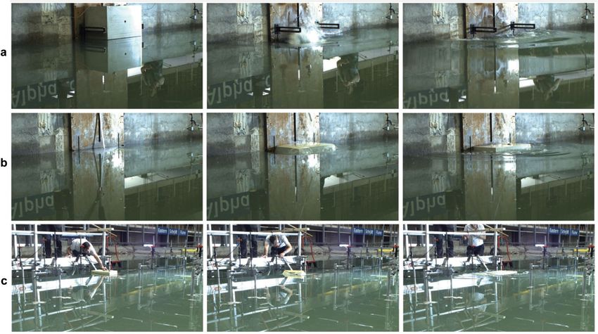
ARTICLE COMMUNICATIONS EARTH & ENVIRONMENT | https://doi.org/10.1038/s43247-021-00179-7
G
lacier calving into the ocean (Fig. 1) is predicted to be one realistic calving front geometries. Although this model success-
of the largest contributions to sea-level rise in the fully couples slow glacier flow with a damage-based calving cri-
future1–3. This process corresponds to ~50% of the mass terion, it cannot simulate tsunamis induced by calving.
loss from ice sheets in Greenland and Antarctica4,5. Glacier cal- Tsunamis generated by landslides were extensively studied24,25.
ving is caused by first, second, and third-order processes. First- Yet, only a few studies focused on tsunamis induced by calving
order processes correspond to the formation of surface crevasses glaciers. Lüthi and Vieli10 reported a 45–50 m tsunami generated
in the ice owing to spatial variation in flow velocity. Second and by the calving of a 200 m high ice cliff of the calving front of the
third-order processes include crack propagation owing to local Eqip Sermia glacier in Greenland. The wave was still 3.3 m large
stress concentrations, ice stretching in the vicinity of the ice front, 4.5 km from the calving outlet and led to a 20 m run-up on the
and oceanic erosion and torque induced by buoyant forces6,7. opposite shore. Recently, Heller et al.13 performed large-scale
Depending on the shape of the glacier outlet, this may lead to laboratory experiments to study the characteristics of waves
different calving scenarios8. Glacier calving can have dramatic generated by different calving mechanisms. These authors
consequences, as falling or capsizing icebergs can generate large showed that empirical equations established for landslides-
tsunamis, which are a threat to coastal infrastructure, ecology, induced tsunamis25 overestimated wave amplitudes and gen-
and people9–15. In high mountain proglacial lakes, calving- erally fail to reproduce the physics of calving-induced tsunamis.
induced waves may further pose major hazards through trigger- Recently, Chen et al.26 were able to reproduce the characteristics
ing lake outburst floods with high destructive potential in of waves reported in Heller et al.13 using foam-extend and the
downstream valleys16. Immersed Boundary Method. Yet, an approach to simulate
Most existing numerical approaches for marine-terminating fracture processes during dynamic glacier calving and tsunamis in
glaciers were developed to study the slow creep of ice using a unified manner is still missing.
continuum Eulerian methods (e.g., Elmer/Ice17), and the calving Here, we report coupled glacier calving and tsunami experi-
rate is generally evaluated using simplified and empirically based ments and develop a continuum damage Material Point Method
calving laws or simple analytic models18. In general, the valida- (MPM) to explicitly simulate ice fracture and hydraulic interac-
tion of these models against observations remains relatively tions. This new model accurately reproduces dynamic ice frac-
limited19 and mostly excludes temporal scales of single calving tures and generated tsunami characteristics for different calving
events. Åström et al.5,20 and Bassis and Jacobs21 developed purely mechanisms for laboratory and real-world scales.
Lagrangian particle-based models, based on a discrete version of
Newton’s equations of motion, to study the dynamics of sea ice Results
and glacier calving. Despite several approximations, including a Ice and water mechanics. To model the dynamic fracture of the
simplified water–ice interaction law, their simulations were able glacier ice, we developed a non-associative elastoplastic model
to reproduce the fractal nature of the debris size distribution20 based on the Cohesive Cam Clay (CCC) yield surface used by
and diverse calving features based on glacier geometry21. How- Gaume et al.27 to simulate snow and avalanche mechanics. A
ever, the discrete nature of these models makes them computa- mixed-mode yield surface such as this was shown to adequately
tionally very expensive and therefore limited to single events. model brittle ice fracture based on experimental data28. However,
Furthermore, the water in their simulation is not explicitly the previously chosen associative flow rule was only adequate
modeled, which prevents the study of the tsunamigenic potential owing to the porous nature of snow, allowing for volume change
of glacier calving. More recently, Mercenier et al.22,23 developed a (compaction hardening). Conversely, in the case of a significantly
transient multiphysics finite element model to simulate the effect less-porous material such as ice, choosing a non-associative flow
of oceanic melt on ice break-off at the terminus of a marine rule29 is key owing to its natural volume-preserving qualities30.
glacier. They showed that a von Mises stress criterion led to As such, we adopt a non-associative flow rule31 coupled with a
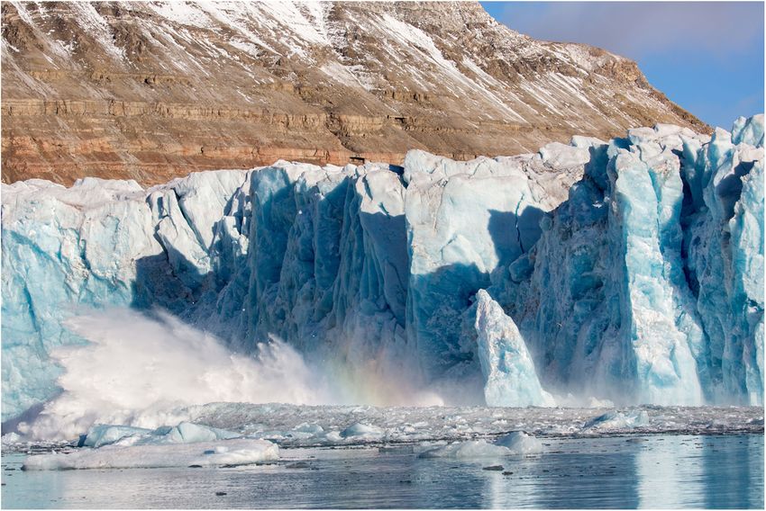
Fig. 1 Calving event triggering a large tsunami. Kongsfjorden, Svalbard. [MB Photography]/[Moment] via Getty Images.
2 COMMUNICATIONS EARTH & ENVIRONMENT | (2021)2:130 | https://doi.org/10.1038/s43247-021-00179-7 | www.nature.com/commsenv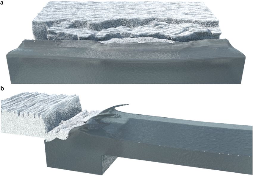
COMMUNICATIONS EARTH & ENVIRONMENT | https://doi.org/10.1038/s43247-021-00179-7 ARTICLE
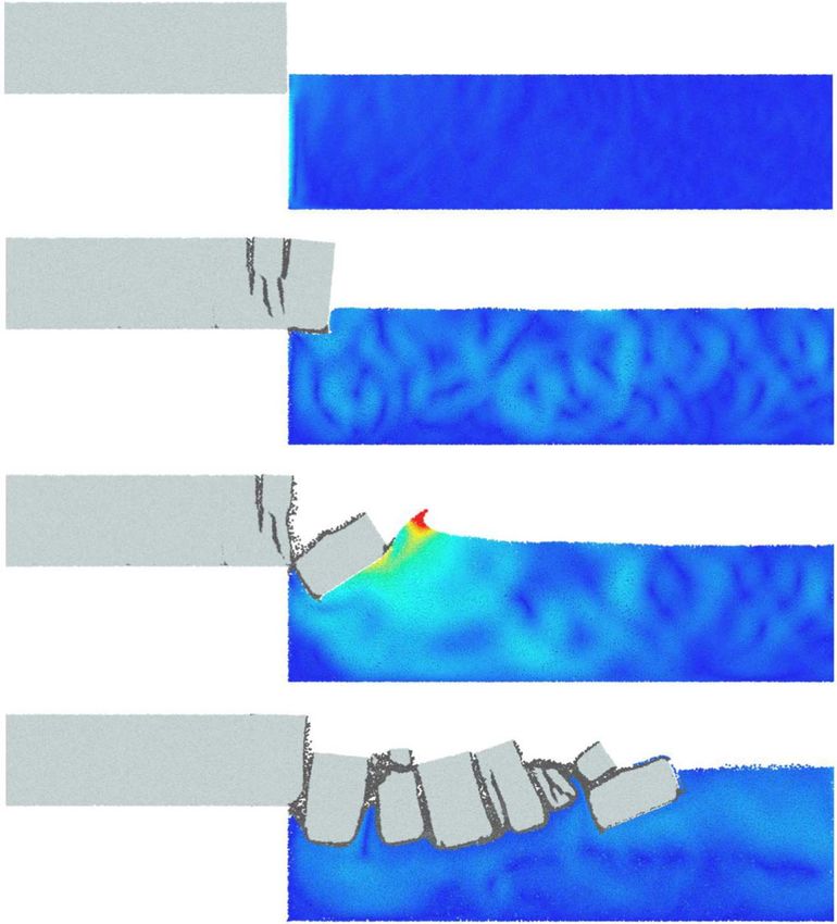
Fig. 2 Comparison between simulations and experiments of tsunamis generated by different calving mechanisms. a MPM simulations of a gravity-
dominated fall of an iceberg (GF, top), buoyancy-dominated fall (BF, middle), and capsizing (CS, bottom) calving mechanisms. The color represents the
velocity of water particles (blue = 0 m/s; red = 0.6 m/s). Movies of these three simulations can be found in the Supplement (Supplementary Movie 1).
b (top) Amplitude of the first generated wave normalized by the maximum wave amplitude as a function of time. The inset shows the modeled maximum
wave amplitude against the observed one from the laboratory experiments of Heller et al.13, including error bars corresponding to uncertainties in the 2D/
3D transformation (see Methods). Time was shifted so that the time corresponding to the maximum wave height corresponds to t = 0 s in all simulations
and experiments.
pffiffiffiffiffiffiffiffi (Bottom) Position of the first generated wave as a function of time. The theoretical prediction for linear shallow-water waves is given by
xth ¼ gDw t.
softening law to model the dynamic ice fracture. The mechanical water tank at varying submergence depth D to modify the
behavior of water is simulated using a nearly incompressible buoyancy contribution and thus, ice fracture features. An exam-
equation of state32. The mass and momentum balance equations ple of simulation result for D/Hi = 0.2 is shown in Fig. 3a and
are solved numerically using the MPM27,33 (see Methods for a Supplementary Movie 2. In this case, the main contribution to
complete model description). instability is gravity. Hence, we observe ice fractures starting to
form at a certain length behind the front, and that propagate from
Calving mechanism and tsunami wave characteristics. In a first the top of the glacier owing to gravity-induced bending. Once
set of experiments, we model the tsunami wave response to three released, the iceberg generates a tsunami that propagates to the
main calving mechanisms according to the laboratory experi- other side of the water tank (see Supplementary Movie 2). If the
ments of Heller et al.13: (i) gravity-dominated fall (GF), (ii) simulation is run for a long time, we observe subsequent
buoyancy-dominated fall (BF), and (iii) capsizing (CS). The detachments of icebergs of similar sizes, hence this length mea-
numerical setup consists of the interaction between a rigid block sure seems a robust output quantity of the model. The first ice-
of density similar to that of ice (920 kg/m3) and a Dw = 1 m deep berg length Li is computed and plotted in Fig. 3b as a function of
water tank (see Methods) in two dimensions. For all simulated the submergence depth—ice height ratio D/Hi. The iceberg length
cases (Fig. 2 and Supplementary Movie 1), a rapid increase of the first increases as submergence depth increases owing to a pro-
wave amplitude is reported until it reaches a maximum value. gressive stabilizing effect of buoyancy. For D/Hi ~ 0.92 = ρi/ρw, no
Then, the wave amplitude significantly decreases. A 2D/3D ice failure is reported as the bending force due to the ice weight is
amplitude transformation factor based on an extensive amount of compensated by the effect of buoyancy. For D/Hi > 0.92, we
experimental data34 (see Methods) was used to compare our observe ice fractures starting from the bottom of the ice slab
results to those of Heller et al.13. A good agreement between our related to the effect of buoyant forces which overcome body
numerical solution and experimental data is observed. In parti- weight forces. In turn, the iceberg length decreases with
cular, the maximum wave amplitude is correctly reproduced in increasing D/Hi. Additional simulation results are shown in the
both capsizing and gravity fall cases and slightly overestimated in Supplement for D/Hi = 0.7 and for lower ice strength values.
the buoyant fall case (Fig. 2b). Concerning the wave velocity, our Numerical results were then compared to a simple analytical
simulation results perfectly follow the ptheoretical limit prediction model which compares the bending stress induced by the inter-
ffiffiffiffiffiffiffiffi play between buoyancy and gravity and the ice tensile strength.
for linear shallow-water waves vw ¼ gDw ; furthermore, a fair
This model (see Methods) leads to the following analytical
agreement with experimental data is reported. Consistent with
expression for the iceberg length:
laboratory experiments, our model results also suggest that
gravity fall cases are the most hazardous as they induce the largest !12
tsunami amplitudes. Li 2σ t 1
¼ ; ð1Þ
Hi 3ρi gH i j1 ρρw HD j
i i
Iceberg sizes: interplay between buoyancy and ice weight. To
evaluate the capabilities of our new constitutive model for ice, we where σt is the tensile strength of ice. Our MPM simulation
perform glacier calving MPM simulations using a simple geo- results are in line with the predictions of this theoretical bending
metry for which analytical solutions exist for validation: an ice model (Fig. 3b) and are consistent with the position of the
block of height Hi is sliding at a constant velocity and enters a modeled stress maxima by Mercenier et al.22.
COMMUNICATIONS EARTH & ENVIRONMENT | (2021)2:130 | https://doi.org/10.1038/s43247-021-00179-7 | www.nature.com/commsenv 3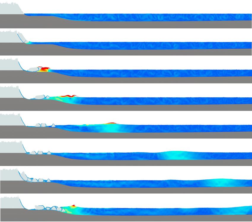
ARTICLE                                                  COMMUNICATIONS EARTH & ENVIRONMENT | https://doi.org/10.1038/s43247-021-00179-7

Fig. 3 Simulations of glacier calving and comparison with an analytical model for the iceberg length. a MPM simulations of glacier calving for Hi = 200
m and D/Hi = 0.2. A movie of this simulation can be found in the Supplement (Supplementary Movie 2). b Iceberg length to height ratio Li/Hi as a function
of the submergence depth to ice height ratio D/Hi. The analytical expression is given by Eq. (1). The water is colored by velocity: blue and red indicate water
moving at 0 m/s and 20 m/s, respectively. The gray color in the glacier represents failed particles.

Calving-induced tsunami at the Eqip Sermia glacier. Given the                    of 32 m/s; furthermore, this agrees with theoretical predictions for
ability of our model to quantitatively reproduce wave and ice                    a fjord water depth estimated between 100 and 150 m36, leading
fracture characteristics, we simulate one past calving event of the              to a theoretical shallow-water velocity range between 31 and
Eqip Sermia, a tidewater outlet glacier in Greenland, for which                  38 m/s.
numerous observations and field measurements are available for
both the glacier and tsunamis10. The geometry of the glacier front
has been initialized according to the real shape of the glacier10.               Discussion
The undulating “crevassed” surface structure has been produced                   We proposed a new model based on the MPM, a hybrid Eulerian-
according to a Simplex Improved Perlin noise35 to mimic the                      Lagrangian numerical technique, to simulate glacier calving and
crevasse distribution of the glacier (Fig. 4 and Supplementary                   tsunami generation. Our nearly incompressible water model was
Movies 3 and 4). The detailed description of this event, the                     able to reproduce well the effects of different iceberg calving
numerical setup, and the parameter calibration are given in the                  mechanisms on the amplitude and speed of the generated tsunamis
Methods. The failed portion of the glacier has a width of 75 m in                measured in laboratory experiments13. Deviations in maximum
our simulations which is slightly larger than the reported value                 wave amplitude can be attributed to the empirical nature of the 2D/
measured between 50 and 60 m. The angle of the failure plane in                  3D transformation (±50% deviation reported in Heller and
our simulation is 54°, in good agreement with the measurements                   Spinneken34). In addition, slight wave velocity deviations from the
(between 45 and 60°). Note that the size of the initial iceberg is               linear shallow-water limit theory can be attributed to the inter-
not only dependent on the relative water level, but also on the                  mediate character and non-linearity of the waves as well as fre-
crevasse distribution, as shown in Fig. 4 where the failure is                   quency dispersion for which variations around the linear wave
initiated at the location of the first deeper crevasse.                           theory expression can reach around ±10% for aw/Dw > 0.0337. This
   The wave amplitude measured in our MPM simulation (Fig. 4)                    wave velocity difference may contribute to the faster amplitude
250 m from the calving front is 50 m, which is in good agreement                 decrease in the gravity-dominated fall and capsizing cases. Our
with the wave amplitude observed at this location (between 45                    model is intended to simulate the complex multiphase interplay
and 50 m)10. A wave amplitude of 3.3 m was measured at the tide                  between ice and water mechanics during glacier calving. Although
gauge on the shore opposite of the glacier. In our 2D simulation,                our water model has been extensively used in Smoothed Particle
the wave amplitude decreases from ~40 to 30 m at a distance of                   Hydrodynamics (SPH) free surface flow simulations of water and
~2000 m from the calving front and then slowly decreases further.                has been validated for several applications32,38–40, solving incom-
We measure a wave amplitude of 27 m at the distance of the tide                  pressible Navier–Stokes equations using computational fluid
gauge, which corresponds to a wave amplitude between 2.5 and                     dynamics would lead to more accurate results for the water
6.6 m in 3D (see Methods) also in good agreement with the                        dynamics41. Yet, it would also computationally be significantly
reported field measurement. Finally, we measure an average wave                   more expensive and challenging to implement within the current
speed of 35 m/s, which also agrees well with the measured value                  hybrid solid-fluid numerical framework.

4             COMMUNICATIONS EARTH & ENVIRONMENT | (2021)2:130 | https://doi.org/10.1038/s43247-021-00179-7 | www.nature.com/commsenv
COMMUNICATIONS EARTH & ENVIRONMENT | https://doi.org/10.1038/s43247-021-00179-7                                                         ARTICLE

Fig. 4 MPM simulation of the Eqip Sermia glacier calving and tsunami generation and propagation. The water is colored by velocity: blue and red
indicate water moving at 0 m/s and 20 m/s, respectively. The blue color in the glacier represents particles for which the yield criterion was met (plastic
deformation). The ice cliff height is ~200 m and the water depth in the main fjord is ~125 m. Movies of this simulation can be found in the Supplement
(Supplementary Movies 3 and 4).

   Our new ice mechanical model has been validated by simu-                   required to capture fast ice fracture are incompatible with such
lating a simple glacier calving geometry for which the competing              slow, viscous deformations. However, one could easily couple the
effects of the glacier weight and buoyant forces lead to different            present model with a standard continuum glacier flow model17,22.
ice fracture mechanisms and iceberg lengths that agreed well with             In addition, note that an assumption in the formulation of our ice
theoretical predictions. When applying the model to a real-world              plastic flow rule gives rise to an analytical solution that speeds up
outlet glacier, the model quantitatively reproduced the iceberg               simulation (see Supplementary Material and Simo44). This sim-
geometry and dimensions as well as the main characteristics of                plified formulation is based on the hypothesis of a relatively stiff
the generated tsunamis. The simulated iceberg length largely                  material (see Eq. (5) in the Supplement), which is fully appro-
depends on the crevasse distribution and the chosen value of the              priate for ice. An iterative return mapping algorithm would be
ice’s tensile strength. We back-calculated the latter such that the           required for very soft matter (see Gaume et al.27).
model results are in good agreement with the observations. Yet,                  The major advantage of our approach compared with existing
we verified that the obtained value was within a realistic range               methods5,20,22,23 is the ability to simulate, in a unified manner, all
based on extensive laboratory research on ice mechanics28,42.                 of the processes related to fast glacier calving including dynamic
Nevertheless, glacial ice has high variability in its mechanical              ice fracture, tsunami formation, and propagation. In addition, we
properties as well as deep crevasses leading to strong anisotropy,            can apply our method to any type of geometry, including complex
which both have not been accounted for here. In turn, one can                 surface crevasses and boundary conditions. This allows us to
expect smaller iceberg size distributions in reality43 (see Supple-           analyze one or multiple subsequent calving events that can be
mentary Figs. 2 and 3). It is important to note that our model                measured, which is crucial for model validation. This unified and
only applies to short time scales for which the ice behaves as a              multiphysics approach prevents us from using model chains5,8,
brittle material. We do not simulate viscous creep, nor the                   which suffer from error propagation. Furthermore, the hybrid
complex basal processes leading to crevasse formation. We could               Eulerian-Lagrangian continuum framework leads to a tre-
implement an ice creep law in our model, but the time-steps                   mendous reduction in the computational time compared with the

COMMUNICATIONS EARTH & ENVIRONMENT | (2021)2:130 | https://doi.org/10.1038/s43247-021-00179-7 | www.nature.com/commsenv                                 5
ARTICLE COMMUNICATIONS EARTH & ENVIRONMENT | https://doi.org/10.1038/s43247-021-00179-7
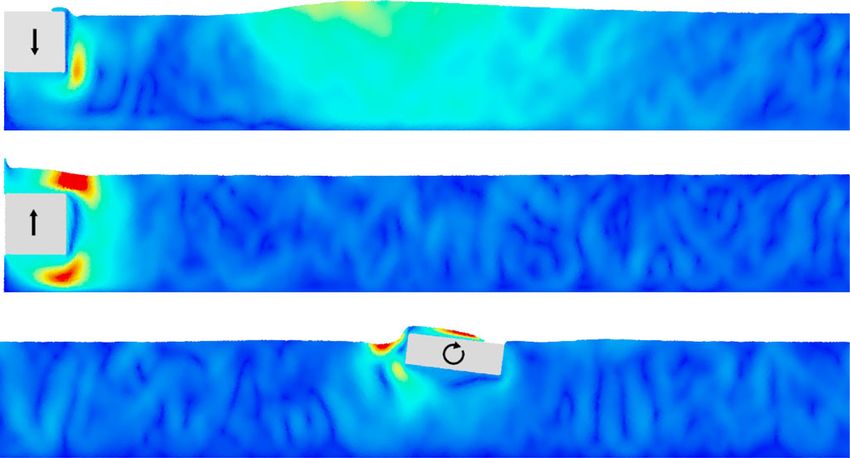
Fig. 5 Three-dimensional simulations of glacier calving and tsunami wave generation. a We simulate a wide glacier to focus on the 3D ice fracture
characteristics. The ice cliff height is 150 m, the water depth is 200 m. The width of the system is 2 km, the glacier length is 1 km and the length of the
water tank is 625 m. This simulation is composed of 36 million particles. A movie of this simulation can be found in the Supplement (Supplementary
Movie 5). b Here, a long water tank is used to focus on the 3D tsunami propagation. The ice cliff height is 200 m and the water depth in the main fjord is
125 m. The width of the system is 400 m and the water tank is 1.6 km long. This simulation is composed of 20 million particles. A movie of this simulation
can be found in the Supplement (Supplementary Movie 6).
discrete element method used in Astrom et al.5. For instance, 3D penalization of shearing and volume change and is written as:
simulations (Fig. 5 and Supplementary Movies 5 and 6) of a single
1 μ κ J2 1
ΨðFÞ ¼ Ψμ ðJ d FÞ þ Ψκ ðFÞ so that Ψμ ðFÞ ¼ ð tr ðFT FÞ dÞ and Ψκ ðJÞ ¼ log ðJÞ
glacier calving event with 20–36 million particles takes 0. Recent triaxial loading laboratory experiments showed that the yield surface
associative elastoplastic model based on the aforementioned CCC yield surface of ice has an elliptical shape in the p−q space50. As a consequence, we chose the
used by Gaume et al.27. This yield surface showed great success for modeling the following CCC yield surface similar to that used for snow by Gaume et al.27 and
plasticity of snow by incorporating its natural cohesive properties; however, the Meschke et al.51:
previously chosen associative flow rule was only adequate owing to the porous yðp; qÞ ¼ q2 ð1 þ 2βÞ þ M 2 ðp þ βp0 Þðp p0 Þ ð5Þ
nature of snow, allowing for some volume change. Conversely, in the case of a
significantly less-porous material such as ice, choosing a non-associative flow rule where β is the cohesion coefficient, M is the slope of the cohesionless critical
is key owing to its natural volume-preserving qualities30. As such, we adopt the state line and p0 is the pre-consolidation pressure. Softening or hardening is
non-associative flow rule proposed by Wolper et al.31 to model the dynamic performed by shrinking or expanding the yield surface through variations in p0
fracture of a variety of solids while ensuring volume preservation. Unfortunately, (Fig. 6). The major difference compared with Gaume et al.27 is in the plastic flow
this approach brings with it a unique problem in the discrete treatment of plas- rule and the hardening variable used for the hardening/softening relationship.
ticity: when stresses are projected to the surface orthogonally to the hydrostatic Snow is a highly porous material, which justified the use of an associative plastic
axis, there is no change in pressure and, as such, no analytic way to compute the flow rule and a hardening law based on the volumetric plastic strain. In contrast,
hardening/softening. Wolper et al. found success in treating this issue using a the failure of ice is not associated with large changes in volume29. Hence, a non-
geometric intersection approach; however, we propose a more physically based associative plastic flow rule has been developed, and a relevant formulation for the
approach that uses quantities we have analytic expressions for. deviatoric plastic strain, α (see definition in Supplementary Note 1 and illustration
First, we outline the elastoplastic theory behind our return mapping approach. in Supplementary Figure 1), is used in the hardening rule as follows:
We use the deformation gradient, F = ∂ϕ/∂X, where ϕ(X, t) denotes a deformation p0 ¼ κ sinhðξ maxðα; 0ÞÞ ð6Þ
map from the undeformed coordinate X to the current configuration x.
Furthermore, we decompose F into an elastic part, FE, and a plastic part, FP, as F = where κ ¼ 23 μ þ λ is the bulk modulus and ξ is the hardening factor. A q-based
FEFP. non-associative projection to the yield surface is performed if the trial elastic
We adopt a split Neo-Hookean hyperelasticity model to predict nonlinear pressure ptr is between −βp0 and p0. If this is not the case, projection is made to the
stress-strain relations suitable to simulating materials undergoing large tips of the yield surface (Fig. 6). The rate of deviatoric plastic deformation is
deformations48; this deviatoric-dilational split energy allows for the separate positive (α_ > 0) if p < pc, leading to material softening; conversely, the rate is
6 COMMUNICATIONS EARTH & ENVIRONMENT | (2021)2:130 | https://doi.org/10.1038/s43247-021-00179-7 | www.nature.com/commsenv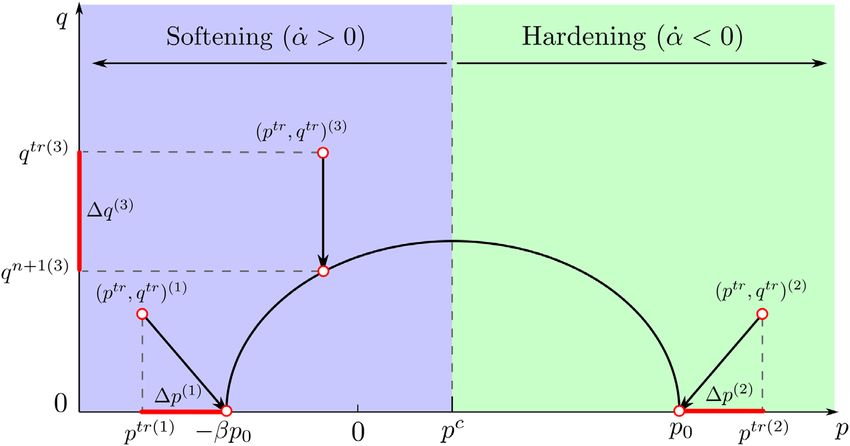
COMMUNICATIONS EARTH & ENVIRONMENT | https://doi.org/10.1038/s43247-021-00179-7                                                                                 ARTICLE

Fig. 6 Cohesive Cam Clay yield surface in the p−q space to illustrate our new q-based hardening approach. Red points represent the p−q state of a
given particle before and after return mapping in each case (see Supplementary Note 1).

negative (α_ < 0) if p > pc, inducing material hardening (see details in
Supplementary Note 1). The proposed deviatoric hardening variable is also                    Table 1 Experimental parameters of the three selected
different from that proposed by Wolper et al.31 who used a non-physically based              laboratory experiments of Heller et al.13.
variable formed from simple geometric considerations.

                                                                                             Block parameters                                          GF       BF        CS
A nearly incompressible fluid model for water. Water is modeled as a nearly
incompressible fluid32 with stress tensor σw and partial stress pw that depends on            Block length (m)                                          0.5      0.5       0.8
the current water density, ρ, and initial water density, ρw, according to:                   Block thickness s (m)                                     0.5      0.5       0.25
                                                                                         Block width b (m)                                         0.8      0.8       0.5
                                                      θ
                      σ w ¼ pw 1; pw ¼ κw ρρ  1                              ð7Þ           Block volume Vs (m3)                                      0.2      0.2       0.1
                                                        w
                                                                                             Block density ρs (kg/m3)                                  936      923       924
where κw is the water bulk modulus and θ is a parameter that penalizes deviations            Block mass ms (kg)                                        187.1    184.6     92.4
from incompressibility. This relationship, which is classically used in water                Water depth Dw (m)                                        1        1         1
simulations using SPH, another particle-based method32, is designed to stiffly                Release position of block base from the still             0.00     −0.83     −0.74
prevent volume change of the water phase.
                                                                                             water surface (m)
                                                                                             Block velocity vs (m)                                     1.15     0.48      0.61
Material Point Method. MPM discretizes a continuum into Lagrangian material                  Froude number F                                           0.37     0.15      0.19
points to track mass, momentum, and deformation gradient, and uses a back-
                                                                                             Relative block thickness S                                0.5      0.5       0.25
ground Eulerian grid to solve mass and momentum conservation as follows:
                                                                                             Relative block mass M                                     0.23     0.23      0.18
                       Dρ                          Dv
                          þ ρ∇  v ¼ 0;        ρ      ¼ ∇  σ þ ρg                   ð8Þ
                       Dt                          Dt
where ρ is density, t is time, v is velocity vector, σ is the Cauchy stress tensor, and g   Experimental data
is the gravitational acceleration vector. In MPM, mass is automatically conserved as        2D/3D transformation. The general expression for the transformation of the 2D to
the mass of each particle is constant. The momentum balance is solved on the                3D primary wave amplitudes is given by Heller and Spinneken34:
background grid through discretization of its weak form. The explicit MPM
                                                                                                             a3D           r 0:40 0:50 0:50 5=6
algorithm by Stomakhin et al.52 is applied with a symplectic Euler time integrator.                               ¼ 1:5       F    S     M              fγ              ð11Þ
Details of the adopted MPM time-stepping algorithm can be found in27,52,53. In                               a2D          Dw
contrast with Gaume et al.27, we use the Affine Particle-In-Cell (APIC) method54 to          where r is the radial distance from the impact, Dw is the water depth, γ is the wave
perform MPM transfer operations, which allows for better conservation of both               propagation angle, and the parameters F, S, and M are the slide Froude number, the
linear and angular momentum.                                                                relative slide thickness, and the relative slide mass, respectively, and defined as
    The Cauchy stress tensor σ in Eq. (8) is related to the strain as follows               follows:
                                             1 ∂Ψ T                                                                       vs             s            ms
                                       σ¼         F                                  ð9Þ                          F ¼ pffiffiffiffiffiffiffiffi ; S¼       ; M¼             ;                ð12Þ
                                             J ∂FE E                                                                      gDw          Dw           ρw bD2w

where Ψ is the elastoplastic potential energy density, FE is the elastic part of the        where vs is the slide velocity, s is the slide thickness, ms is the slide mass, and b is
deformation gradient, F, and J ¼ detðFÞ.                                                    the slide width. The function fγ is defined as
                                                                                                                       f γ ¼ cos2ð1þexp½0:2ðr=Dw ÞÞ ð2γ=3Þ                 ð13Þ
Iceberg length theoretical model. Our choice to simulate glacier calving on a               Iceberg-tsunami laboratory experiments. We conducted the experiments in the
simple geometry is motivated by the existence of a simplified analytical solution for        Delta Basin of Deltares, Delft, with effective size, excluding wavemakers and
model validation. This solution has been derived based on the bending stresses              absorbing beaches, of 40.3 m × 33.9 m. The total number of experiments was 66.
induced by gravitational forces (from the interplay between the ice weight and              The following provides an overview of the three herein selected experiments with
buoyancy) using beam theory55. Ice fracture requires that the total bending stress          further details for all experiments given by Heller et al.13,37.
induced by this interplay exceeds the ice’s tensile strength, σt. Bending stresses can          Table 1 shows the relevant parameters. We modeled the icebergs with
be computed according to σ = Mz/I where M is the bending moment, z is the                   polypropylene homopolymer blocks with a density similar to that of ice. The
vertical coordinate (above the neutral surface), and I is the moment of inertia. This       0.500 m × 0.800 m × 0.500 m block in the gravity- and buoyancy-dominated fall
leads to the following instability criterion:                                               cases was released at the vertical boundary of the basin and the 0.500 m ×
                                                                                          0.800 m × 0.250 m block in the capsizing case was released offshore. The blocks
                              3ρ gL2 3ρ gL2
                              i i                                                         weighed up to 187.1 kg and the still water depth was 1.00 m.
                                        w i  ¼ σt
                              2H i          2D
                                          |fflfflffl{zfflfflffl}                              ð10Þ          Three types of experiments were conducted: (i) GF, (ii) BF, and (iii) CS. For GF
                               |fflffl{zfflffl}
                                ice weight   buoyancy                                       cases, we held the block in position with an electromagnet prior to release, which
                                                                                            was connected to a rope. We fixed the supporting frame for this electromagnet and
which leads to Eq. (1).                                                                     the block to a steel plate at the basin wall. The block was moved in the vertical

COMMUNICATIONS EARTH & ENVIRONMENT | (2021)2:130 | https://doi.org/10.1038/s43247-021-00179-7 | www.nature.com/commsenv                                                           7
ARTICLE COMMUNICATIONS EARTH & ENVIRONMENT | https://doi.org/10.1038/s43247-021-00179-7
Fig. 7 Pictures of the laboratory experiments. a Gravity-dominated fall; b Buoyancy-dominated fall; c capsizing. From Heller et al.13.
Table 2 Numerical and mechanical parameters used in the simulations.
Case Δx (m) Np ρi (kg/m3) Ei (GPa) νi ρw (kg/m3) Water model (κ (MPa), θ) NACC (βp0 (MPa), ξ, M)
Tsunami laboratory (Fig. 2) 0.01 640 k 920 - - 1000 (10, 7) -
Simple geometry (Fig. 3) Hi/40 55 k–79 k 900 1 0.3 1000 (10, 7) (0.5, 3, 1.4)
Tsunami Eqip Sermia (Fig. 4) 2.5 370 k 900 1 0.3 1000 (10, 7) (0.8, 0.1, 0.13)
3D calving 1 (Fig. 5a) 5 36 M 900 10 0.3 1000 (10, 7) (2, 3, 1.4)
3D calving 2 (Fig. 5b) 5 20 M 900 0.1 0.3 1000 (10, 7) (0.5, 3, 1.4)
direction towards the release position using a winch system fixed to a support boat was registered with the TRI, such that the tsunami wave height from the
structure outside the basin. For BF cases, the block was pulled underwater to the videos could be geometrically determined. The wave height in the impact zone on
release position with a rope attached to the center of the block base. We further the shore opposite of the glacier was registered with a pressure sensor at a 4 s
stabilized the block with a steel beam from above (Fig. 7) and released both the interval.
beam and the rope simultaneously to initiate waves. Concerning the 2D/3D transformation, the following ranges of F, S, and M have
For CS cases, we held the block in position with a wooden rod guided through been used10 in the article:
the center of the block. Steel profiles on both sides accommodated this rod such
that the block was able to heave and pitch, but not to sway and surge. We initiated F GF ¼ 2:1 3 ; SGF ¼ 1:5 2:5 ; M GF ¼ 5 20 ð14Þ
capsizing by removing a fitting that stabilized the block and then simply releasing
the block by hand (Fig. 7). Setup of the simulations. In all our simulations, the resolution of the MPM
The velocity vs corresponds to the fastest moving section of the block derived background mesh was chosen 40–50 times smaller than the minimum character-
from the recordings of a nine Degree of Freedom motion sensor (Adafruit istic geometrical length of the system (rigid block length, glacier height, or water
BNO055) with a procedure described in Chen et al.26. The sensor was located in a depth). In 2D and 3D simulations, we used approximately four and eight material
watertight enclosure and attached to the block surface. We extracted the still points per element, respectively. In addition, the time step was evaluated based on
images shown in Fig. 7 from camera footage recorded with a 5 MP PointGrey both the CFL and elastic wave speeds to ensure the stability of the simulation.
ZBR2-PGEHD-50S5C-CS camera at 15 Hz. We used up to 35 resistance-type wave
probes to record the wave features. Relative to the coordinate origins at the front of Tsunami (Fig. 2). A 2D water tank of 16 m × 1 m is simulated. For GF and BF
the steel plate in the center of the block in the cross-shore direction (GF and BF simulations, a solid block of 0.5 m × 0.5 m is used. In the GF experiment, the block
cases) and at the block center (CS case), we arranged these probes at different is released on the left side of the tank with the bottom at the level of the water’s free
points in the range of relative radial distances r/Dw = 2–35 and wave propagation surface. For the BF case, the block is released with the bottom at a depth of −0.83
angles γ = 0∘ (block axis) to −75∘ (fall cases) and r/Dw = 2–15 and γ = 0∘ to −180∘ m corresponding to the experimental setup (Table 1). For the CS simulation, a solid
(capsizing case). The angle γ is thereby defined positively in the clockwise direction. block of 0.8 m × 0.25 m is used and released from a neutrally floating position with
We shortened the water surface time series individually to remove data affected by an initial angle of 35° to activate capsizing in a similar way as in the experiments
reflection from the basin boundaries and filtered most wave probe data with a low- (small initial movement by hand). For all cases, we use a block density of 920 kg/m3
pass filter with a cutoff frequency at 9–11 Hz37. (similar to that of ice). The numerical and mechanical parameters are presented in
Table 2.
Eqip Sermia glacier calving—tsunami field experiments. Glacier calving activity at
Eqip Sermia was investigated with a terrestrial radar interferometer (TRI), surveys Effect of buoyancy on iceberg lengths (Fig. 3). A 2D water tank of length 250 × N m
with unmanned aerial vehicles (drones), pressure sensors, and time-lapse and depth 50 × N + Dw m is simulated with N ∈ {1, 3, 5, 10}. The ice slab has a
cameras56. The ice wall collapse and the ensuing tsunami were filmed by tourists length of 150 × N m and a cliff height of Hi = N × 40pm.
ffiffiffiffi The ice slab slides on a
on a tour boat. The exact thickness of removed ice was determined at high spatial frictionless boundary condition with a speed of 1 ´ N m/s. Simulations are per-
resolution (10 m pixel size) from TRI interferograms, as was the terminus geometry formed with a constant water level, i.e., the water level increase due to iceberg
before, during and after the collapse (Lüthi and Vieli10). The position of the tour generation is compensated by water particles exiting the water tent at the water
8 COMMUNICATIONS EARTH & ENVIRONMENT | (2021)2:130 | https://doi.org/10.1038/s43247-021-00179-7 | www.nature.com/commsenvCOMMUNICATIONS EARTH & ENVIRONMENT | https://doi.org/10.1038/s43247-021-00179-7 ARTICLE
tank outlet. The water tank has frictionless walls. The numerical and mechanical 7. Benn, D. I. et al. Melt-under-cutting and buoyancy-driven calving from
parameters are presented in Table 2. In this case, generic mechanical properties tidewater glaciers: new insights from discrete element and continuum model
falling within a realistic range of reported values for ice28 were chosen for the sake simulations. J. Glaciol. 63, 691–702 (2017).
of the comparison with the analytical model. An elastic modulus of 1 GPa was 8. Benn, D. I. & Aström, J. A. Calving glaciers and ice shelves. Adv. Phys 3,
chosen following Astrom et al.5,20. 1513819 (2018).
9. Reeh, N. Long calving waves. In POAC’85, 8th International Conference on
Calving-induced tsunami at the Eqip Sermia glacier (Fig. 4). We simulated a 2D Port and Ocean Engineering Under Arctic Conditions (1985).
water tank of length 4500 m with variable depth. The first 500 m of the fjord have an 10. Lüthi, M. P. & Vieli, A. Multi-method observation and analysis of a tsunami
average depth of 35 m and smoothly increases to a depth of ~135 m in the main fjord, caused by glacier calving. Cryosphere 10, 995–1002 (2016).
in agreement with field observations10. The ice cliff is 200 m high and the real-world 11. MacAyeal, D. R., Abbot, D. S. & Sergienko, O. V. Iceberg-capsize
shape of the calving ice mass measured in Lüthi and Vieli36 has been modeled. The tsunamigenesis. Ann. Glaciol. 52, 51–56 (2011).
crevasse distribution has been simulated according to the Perlin simplex terrain noise 12. Levermann, A. When glacial giants roll over. Nature 472, 43–44 (2011).
model35 leading to surface crevasses typically between 20 and 50 m deep and crack 13. Heller, V. et al. Large-scale experiments into the tsunamigenic potential of
openings between 5 and 10 m. Parameters are presented in Table 2. In this case, different iceberg calving mechanisms. Sci. Rep. 9, 1–10 (2019).
model parameters were back-calculated within a range of realistic values for ice28,42 to 14. Mikkelsen, N. & Ingerslev, T.Nomination of the Ilulissat Icefjord for inclusion
achieve good agreement (iceberg size and failure angle) with observations. An elastic in the World Heritage List (Geological Survey of Denmark and Greenland,
modulus of 1 GPa was chosen following Astrom et al.5,20. 2003).
15. Huge iceberg threatens tiny Greenland village. The Guardian (2018). Https://
3D glacier calving (Fig. 5a). We simulated a glacier that is 1 km long, 2 km wide and www.theguardian.com/world/2018/jul/14/huge-iceberg-threatens-village-in-
has a 150 m irregular vertical cliff. The water tank is 200 m deep. The submergence greenland.
depth is 40 m corresponding to Hi/D ~ 0.26. The glacier is supported by a fric- 16. Clague, J. J. & O’Connor, J. E. Glacier-related outburst floods. In Snow and ice-
tionless base that slides backward at a speed of 3 m/s, in order to progressively related hazards, risks and disasters (Elsevier, 2020).
remove basal support at the calving front and thus induce calving. Initial cracks 17. Gagliardini, O. et al. Capabilities and performance of elmer/ice, a new-
have been placed within the glacier to mimic crevasses. These initial cracks follow a generation ice sheet model. Geosci. Model Dev. 6, 1299–1318 (2013).
Voronoi distribution with cell size r = (30, 80, 160) m. Parameters are presented in 18. Bassis, J. & Walker, C. Upper and lower limits on the stability of calving
Table 2. Generic yield surface parameters were chosen in agreement with experi- glaciers from the yield strength envelope of ice. Proc. R. Soc. A 468, 913–931
mental data28. Concerning the elastic modulus, most studies related to glacier (2012).
calving numerical simulations use elastic moduli for ice lower than experimentally 19. Amaral, T., Bartholomaus, T. & Enderlin, E. Evaluation of iceberg calving
measured values to speed up simulation5,20 (as the time step depends on the elastic models against observations from Greenland outlet glaciers. J. Geophys. Res.
wave speed). In this simulation, to test the capabilities of our model in simulating Earth Surf. 125, e2019JF005444 (2019).
large-scale calving events with realistic properties, we used an elastic modulus of 20. Aström, J. et al. A particle based simulation model for glacier dynamics.
E = 10 GPa based on experimentally measured values42.
Cryosphere 7, 1591-1602 (2013).
21. Bassis, J. N. & Jacobs, S. Diverse calving patterns linked to glacier geometry.
3D glacier calving and tsunami generation (Fig. 5b). We simulated a water tank of Nat. Geosci. 6, 833–836 (2013).
variable depth: the first 500 m are 300 m deep, and then the next 1250 m are 135 m 22. Mercenier, R., Lüthi, M. P. & Vieli, A. A transient coupled ice flow-damage
deep. The ice slab is 600 m long and has a 200 m irregular vertical cliff. The model to simulate iceberg calving from tidewater outlet glaciers. J. Adv. Model.
crevasse distribution is the same as in the Eqip Sermia 2D simulation. The sub- Earth Syst. 11, 3057–3072 (2019).
mergence depth is 50 m corresponding to Hi/D ~ 0.2. The glacier slides over a 23. Mercenier, R., Lüthi, M. & Vieli, A. How oceanic melt controls tidewater
frictionless boundary condition at a speed of 3 m/s. Parameters are presented in glacier evolution. Geophys. Res. Lett. 47, 2019GL086769 (2020).
Table 2. In this case, a low elastic modulus value was chosen to speed up the
24. Heller, V., Hager, W. H. & Minor, H.-E. Landslide generated impulse waves in
simulation (which suffers from the large size of the water tank). Generic values of
reservoirs: basics and computation. VAW-Mitteilungen 211 (2009).
the yield surface parameters were chosen within a realistic range28,42. An elastic
25. Evers, F., Heller, V., Fuchs, H., Hager, W. H. & Boes, R. Landslide-generated
modulus of 0.1 GPa was chosen following Astrom et al.20 to speed up this simu-
impulse waves in reservoirs: basics and computation. 2nd edn, VAW-
lation and focus on tsunami characteristics.
Mitteilungen 254 (2019).
26. Chen, F., Heller, V. & Briganti, R. Numerical modelling of tsunamis generated
Data availability by iceberg calving validated with large-scale laboratory experiments. Adv.
The data corresponding to the iceberg-tsunami laboratory experiments can be found at Water Resour. 142, 103647 (2020).
https://hydralab.eu/research--results/ta-projects/project/hydralab-plus/11/. The data 27. Gaume, J., Gast, T., Teran, J., van Herwijnen, A. & Jiang, C. Dynamic
corresponding to the Eqip Sermia glacier calving—tsunami field experiments can be anticrack propagation in snow. Nat. Commun. 9, 3047 (2018).
found in a previous publication at https://tc.copernicus.org/articles/10/995/2016/. 28. Derradji-Aouat, A. Multi-surface failure criterion for saline ice in the brittle
regime. Cold Reg. Sci. Technol. 36, 47–70 (2003).
29. Ringeisen, D., Tremblay, L. B. & Losch, M. Non-normal flow rules affect
Code availability fracture angles in sea ice viscous-plastic rheologies. The Cryosphere
The CD-MPM code is open-access and available on GitHub at the following address:
Discussions 1–24 (2020).
https://github.com/penn-graphics-research/ziran2019.
30. Rist, M. & Murrell, S. Ice triaxial deformation and fracture. J. Glaciol. 40,
305–318 (1994).
Received: 4 September 2020; Accepted: 30 April 2021; 31. Wolper, J. et al. CD-MPM: continuum damage material point methods for
dynamic fracture animation. ACM Trans. Graph. 38, 4 (2019).
32. Becker, M. & Teschner, M. Weakly compressible SPH for free surface
flows. In Proc ACM SIGGRAPH/Eurograph Symp Comp Anim, 209–217
(2007).
33. Sulsky, D., Chen, Z. & Schreyer, H. L. A particle method for history-
References dependent materials. Comp. Methods Appl. M 118, 179–196 (1994).
1. Moore, J. C., Grinsted, A., Zwinger, T. & Jevrejeva, S. Semiempirical 34. Heller, V. & Spinneken, J. On the effect of the water body geometry on
and process-based global sea level projections. Rev. Geophys. 51, 484–522 landslide–tsunamis: physical insight from laboratory tests and 2d to 3d wave
(2013). parameter transformation. Coast. Eng. 104, 113–134 (2015).
2. Catania, G., Stearns, L., Moon, T., Enderlin, E. & Jackson, R. Future evolution 35. Perlin, K. Improving noise. In ACM Transactions on Graphics (TOG), 21,
of Greenland’s marine-terminating outlet glaciers. J. Geophys. Res. Earth Surf. 681–682 (ACM, 2002).
125, e2018JF004873 (2020). 36. Lüthi, M. P. et al. A century of geometry and velocity evolution at Eqip
3. Pattyn, F. & Morlighem, M. The uncertain future of the Antarctic ice sheet. Sermia, West Greenland. J. Glaciol. 62, 640–654 (2016).
Science 367, 1331–1335 (2020). 37. Heller, V., Attili, T., Chen, F., Gabl, R. & Wolters, G. Large-scale investigation
4. Rignot, E., Velicogna, I., van den Broeke, M. R., Monaghan, A. & Lenaerts, J. into iceberg-tsunamis generated by various iceberg calving mechanisms.
T. Acceleration of the contribution of the Greenland and Antarctic ice sheets Coast, Eng. 163, 103745 (2021).
to sea level rise. Geophys. Res. Lett. 38, L05503(2011). 38. Dao, M., Xu, H., Chan, E. & Tkalich, P. Numerical modelling of extreme
5. Aström, J. A. et al. Termini of calving glaciers as self-organized critical waves by smoothed particle hydrodynamics. Nat. Hazards Earth Syst. Sci. 11,
systems. Nat. Geosci. 7, 874 (2014). 419 (2011).
6. Benn, D. I., Warren, C. R. & Mottram, R. H. Calving processes and the 39. Xu, X. An improved SPH approach for simulating 3d dam-break flows with
dynamics of calving glaciers. Earth-Sci. Rev. 82, 143–179 (2007). breaking waves. Comput. Methods Appl. M. 311, 723–742 (2016).
COMMUNICATIONS EARTH & ENVIRONMENT | (2021)2:130 | https://doi.org/10.1038/s43247-021-00179-7 | www.nature.com/commsenv 9ARTICLE COMMUNICATIONS EARTH & ENVIRONMENT | https://doi.org/10.1038/s43247-021-00179-7
40. Shao, J., Yang, Y., Gong, H. & Liu, M. Numerical simulation of water Contract no. 654110. J.W. and C.J. were supported in part by DOE ORNL-4000171342,
entry with improved SPH method. Int. J. Comput. Methods 16, 1846004 NSF CAREER (IIS-1943199), and CCF-1813624.
(2019).
41. Yavari-Ramshe, S. & Ataie-Ashtiani, B. Numerical modeling of subaerial and
submarine landslide-generated tsunami waves-recent advances and future
Author contributions
J.W. developed the non-associative elastoplastic model and wrote the corresponding
challenges. Landslides 13, 1325–1368 (2016).
methods section under the supervision of C.J., J.G., and M.G. The MPM code and the
42. Petrovic, J. J. Review mechanical properties of ice and snow. J. Mater. Sci. 38,
APIC transfer scheme was developed by C.J. The field experiments at the Eqip Sermia
1–6 (2003).
glacier were performed by M.L. and A.V. who provided expertise on glacier calving
43. Gaume, J. et al. Evaluation of slope stability with respect to snowpack spatial
processes. V.H. performed the tsunami laboratory experiments and advised on calving-
variability. J. Geophys. Res. 119, 1783–1789 (2014).
induced tsunamis. J.W., M.G., and J.G. performed the simulations. J.G. obtained the
44. Simo, J. C. A framework for finite strain elastoplasticity based on maximum
collaborating funds, designed the study and wrote the paper with J.W. and essential
plastic dissipation and the multiplicative decomposition: Part i. continuum
inputs from all co-authors.
formulation. Comput. Methods Appl. M. 66, 199–219 (1988).
45. Naaim, M. Impulse water waves generated by snow avalanches. In
International Snow Science Workshop (ISSW), pp–619 (Irstea, ANENA, 2013).
46. Zitti, G., Ancey, C., Postacchini, M. & Brocchini, M. Impulse waves generated Competing interests
by snow avalanches: momentum and energy transfer to a water body. J. The authors declare no competing interests.
Geophys. Res. Earth Surf. 121, 2399–2423 (2016).
47. Zitti, G., Ancey, C., Postacchini, M. & Brocchini, M. Snow avalanches striking
water basins: behaviour of the avalanche’s centre of mass and front. Nat. Additional information
Hazards 88, 1297–1323 (2017). Supplementary information The online version contains supplementary material
48. Yue, Y. et al. Hybrid grains: Adaptive coupling of discrete and continuum available at https://doi.org/10.1038/s43247-021-00179-7.
simulations of granular media. In SIGGRAPH Asia 2018 Technical Papers,
SIGGRAPH Asia ’18, 283:1–283:19 (2018). Correspondence and requests for materials should be addressed to J.G.
49. Schofield, A. & Wroth, P.Critical state soil mechanics (McGraw-Hill, 1968).
50. Zhou, Z. et al. Yield surface evolution for columnar ice. Results Phys. 6, Peer review information Primary handling editor: Joseph Aslin.
851–859 (2016).
51. Meschke, G., Liu, C. & Mang, H. A. Large strain finite-element analysis of Reprints and permission information is available at http://www.nature.com/reprints
snow. J. Eng. Mech. 122, 591–602 (1996).
52. Stomakhin, A., Schroeder, C., Chai, L., Teran, J. & Selle, A. A material Publisher’s note Springer Nature remains neutral with regard to jurisdictional claims in
point method for snow simulation. ACM Trans. Graph. 32, 102:1–102:10 (2013). published maps and institutional affiliations.
53. Jiang, C., Schroeder, C., Teran, J., Stomakhin, A. & Selle, A. The material point
method for simulating continuum materials. In ACM SIGGRAPH 2016
Course, 24:1–24:52 (2016). Open Access This article is licensed under a Creative Commons
54. Jiang, C., Schroeder, C. & Teran, J. An angular momentum conserving affine- Attribution 4.0 International License, which permits use, sharing,
particle-in-cell method. J. Comput. Phys. 338, 137–164 (2017). adaptation, distribution and reproduction in any medium or format, as long as you give
55. Timoshenko, S. & Goodier, J.Theory of Elasticity, 37 (McGraw-Hill, 1970).
appropriate credit to the original author(s) and the source, provide a link to the Creative
56. Walter, A., Lüthi, M. P. & Vieli, A. Calving event size measurements and
Commons license, and indicate if changes were made. The images or other third party
statistics of Eqip Sermia, Greenland, from terrestrial radar interferometry.
material in this article are included in the article’s Creative Commons license, unless
Cryosphere 14, 1051–1066 (2020).
indicated otherwise in a credit line to the material. If material is not included in the
article’s Creative Commons license and your intended use is not permitted by statutory
regulation or exceeds the permitted use, you will need to obtain permission directly from
Acknowledgements the copyright holder. To view a copy of this license, visit http://creativecommons.org/
J.G. acknowledges financial support from the Swiss National Science Foundation (SNF) licenses/by/4.0/.
grant PCEFP2_181227. The field work at Eqip Sermia was supported by SNF grant
200021_156098. The laboratory tests were supported by the European Community’s
© The Author(s) 2021
Horizon2020 Research and Innovation Program through the grant to HYDRALAB+,
10 COMMUNICATIONS EARTH & ENVIRONMENT | (2021)2:130 | https://doi.org/10.1038/s43247-021-00179-7 | www.nature.com/commsenvYou can also read