Meta-Learning Dynamics Forecasting Using Task Inference
←
→
Page content transcription
If your browser does not render page correctly, please read the page content below
Meta-Learning Dynamics Forecasting Using
                                                               Task Inference

                                                               Rui Wang*                                 Robin Walters*
                                                   University of California, San Diego                Northeastern University
                                                          ruw020@ucsd.edu                          rwalters@northeastern.edu
arXiv:2102.10271v3 [cs.LG] 23 Aug 2021

                                                                                      Rose Yu
                                                                         University of California, San Diego
                                                                                roseyu@ucsd.edu

                                                                                      Abstract
                                                  Current deep learning models for dynamics forecasting struggle with generalization.
                                                  They can only forecast in a specific domain and fail when applied to systems
                                                  with different parameters, external forces, or boundary conditions. We propose
                                                  a model-based meta-learning method called DyAd which can generalize across
                                                  heterogeneous domains by partitioning them into different tasks. DyAd has two
                                                  parts: an encoder which infers the time-invariant hidden features of the task with
                                                  weak supervision, and a forecaster which learns the shared dynamics of the entire
                                                  domain. The encoder adapts and controls the forecaster during inference using
                                                  adaptive instance normalization and adaptive padding. Theoretically, we prove
                                                  that the generalization error of such procedure is related to the task relatedness
                                                  in the source domain, as well as the domain differences between source and
                                                  target. Experimentally, we demonstrate that our model outperforms state-of-the-art
                                                  approaches on both turbulent flow and real-world ocean data forecasting tasks.

                                         1   Introduction
                                         Modeling dynamical systems with deep learning has shown great success in a wide range of systems
                                         from fluid mechanics to neural dynamics [54, 9, 21, 65, 26]. However, the main limitation of previous
                                         works is very limited generalizability. Most approaches only focus on a specific system and train
                                         on past data in order to predict the future. Thus a new model must be trained to predict a system
                                         with different dynamics. Consider, for example, learning fluid dynamics; shown in Fig. 1are two
                                         fluid flows with different degrees of turbulence. Even though the flows are governed by the same
                                         equations, the difference in buoyant forces would require two separate deep learning models to
                                         forecast. Therefore, it is imperative to develop generalizable deep learning models for dynamical
                                         systems that can learn and predict well over a large heterogeneous domain.
                                         Meta-learning [53, 8, 11], or learning to learn, improves generalization by learning multiple tasks
                                         from the environment. Recent developments in meta-learning have been successfully applied to
                                         few-shot classification [36], active learning [64], and reinforcement learning [15]. However, meta-
                                         learning in the context of forecasting high-dimensional physical dynamics has not been studied before.
                                         The challenges with meta-learning dynamical systems are unique in that (1) we need to efficiently
                                         infer the latent representation of the dynamical system given observed time series data, (2) we need
                                         to account for changes in unknown initial and boundary conditions, and (3) we need to model the
                                         temporal dynamics across heterogeneous domains.
                                         Our approach is inspired by the fact that similar dynamical systems may share time-invariant hidden
                                         features. Even the slightest change in these features may lead to vastly different phenomena. For

                                         *Equal Contribution.
...

                                                                                     time

                                  ...               ?

Figure 1: Meta-learning dynamic forecasting on turbulent flow. The model needs to generalize to a
flow with a very different buoyant force.

example, in climate science, fluids are governed by a set of differential equations called Navier-
Stokes equations. Some features such as kinematic viscosity and external forces (e.g. gravity), are
time-invariant and determine the flow characteristics. By inferring this latent representation, we can
model diverse system behaviors from smoothly flowing water to atmospheric turbulence.
Inspired by neural style transfer [19], we propose a model-based meta-learning method, called DyAd,
which can rapidly adapt to systems with varying dynamics. DyAd has two parts, an encoder g and
a forecaster f . The encoder maps different dynamical systems to time-invariant hidden features
representing constants of motion, boundary conditions, and external forces which characterize the
system. The forecaster f then takes the hidden representations and the past system states to forecast
the future system state. Controlled by the time-invariant hidden features, the forecaster has the
flexibility to adapt to a wide range of systems with heterogeneous dynamics.
Unlike gradient-based meta-learning techniques such as MAML [11], DyAd automatically adapts
during inference using an encoder and does not require any retraining. Similar to model-based
meta-learning methods such as MetaNets [36], we employ a two-part design with an adaptable learner
which receives task-specific weights. However, for time series forecasting, since input and output
come from the same domain, a support set of labeled data is unnecessary to define the task. The
encoder can infer the task directly from query input.
Our contributions include:

       • A novel model-based meta-learning method (DyAd) for dynamic forecasting in large hetero-
         geneous domains.
       • An encoder capable of extracting the time-invariant hidden features of a dynamical system
         using time-shift invariant model structure and weak supervision.
       • A new adaptive padding layer (AdaPad), designed for adapting to boundary conditions.
       • Theoretical guarantees for DyAd on the generalization error of task inference in the source
         domain as well as domain adaptation to the target domain.
       • Improved generalization performance on heterogeneous domains such as fluid flow and sea
         temperature forecasting, even to new tasks outside the training distribution.

2     Methods
2.1   Meta-learning in dynamics forecasting

Let x ∈ Rd be a d-dimensional state of a dynamical system governed by parameters ψ. The problem
of dynamics forecasting is that given a sequence of past states (xt−l+1 , . . . , xt ), we want to learn a
map f such that:
                            f : (xt−l+1 , . . . , xt ) 7−→ (xt+1 , . . . xt+h ).                       (1)
Here l is the length of the input series, and h is the forecasting horizon in the output.
Existing approaches for dynamics forecasting only predict future data for a specific system as a
single task. Here a task refers to forecasting for a specific system with a given set of parameters. The
resulting models often generalize poorly to different system dynamics. Thus a new model must be
trained to predict for each specific system.

                                                    2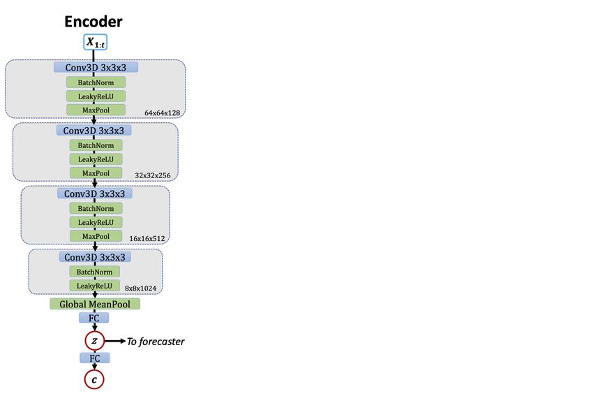
Figure 2: Overview of DyAd applied to two inputs of fluid turbulence, one with small external forcing
and one with larger external forces. The encoder infers the time-shift invariant characteristic variable
z which is used to adapt the forecaster network.

To perform meta-learning, we identify each forecasting task by some parameters c ⊂ ψ, such as
constants of motion, external forces, and boundary conditions. We learn multiple tasks simultaneously
and infer the task from data. Here we use c for a subset of system parameters ψ, because we usually
do not have the full knowledge of the system dynamics. In the turbulent flow example, the state xt is
the velocity field at time t. Parameters c can represent Reynolds number, average vorticity, average
magnitude, or a vector of all three.
Formally, let µ be the data distribution over X × Y representing the function f : X → Y where
X = Rd×l and Y = Rd×h . Our main assumption is that the domain X can be partitioned into
separate tasks X = ∪c∈C Xc , where Xc is the domain for task c and C is the set of all tasks. The data
in the same task share the same set of parameters. Let µc be the conditional distribution over Xc × Y
for task c.
During training, the model is presented with data drawn from a subset of tasks {(x, y) : (x, y) ∼
µc , c ∼ C}. Our goal is to learn the function f : X → Y over the whole domain X which can thus
generalize across all tasks c ∈ C. To do so, we need to learn the map g : X → C taking x ∈ Xc to c
in order to infer the task with minimal supervision.

2.2   DyAd: Dynamic Adaptation Network

We propose a model-based meta-learning approach for dynamics forecasting. Given multiple fore-
casting tasks, we propose to learn the function f in two stages, that is, by first inferring the task c
from the input x, and then adapting to a specialized forecaster fc : Xc → Y for each task.
An alternative is to use a single deep neural network to directly model f in one step over the whole
domain. But this requires the training set to have good and uniform coverage of the different tasks. If
the data distribution µ is highly heterogeneous or the training set is not sampled i.i.d. from the whole
domain, then a single model may struggle with generalization.
We hypothesize that by partitioning the domain into different tasks, the model would learn to pick
up task-specific features without requiring uniform coverage of the training data. Furthermore, by
separating task inference and forecasting into two stages, we allow the forecaster to rapidly adapt to
new tasks that never appeared in the training set.
As shown in Fig. 2, our model consists of two parts: an encoder g and a forecaster f . We introduce
zc as a time-invariant hidden feature for task c. We assume that c depends linearly on the hidden
feature for simplicity and easy interpretation. We design the encoder to infer the hidden feature zc
given the input x. We then use zc to adapt the forecaster f to the specific task, i.e., model y = fc (x)
as y = f (x, zc ). As the system dynamics are encoded in the input sequence x, we can feed the same
input sequence x to a forecaster and generate predictions ŷ = fc (x).

2.3   Encoder Network

The encoder maps the input x to the hidden features zc that are time-invariant. To enforce this
inductive bias, we encode time-invariance both in the architecture and in the training objective.

                                                   3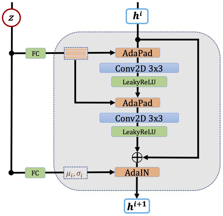
Time-Invariant Encoder. The encoder is implemented using 4 Conv 3D layers, each followed by
BatchNorm, LeakyReLU, and max-pooling. Note that theoretically, max-pooling is not perfectly shift
invariant since 2x2x2 max-pooling is equivariant to shifts of size 2 and only approximately invariant
to shifts of size 1. But standard convolutional architectures often include max-pooling layers to boost
performance. We convolve across spatial and temporal dimensions.
After that, we use a global mean-pooling layer and a fully connected layer to estimate the hidden
feature ẑc . The task parameter depends linearly on the hidden feature. We use a fully connected layer
to compute the parameter estimate ĉ. Since convolutions are equivariant to shift (up to boundary
frames) and mean pooling is invariant to shift, the encoder is shift-invariant. In practice, shifting the
time sequence one frame forward will add one new frame at the beginning and drop one frame at the
end. This creates some change in output value of the encoder. Thus, practically, the encoder is only
approximately shift-invariant.
Encoder Training. The encoder network g is trained first. To combat the loss of shift invariance
from the change from the boundary frames, we train the encoder using a time-invariant loss. Given
two training samples (x(i) , y (i) ) and (x(j) , y (j) ) and their task parameters c, we have loss
                        X                       X                             X
                Lenc =         kĉ − ck2 + α          kẑc(i) − ẑc(j) k2 + β   |kẑc(i) k − m|    (2)
                          c∼C                 i,j,c                     i,c

                                                             (i)
where ẑ (i) = g(x(i) ) and ẑ (j) = g(x(j) ) and ĉ(i) = W ẑc + b is an affine transformation of zc .
The first term kĉ − ck2 uses weak supervision of the task parameters whenever they are available.
Such weak supervision helps guide the learning of hidden feature zc for each task. While not all
parameters of the dynamical system are known, we can compute approximate values in the datum
c(i) based on our domain knowledge. For example, instead of the Reynolds number of the fluid flow,
we can use the average velocity as a surrogate for task parameters.
                    (i)     (j)
The second term kẑc − ẑc k2 is the time-shift invariance loss, which penalizes the changes in latent
variables between samples from different time steps. Since the time-shift invariance of convolution is
                                                                                            (i)
only approximate, this loss term drives the time-shift error even lower. The third term |kẑc k − m|
                                               (i)
prevents the encoder from generating small ẑc due to time-shift invariance loss. It also helps the
encoder to learn more interesting hidden features z, even in the absence of weak supervision.
Hidden Features. The encoder learns time-invariant hidden features. These hidden features resemble
the time-invariant dimensionless parameters [22] in physical modeling, such as Reynolds number in
fluid mechanics. The hidden features may also be viewed as partial disentanglement of the system
state. As suggested by [27, 37], our disentanglement method is guided by inductive bias and training
objectives. Unlike complete disentanglement, as in e.g. [30], in which the latent representation is
factored into time-invariant and time-varying components, we focus only on time-shift-invariance.
Nonetheless, the hidden features can control the forecaster which is useful for generalization.

2.4   Forecaster Network

The forecaster incorporates the hidden feature zc from the encoder and adapts to the specific fore-
casting task fc = f (·, zc ). In what follows, we use z for zc . We use two specialized layers, adaptive
instance normalization (AdaIN) and adaptive padding (AdaPad).
AdaIN has been used in neural style transfer [19, 17] to control generative networks. Here, AdaIN
may adapt for specific coefficients and external forces. We also introduce a new layer, AdaPad(x, z),
which is designed for encoding the boundary conditions of dynamical systems. In principle, the
backbone of the forecaster network can be any sequence prediction model. We use a design that is
similar to ResNet for spatiotemporal sequences.
AdaIN. We employ AdaIN to adapt the forecaster network. Denote the channels of input x by xi
and let µ(xi ) and σ(xi ) be the mean and standard deviation of channel i. For each AdaIN layer, a
particular style is computed s = (µi , σi )i = Az + b, where the linear map A and bias b are learned
weights. Adaptive instance normalization is then defined
                                                  xi − µ(xi )
                                        yi = σi               + µi .
                                                     σ(xi )

                                                      4
In essence, the channels are renormalized to the style s.
For dynamics forecasting, the hidden feature z encodes data analogous to the various coefficients of
a differential equation and external forces on the system. In numerical simulation of a differential
equation these coefficients enter as scalings of different terms in the equation and the external forces
are added to the combined force equation. Thus in our context AdaIN, which scales channels and
adds a global vector, is well-suited to injecting this information.
AdaPad. To complement AdaIN, we introduce AdaPad, which
encodes the boundary conditions of each specific dynamical system.
Generally when predicting dynamical systems, error is introduced
along the boundaries since it is unknown how the dynamics interact
with the boundary of the domain, and there may be unknown inflows
or outflows. In our method, the inferred hidden feature z may
contain the boundary information. AdaPad uses the hidden features
to compute the boundary conditions via a linear layer. Then it applies
the boundary conditions as padding immediately outside the spatial
domain in each layer, as shown in Fig. 3.
Forecaster Training. The forecaster network is trained separately
after the encoder. The kernels of the convolutions and the mappings
of the AdaIN and AdaPad layers are all trained simultaneously as
the forecaster network is trained. Denote the true state as y and the
predicted state as ŷ, we compute the loss per time step kŷ − yk2 for Figure 3: Illustration of the
each example. We accumulate the loss over different time steps and AdaPad operation.
generate multi-step forecasts in an autoregressive fashion.

3   Theoretical Analysis
The high-level idea of our method is to learn a good representation of the dynamics that generalizes
well across a heterogeneous domain, and then adapt this representation to make predictions on new
tasks. Our model achieves this by learning on multiple tasks simultaneously and then adapting to new
tasks with domain transfer. We provide an analysis for this procedure. See Appendix B for a longer
treatment with proofs.
Suppose we have K tasks {ck }K   k=1 ∼ C, each of which is sampled from a continuous parameter
space C. Here ck are the parameters of the task. For each task c, we have a collection of data Dc of
size n, sampled from µk , a shorthand for µck . Let D = ∪c∈C Dc be the union of data from all tasks.
Multi-task Learning
                  P Error. Our model performs multi-task representation learning [32] with joint
risk  = (1/K) k k , which is the average risk of each task k defined separately. Denote the
corresponding empirical risks ˆ and ˆk . We can bound the true risk  using the empirical risk ˆ and
Rademacher complexity R(F) of the hypothesis class F. The following theorem restates the main
result in [2] with simplified notations.
Theorem 3.1. [2] Assume the loss is bounded l ≤ 1/2. Given n samples each from K different
forecasting tasks µ1 , · · · , µk , then with probability at least 1 − δ, the following inequality holds for
each f ∈ F in the hypothesis class:
                                                                          r
                            1 X                1 X                           log 1/δ
                                     k (f ) ≤      ˆk (f ) + 2R(F) +
                           K                   K                              2nK
                              k                k

The following inequality compares the performance for multi-task learning to learning individual
tasks. Let Rk (F) be the Rademacher complexity for F over µk .
Lemma 3.2. The Rademacher complexity for multi-task learning is bounded as
                                                         K
                                                         X
                                      R(F) ≤ (1/K)             Rk (F).
                                                         k=1

We can now compare the bound from Theorem 3.1 with the bound obtained by considering each task
individually.

                                                     5
Proposition 3.3. Assume the loss is bounded l ≤ 1/2, then the generalization bound given by
considering each task individually is
                                             K
                                                     ! r
                                           1 X              log 1/δ
                        (f ) ≤ ˆ(f ) + 2     Rk (F) +             .                   (3)
                                           K                   2n
                                                  k=1

which is strictly looser than the bound from Theorem 3.1.

This helps explain why our multitask learning framework has better generalization than learning each
task independently. The shared data tightens the generalization bound.
Domain Adaptation Error. Since we test on c ∼ C outside the training set {ck }, we incur error
due to domain adaptation from the source domains µ1 , . . . , µK to target domain µc with µ being the
true distribution. Denote the corresponding empirical distributions of n samples per task by µ̂c . For
similar domains, the Wasserstein distance W1 (µc , µc0 ) is small. The bound from [43] applies well to
our setting as such:
                                                                      PK
Theorem 3.4 ([43],Theorem 2). Let λ = minf ∈F c (f ) + 1/K k=1 ck (f ) . There is N =
N (ζ, dim(D)) such that for n > N , for any hypothesis f , with probability at least 1 − δ,
               K                          K
                                                !
             1 X                       1 X          p              p           p
   c (f ) ≤      ck (f ) + W1 µ̂c ,        µ̂k + 2 log(1/δ)          1/n + 1/(nK) + λ.
             K                        K
                k=1                         k=1

Encoder versus Forecaster Error. Error from DyAd may result from either the encoder gφ or the
forecaster fθ . Our hypothesis space has the form {x 7→ fθ (x, gφ (x))} where φ and θ are the weights
of the encoder and forecaster respectively. Let X be the error over the entire domain X , that is, for
all c. Let enc (gφ ) = Ex∼X (L1 (g(x), gφ (x)) be the encoder error.
Proposition 3.5. Assume c 7→ supθ (fθ (·, c)) is Lipschitz continuous with Lipschitz constant γ. Then
we bound
                      X (fθ (·, gφ (·))) ≤ γenc (gφ ) + Ec∼C [c (fθ (x, c))]                    (4)
where the first term is the error due to the encoder incorrectly identifying the task and the second
term is the error due to the prediction network alone.

Together, we can bound the generalization error in terms of the empirical error of the forecaster on the
source domains, the Wasserstein distance between the source and target domains, and the empirical
error of the encoder; See proposition B.6 in Appendix.

4   Related Work
Learning Dynamical Systems. Deep learning models are gaining popularity for learning dynamical
systems [50, 9, 21, 6, 61, 54]. An emerging topic is physics-informed deep learning [42, 33, 28, 7,
10, 58, 5, 4, 26] which integrates inductive biases from physical systems to improve learning. For
example, [28] encoded Euler-Lagrange equation into the deep neural nets but focus on learning low-
dimensional trajectories. [35, 7] incorporated Koopman theory into the architecture. [33] used deep
neural networks to solve PDEs automatically with physical laws enforced in the loss functions. [57]
proposed a hybrid approach by marrying two well-established turbulent flow simulation techniques
with deep learning to produce better prediction of turbulence. However, these approaches deal with a
specific system dynamics instead of the meta-learning task in this work.
Meta-learning and Domain Adaptation. The aim of meta-learning [53] is to acquire generic
knowledge of different tasks for rapid generalization to new tasks. Based on how the meta-level
knowledge is extracted and used, meta-learning methods are classified into model-based [36, 47, 1,
40, 49], metric-based [56, 51] and gradient-based [11, 3, 46, 14, 63]. Most meta-learning approaches
are not designed for forecasting with a few exceptions. [40] designed a residual architecture for time
series forecasting with a meta-learning parallel. [1] proposed a modular meta-learning approach for
continuous control. But forecasting physical dynamics poses unique challenges to meta-learning as
we seek ways to encode physical knowledge into our model. DyAd is a meta-learning model since
the encoder can encode different tasks and extract high-level meta representations and the forecaster

                                                   6
then predicts across different systems without retraining. In statistical time series forecasting, meta-
learning [25, 52] was termed for model selection, which has a different objective from ours.
Style Transfer. Our approach is inspired by neural style transfer techniques. In style-transfer, a
generative network is controlled by an external style vector though adaptive instance normalization
between convolutional layers. Our hidden representation bears affinity with the “style” vector in
style transfer techniques. Rather than aesthetic style in images, our hidden representation encodes
time-invariant features. Style transfer initially appear in non-photorealistic rendering [23]. Recently,
neural style transfer [18] has been applied to image synthesis [13], videos generation [45], and
language translation [41]. For dynamical systems, [48] adapts texture synthesis to transfer the style
of turbulence for animation. [20] studies unsupervised generative modeling of turbulent flows but for
super-resolution reconstruction rather than forecasting.
Video Prediction. Our work is also related to video prediction. Conditioning on the historic observed
frames, video prediction models are trained to predict future frames, e.g., [31, 12, 62, 55, 39, 12,
59, 60, 24]. There is also conditional video prediction [38] which achieves controlled synthesis.
Many of these models are trained on natural videos from unknown physical processes. Our work is
substantially different because we do not attempt to predict object or camera motions. However, our
method can be potentially combined with video prediction models to improve generalization.

5     Experiments
We compare our model with a series of baselines on the multi-step forecasting with different dynamics.
We consider two testing scenarios: (1) dynamics with different initial conditions (test-future) and (2)
dynamics with different parameters such as external force (test-domain). The first scenario evaluates
the models’ ability to extrapolate into the future for the same task. The second scenario estimates the
capability of the models to generalize across different tasks.
We experiment on three datasets: sythetic turbulent flows, real-world sea surface temperature and
ocean currents data. These are difficult to forecast using numerical methods due to unknown external
forces and complex dynamics not fully captured by simplified mathematical models. For the weak
supervision c, we use the mean vorticity for turbulence and ocean currents, and mean temperature for
sea surface temperature. We defer the details of the datasets and experiments to Appendix A.2.

                  Turbulent Flows         Sea Temperature                        Ocean Currents
      Model
                  future     domain       future     domain             future                    domain
     ResNet      0.94±0.10   0.65±0.02   0.73±0.14   0.71±0.16   9.44±1.55 | 0.99±0.15   9.65±0.16 | 0.90±0.16
     U-Net       0.92±0.02   0.68±0.02   0.57±0.05   0.63±0.05   7.64±0.05 | 0.83±0.02   7.61±0.14 | 0.86±0.03
    PredRNN      0.75±0.02   0.75±0.01   0.67±0.12   0.99±0.07   8.49±0.01 | 1.27±0.02   8.99±0.03 | 1.69±0.01
    Mod-ind      1.13±0.03    ——–        1.25±0.35    ——–        10.1±0.27 | 0.97±0.16        ———–
    Mod-attn     0.63±0.12   0.92±0.03   0.89±0.22   0.98±0.17   8.08±0.07 | 0.76±0.11   8.31±0.19 | 0.88±0.14
     Mod-wt      0.58±0.03   0.60±0.07   0.65±0.08   0.64±0.09   10.1±0.12 | 1.19±0.72   8.11±0.19 | 0.82±0.19
    MetaNet      0.76±0.13   0.76±0.08   0.84±0.16   0.82±0.09   10.9±0.52 | 1.15±0.18   11.2±0.16 | 1.08±0.21
      MAML       0.63±0.01   0.68±0.02   0.90±0.17   0.67±0.04   10.1±0.21 | 0.85±0.06   10.9±0.79 | 0.99±0.14
    DyAd+ResNet 0.42±0.01 0.53±0.05 0.54±0.03        0.51±0.04   7.28±0.09 | 0.58±0.02   7.54±0.04 | 0.54±0.03
    DyAd+Unet 0.63±0.05 0.65±0.08 0.49±0.03          0.50±0.08   7.38±0.01 | 0.70±0.04   7.46±0.02 | 0.70±0.07

Table 1: Prediction RMSE on the turbulent flow and sea surface temperature datasets. Prediction
RMSE and ESE (energy spectrum errors) on the future and domain test sets of ocean currents dataset.

Baselines. We include several SoTA baselines from meta-learning, as well as common methods for
dynamics forecasting.

         • ResNet [16]: A widely adopted video prediction model [58].
         • U-net [44]: Originally developed for biomedical image segmentation, adapted for dynamics
           forecasting [10].
         • PredRNN [59]: A RNN-based spatiotemporal forecasting model.
         • Mod-ind: A simple baseline with independent CNN modules trained for different tasks.

                                                       7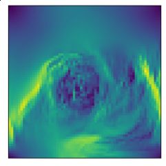
Figure 4: Target and predictions by ResNet, Modular-wt and DyAd at time 1, 5, 10 for turbulent
flows with buoyancy factors 9 (left) and 21 (right) respectively. We can see that DyAd can easily
generate predictions for various flows while ResNet and Modular-wt have trouble understanding
and disentangling buoyancy factors.
• Mod-attn: A modular meta-learning method which combines modules to generalize to new
tasks [1]. An attention mechanism is used to combine modules through the final output.
• Mod-wt: A modular meta-learning variant which uses attention weights to combine the
parameters of the convolutional kernels for new tasks.
• MetaNet [36]: A model-based meta-learning method which requires a few labels from test
tasks as a support set to adapt.
• MAML [11]: A popular gradient-based meta-learning approach. We replaced the classifier in
the original model with a ResNet for regression.
Both Mod-attn and Mod-wt have a convolutional encoder to generate attention weights. MetaNet
requires a few samples from test tasks as a support set and MAML needs adaptation retraining on test
tasks, while other models do not need any information from the test domains. See details about
baselines in Appendix A.2. To demonstrate the efficiency of DyAd, we tried using ResNet as well as
U-net as the forecaster in our framework.
Experiment Setup. For all datasets, we use a sliding window approach to generate samples of
sequences. For test-future, we train and test on the same tasks but different time steps. For test-
domain, we train and test on different tasks with an 80-20 split. All models are trained to make next
step prediction given the previous 20 steps as input. We forecast in an autoregressive manner to
generate multi-step ahead predictions. All results are averaged over 3 runs with random initialization.
Apart from the root mean square error (RMSE), we also report the energy spectrum error (ESE)
for ocean current prediction which quantifies the physical consistency. ESE indicates whether the
predictions preserve the correct statistical distribution and obey the energy conservation law, which is
a critical metric for physical consistency. See details about energy spectrum in Appendix A.3.
5.1 Experiment Results
Prediction Performance. Table 1 shows the RMSE of 10-step ahead predictions on two test sets of
turbulent flows, sea surface temperature and ocean currents. We observe that DyAd makes the most
accurate predictions
√ for both test sets of all datasets. Figure 4 shows the target and predictions of
velocity norm ( u2 + v 2 ) by ResNet, Modular-wt and DyAd at time 1, 5, 10 for turbulent flows
with buoyancy factors 9 (left) and 21 (right) respectively. We can see that DyAd can generate realistic
flows with the corresponding characteristics while the other two models have trouble understanding
and disentangling the buoyancy factor.
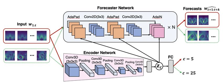
Table 1 also reports ESE on the ocean currents dataset for 10-step ahead predictions. DyAd not only
has small RMSE but also obtains the smallest ESE, suggesting it captures the statistical distribution
of ocean currents well. Figure 6 shows DyAd, ResNet, U-net, PredRNN predictions on an ocean
current sample in the future test set, and we see the shape of predictions by DyAd is closest to the
target. These results demonstrate that DyAd not only forecasts well but also accurately captures the
physical characteristics of the system. We also visualize the energy spectrum of target and predictions
8
Model          future       domain
    DyAd(ours)      0.42±0.01     0.53±0.02
      No_enc        0.63±0.03     0.60±0.02
    Wrong_enc       0.66±0.02     0.62±0.03
     End2End        0.45±0.01     0.54±0.01

 Figure 5: Ablation study: prediction RMSE         Figure 6: √
                                                             DyAd, ResNet, U-net, PredRNN veloc-
 of DyAd, DyAd without encoder, DyAd with          ity norm ( u2 + v 2 ) predictions on an ocean cur-
 encoder trained by wrong supervision c and        rent sample in the future test set.
 DyAd with end to end training.

by ResNet, U-net and DyAd on two test sets of ocean currents in Appendix A.4, Figure 11, with
DyAd being the closest to the target.
Ablation Study. We performed an ablation study of DyAd on the turbulence dataset to understand the
contribution of each component, shown in Table 5.1. We first remove the encoder from DyAd while
keeping the same forecaster network (No_enc). The resulting model degrades but still outperforms
ResNet. This demonstrates the effectiveness of AdaIN and AdaPad for forecasting.
Another notable feature of our model is the ability to infer tasks with weakly supervised signals c. It
is important to have a c that is related to the task domain. As an ablative study, we fed the encoder in
DyAd with a random c, leading to Wrong_enc. We can see that having the wrong supervision may
hurt the forecasting performance. We also tried to train DyAd end-to-end (End2End) but observed
worse performance. This validates our hypothesis about the significance of domain partitioning and
the two-stage training approach.
Controllable Forecast. DyAd infers the hidden fea-
tures from data, which allows direct control of the
latent space in the forecaster. We tried to vary the en-
coder input while keeping the forecaster input fixed.
Figure 7 shows the forecasts from DyAd when the
encoder is fed with flows having different buoyancy
factors c = 5, 15, 25. As expected, with higher buoy-
ancy factors, the predictions from the forecaster be-
come more turbulent. This demonstrates that the
encoder can successfully disentangle the latent repre-
sentation of difference tasks, and control the predic-
tions of the forecaster.

6   Conclusion                                         Figure 7: Outputs from DyAd while we vary
                                                       encoder input but keep the prediction network
We propose a model-based meta-learning method, input fixed. From left to right, the encoder is
DyAd to forecast physical dynamics. DyAd uses an fed with flow with different buoyancy factor
encoder to infer the parameters of the task and a c = 5, 15, 25. the prediction network input
prediction network to adapt and forecast giving the has fixed buoyancy c = 15.
inferred task. Our model can also leverage any weak
supervision signals that can help distinguish differ-
ent tasks, allowing the incorporation of additional
domain knowledge. On challenging turbulent flow prediction and real-world ocean temperature
and currents forecasting tasks, we observe superior performance of our model across heterogeneous
dynamics. Future work would consider non-grid data such as flows on a graph or a sphere.

                                                    9
References
 [1] Ferran Alet, Tomas Lozano-Perez, and L. Kaelbling.           Modular meta-learning.      ArXiv,
     abs/1806.10166, 2018.
 [2] Rie Kubota Ando, Tong Zhang, and Peter Bartlett. A framework for learning predictive
     structures from multiple tasks and unlabeled data. Journal of Machine Learning Research,
     6(11), 2005.
 [3] Marcin Andrychowicz, Misha Denil, Sergio Gomez Colmenarejo, M. W. Hoffman, D. Pfau,
     T. Schaul, and N. D. Freitas. Learning to learn by gradient descent by gradient descent. In
     Advances in Neural Information Processing Systems, 2016.
 [4] I. Ayed, Emmanuel de Bézenac, A. Pajot, J. Brajard, and P. Gallinari. Learning dynamical
     systems from partial observations. ArXiv, abs/1902.11136, 2019.
 [5] Ibrahim Ayed, Emmanuel De Bézenac, Arthur Pajot, and Patrick Gallinari. Learning partially
     observed PDE dynamics with neural networks, 2019.
 [6] Omri Azencot, N. Erichson, V. Lin, and Michael W. Mahoney. Forecasting sequential data
     using consistent koopman autoencoders. In International Conference on Machine Learning,
     2020.
 [7] Omri Azencot, N Benjamin Erichson, Vanessa Lin, and Michael Mahoney. Forecasting se-
     quential data using consistent koopman autoencoders. In International Conference on Machine
     Learning, pages 475–485. PMLR, 2020.
 [8] Jonathan Baxter. Theoretical models of learning to learn. In Learning to learn, pages 71–94.
     Springer, 1998.
 [9] Ricky TQ Chen, Yulia Rubanova, Jesse Bettencourt, and David Duvenaud. Neural ordinary dif-
     ferential equations. In Proceedings of the 32nd International Conference on Neural Information
     Processing Systems, pages 6572–6583, 2018.
[10] Emmanuel de Bezenac, Arthur Pajot, and Patrick Gallinari. Deep learning for physical pro-
     cesses: Incorporating prior scientific knowledge. In International Conference on Learning
     Representations, 2018.
[11] Chelsea Finn, P. Abbeel, and S. Levine. Model-agnostic meta-learning for fast adaptation of
     deep networks. In International Conference of Machine Learning, 2017.
[12] Chelsea Finn, Ian Goodfellow, and Sergey Leine. Unsupervised learning for physical interaction
     through video prediction. In Advances in neural information processing systems, pages 64–72,
     2016.
[13] Leon A Gatys, Alexander S Ecker, and Matthias Bethge. Image style transfer using convolutional
     neural networks. In Proceedings of the IEEE conference on computer vision and pattern
     recognition, pages 2414–2423, 2016.
[14] E. Grant, Chelsea Finn, S. Levine, Trevor Darrell, and T. Griffiths. Recasting gradient-based
     meta-learning as hierarchical bayes. ArXiv Preprint, abs/1801.08930, 2018.
[15] Abhishek Gupta, Russell Mendonca, YuXuan Liu, Pieter Abbeel, and Sergey Levine. Meta-
     reinforcement learning of structured exploration strategies. In Proceedings of the 32nd Interna-
     tional Conference on Neural Information Processing Systems, pages 5307–5316, 2018.
[16] Kaiming He, Xiangyu Zhang, Shaoqing Ren, and Jian Sun. Deep residual learning for image
     recognition. In Proceedings of the IEEE conference on computer vision and pattern recognition,
     pages 770–778, 2016.
[17] Xun Huang and Serge Belongie. Arbitrary style transfer in real-time with adaptive instance
     normalization. In Proceedings of the IEEE International Conference on Computer Vision, pages
     1501–1510, 2017.

                                                 10
[18] Yongcheng Jing, Yezhou Yang, Zunlei Feng, Jingwen Ye, Yizhou Yu, and Mingli Song. Neu-
ral style transfer: A review. IEEE transactions on visualization and computer graphics,
26(11):3365–3385, 2019.
[19] Tero Karras, Samuli Laine, and Timo Aila. A style-based generator architecture for generative
adversarial networks. In Proceedings of the IEEE/CVF Conference on Computer Vision and
Pattern Recognition, pages 4401–4410, 2019.
[20] Junhyuk Kim and Changhoon Lee. Deep unsupervised learning of turbulence for inflow
generation at various reynolds numbers. arXiv:1908.10515, 2019.
[21] J. Zico Kolter and Gaurav Manek. Learning stable deep dynamics models. In Advances in
Neural Information Processing Systems (NeurIPS), volume 32, pages 11128–11136, 2019.
[22] Josef Kunes. Dimensionless physical quantities in science and engineering. Elsevier, 2012.
[23] Jan Eric Kyprianidis, John Collomosse, Tinghuai Wang, and Tobias Isenberg. State of the"
art”: A taxonomy of artistic stylization techniques for images and video. IEEE transactions on
visualization and computer graphics, 19(5):866–885, 2012.
[24] Vincent Le Guen and Nicolas Thome. Disentangling physical dynamics from unknown factors
for unsupervised video prediction. In Computer Vision and Pattern Recognition (CVPR). 2020.
[25] Christiane Lemke and Bogdan Gabrys. Meta-learning for time series forecasting and forecast
combination. Neurocomputing, 73(10-12):2006–2016, 2010.
[26] Zongyi Li, Nikola Kovachki, Kamyar Azizzadenesheli, Burigede Liu, Kaushik Bhattacharya,
Andrew Stuart, and Anima Anandkumar. Fourier neural operator for parametric partial differen-
tial equations. International Conference on Learning Representations, 2021.
[27] Francesco Locatello, Stefan Bauer, Mario Lucic, Gunnar Raetsch, Sylvain Gelly, Bernhard
Schölkopf, and Olivier Bachem. Challenging common assumptions in the unsupervised learning
of disentangled representations. In international conference on machine learning, pages 4114–
4124. PMLR, 2019.
[28] Michael Lutter, Christian Ritter, and Jan Peters. Deep lagrangian networks: Using physics as
model prior for deep learning. In International Conference on Learning Representations, 2018.
[29] Gurvan Madec et al. NEMO ocean engine, 2015. Technical Note. Institut Pierre-Simon Laplace
(IPSL), France. https://epic.awi.de/id/eprint/39698/1/NEMO_book_v6039.pdf.
[30] Armand Comas Massague, Chi Zhang, Zlatan Feric, Octavia Camps, and Rose Yu. Learning
disentangled representations of video with missing data. arXiv preprint arXiv:2006.13391,
2020.
[31] Michael Mathieu, Camille Couprie, and Yann LeCun. Deep multi-scale video prediction beyond
mean square error. arXiv preprint arXiv:1511.05440, 2015.
[32] Andreas Maurer, Massimiliano Pontil, and Bernardino Romera-Paredes. The benefit of multitask
representation learning. Journal of Machine Learning Research, 17(81):1–32, 2016.
[33] George E Karniadakis Maziar Raissi, Paris Perdikaris. Physics-informed neural networks: A
deep learning framework for solving forward and inverse problems involving nonlinear partial
differential equations. Journal of Computational Physics, 378:686–707, 2019.
[34] Mehryar Mohri, Afshin Rostamizadeh, and Ameet Talwalkar. Foundations of machine learning.
MIT press, 2018.
[35] Jeremy Morton, Antony Jameson, Mykel J. Kochenderfer, and Freddie Witherden. Deep
dynamical modeling and control of unsteady fluid flows. In Advances in Neural Information
Processing Systems (NeurIPS), 2018.
[36] Tsendsuren Munkhdalai and Hong Yu. Meta networks. Proceedings of machine learning
research, 70:2554–2563, 2017.
11[37] Weili Nie, Tero Karras, Animesh Garg, Shoubhik Debhath, A. Patney, Ankit B. Patel, and
Anima Anandkumar. Semi-supervised stylegan for disentanglement learning. In International
Conference on Machine Learning, 2020.
[38] Junhyuk Oh, Xiaoxiao Guo, Honglak Lee, Richard Lewis, and Satinder Singh. Action-
conditional video prediction using deep networks in atari games. In Proceedings of the 28th
International Conference on Neural Information Processing Systems-Volume 2, pages 2863–
2871, 2015.
[39] Sergiu Oprea, P. Martinez-Gonzalez, A. Garcia-Garcia, John Alejandro Castro-Vargas, S. Orts-
Escolano, J. Garcia-Rodriguez, and Antonis A. Argyros. A review on deep learning techniques
for video prediction. ArXiv, abs/2004.05214, 2020.
[40] Boris N Oreshkin, Dmitri Carpov, Nicolas Chapados, and Yoshua Bengio. N-beats: Neural
basis expansion analysis for interpretable time series forecasting. In International Conference
on Learning Representations, 2019.
[41] Shrimai Prabhumoye, Yulia Tsvetkov, Ruslan Salakhutdinov, and Alan W Black. Style transfer
through back-translation. In Proceedings of the 56th Annual Meeting of the Association for
Computational Linguistics (Volume 1: Long Papers), pages 866–876, 2018.
[42] Maziar Raissi, Paris Perdikaris, and George Em Karniadakis. Physics informed deep learn-
ing (part i): Data-driven solutions of nonlinear partial differential equations. arXiv preprint
arXiv:1711.10561, 2017.
[43] Ievgen Redko, Amaury Habrard, and Marc Sebban. Theoretical analysis of domain adaptation
with optimal transport. In Joint European Conference on Machine Learning and Knowledge
Discovery in Databases, pages 737–753. Springer, 2017.
[44] Olaf Ronneberger, Philipp Fischer, and Thomas Brox. U-net: Convolutional networks for
biomedical image segmentation. In International Conference on Medical image computing and
computer-assisted intervention, pages 234–241. Springer, 2015.
[45] Manuel Ruder, Alexey Dosovitskiy, and Thomas Brox. Artistic style transfer for videos. In
German conference on pattern recognition, pages 26–36. Springer, 2016.
[46] Andrei A. Rusu, Dushyant Rao, Jakub Sygnowski, Oriol Vinyals, Razvan Pascanu, Simon
Osindero, and Raia Hadsell. Meta-learning with latent embedding optimization. In International
Conference on Learning Representations, 2019.
[47] A. Santoro, Sergey Bartunov, M. Botvinick, Daan Wierstra, and T. Lillicrap. Meta-learning
with memory-augmented neural networks. In ICML, 2016.
[48] Syuhei Sato, Yoshinori Dobashi, Theodore Kim, and Tomoyuki Nishita. Example-based
turbulence style transfer. ACM Transactions on Graphics (TOG), 37(4):1–9, 2018.
[49] Sungyong Seo, Chuizheng Meng, Sirisha Rambhatla, and Y. Liu. Physics-aware spatiotemporal
modules with auxiliary tasks for meta-learning. ArXiv, abs/2006.08831, 2020.
[50] Xingjian Shi, Zhihan Gao, Leonard Lausen, Hao Wang, D. Yeung, W. Wong, and Wang chun
Woo. Deep learning for precipitation nowcasting: A benchmark and a new model. In Advances
in neural information processing systems, 2017.
[51] J. Snell, Kevin Swersky, and R. Zemel. Prototypical networks for few-shot learning. In Advances
in Neural Information Processing Systems, 2017.
[52] Thiyanga S Talagala, Rob J Hyndman, George Athanasopoulos, et al. Meta-learning how to
forecast time series. Technical report, Monash University, Department of Econometrics and
Business Statistics, 2018.
[53] Sebastian Thrun and Lorien Pratt. Learning to learn: Introduction and overview. In Learning to
learn, pages 3–17. Springer, 1998.
12[54] Jonathan Tompson, Kristofer Schlachter, Pablo Sprechmann, and Ken Perlin. Accelerating
Eulerian fluid simulation with convolutional networks. In ICML’17 Proceedings of the 34th
International Conference on Machine Learning, volume 70, pages 3424–3433, 2017.
[55] Ruben Villegas, Jimei Yang, Seunghoon Hong, Xunyu Lin, and Honglak Lee. Decomposing
motion and content for natural video sequence prediction. In International Conference on
Learning Representations (ICLR), 2017.
[56] Oriol Vinyals, Charles Blundell, T. Lillicrap, K. Kavukcuoglu, and Daan Wierstra. Matching
networks for one shot learning. In NIPS, 2016.
[57] Rui Wang, Karthik Kashinath, Mustafa Mustafa, Adrian Albert, and Rose Yu. Towards physics-
informed deep learning for turbulent flow prediction. In Proceedings of the 26th ACM SIGKDD
International Conference on Knowledge Discovery & Data Mining, pages 1457–1466, 2020.
[58] Rui Wang, Robin Walters, and Rose Yu. Incorporating symmetry into deep dynamics models
for improved generalization. arXiv preprint arXiv:2002.03061, 2020.
[59] Yunbo Wang, Mingsheng Long, Jianmin Wang, Zhifeng Gao, and Philip S Yu. PredRNN:
Recurrent neural networks for predictive learning using spatiotemporal LSTMs. In Advances in
Neural Information Processing Systems, pages 879–888, 2017.
[60] Yunbo Wang, Haixu Wu, Jianjin Zhang, Zhifeng Gao, Jianmin Wang, Philip S Yu, and Ming-
sheng Long. PredRNN: A recurrent neural network for spatiotemporal predictive learning,
2021.
[61] You Xie, Erik Franz, Mengyu Chu, and Nils Thuerey. tempoGAN: A temporally coherent,
volumetric GAN for super-resolution fluid flow. ACM Transactions on Graphics (TOG),
37(4):95, 2018.
[62] Tianfan Xue, Jiajun Wu, Katherine Bouman, and Bill Freeman. Visual dynamics: Probabilistic
future frame synthesis via cross convolutional networks. In Advances in neural information
processing systems (NeurIPS), pages 91–99, 2016.
[63] Huaxiu Yao, Ying Wei, Junzhou Huang, and Zhenhui Li. Hierarchically structured meta-learning.
In International Conference on Machine Learning, pages 7045–7054. PMLR, 2019.
[64] Jaesik Yoon, Taesup Kim, Ousmane Dia, Sungwoong Kim, Yoshua Bengio, and Sungjin Ahn.
Bayesian model-agnostic meta-learning. In Proceedings of the 32nd International Conference
on Neural Information Processing Systems, pages 7343–7353, 2018.
[65] David Zoltowski, Jonathan Pillow, and Scott Linderman. A general recurrent state space
framework for modeling neural dynamics during decision-making. In International Conference
on Machine Learning, pages 11680–11691. PMLR, 2020.
13A Implementation Details
A.1 Model Design
The prediction network ŷ = f (x, z) is composed of 8 blocks. Each block operates on a hidden state
h(i) of shape B × H × W × Cin and yields a new hidden state h(i+1) of the shape B × H × W × Cout .
The first input is h0 = x and the final output is computed from the final hidden state as ŷ =
Conv2D(h(8) ). We define each block as
a(i) = σ(Conv2D(AdaPad(h(i) , z)))
b(i) = σ(Conv2D(AdaPad(a(i) , z))) + h(i)
hi+1 = AdaIN(b(i) , z)
as illustrated in Figure 3.
Figure 8: Detail of the DyAd encoder. The conv3D layers are shift equivariant and global mean
pooling is shift invariant. The network is approximately invariant to spatial and temporal shifts.
A.2 Experiment Details
A.2.1 Datasets
Turbulent Flow with Varying Buoyancy. We generate a synthetic dataset of turbulent flows with a
numerical simulator, PhiFlow1 . It contains 64×64 velocity fields of turbulent flows in which we vary
the buoyant force acting on the fluid from 1 to 25. Each buoyant force corresponds to a forecasting
task and there are 25 tasks in total. We use the mean vorticity of each task as partial supervision c as
we can directly calculate it from the data. Vorticity can characterize formation and circular motion of
turbulent flows.
Sea Surface Temperature. We evaluate on a real-world sea surface temperature data generated
by the NEMO ocean engine [29]2 . We select an area from Pacific ocean range from 01/01/2018
1
https://github.com/tum-pbs/PhiFlow
2
The data are available at https://resources.marine.copernicus.eu/?option=com_csw&view=
details&product_id=GLOBAL_ANALYSIS_FORECAST_PHY_001_024
14to 12/31/2020. The corresponding latitude and longitude are (-150∼-120, -20∼-50). This area is
then divided into 25 64×64 subregions, each is a task since the mean temperature varies a lot along
longitude and latitude. For the encoder training, we use season as an additional supervision signal
besides the mean temperature of each subregion. In other words, the encoder should be able to infer
the mean temperature of the subregion as well as to classify four seasons given the temperature series.
Ocean Currents. We also experiment with the velocity fields of ocean currents from the same region
and use the same task division as the sea surface temperature data set. Similar to the turbulent flow
data set, we use the mean vorticity of each subregion as the weak-supervision signal.
For fair comparison, we set these models to have equal capacity as DyAd in terms of number of
parameters. Hyperparameters including learning rate, input length and the number of steps of
accumulated loss for training are tuned on validation sets.
A.2.2 Baselines.
Modular-attn has a convolutional encoder f that takes the same input x as each module M to
Pm
generate attention weights, l=1 Pmexp[f (x)(l)]
Ml (x). Modular-wt also has the same encoder
k=1 exp[f (x)(k)]
but to generate weights for combining the convolution parameters of all modules. We use additional
samples of up to 20% of the test set from test tasks. MetaNet uses these as a support set. MAML is
retrained on these samples for 10 epoch for adaptation.
A.2.3 Hyperparameter tuning.
We tuned learning rate (1e-3∼1e-5), batch size (16∼64), the number of accumulated errors for
backpropogation (2∼5), and hidden size (64∼512) of Modular Networks and Meta-Nets. We fixed
the number of historic input frames as 20. When we trained the encoder on turbulent flows and sea
surface temperature, we used α = 1 and β = 1. For ocean currents, we used α = 0.2 and β = 0.2.
We performed all our experiments on 4 V100 GPUs.
A.2.4 Model Capacity.
Table 2 displays the number of parameters of each tuned model.
ResNet U-net PredRNN Mod-ind Mod-attn Mod-wt MetaNets MAML DyAd
20.32 9.69 27.83 13.01 13.19 13.19 9.63 20.32 15.60
Table 2: The number of parameters of each model.
Figure 9: Detail of one block of the forecaster network.
15Figure 10: Spectrum plot
A.3 Turbulence kinetic energy spectrum
The turbulence kinetic energy spectrum E(k) is related to the mean turbulence kinetic energy as
Z ∞
E(k)dk = ((u0 )2 + (v 0 )2 )/2,
0
T
1X
(u0 )2 = (u(t) − ū)2 ,
T t=0
where the k is the wavenumber and t is the time step. Figure 10 shows a theoretical turbulence
kinetic energy spectrum plot. The spectrum can describe the transfer of energy from large scales of
motion to the small scales and provides a representation of the dependence of energy on frequency.
Thus, the Energy Spectrum Error can indicate whether the predictions preserve the correct statistical
distribution and obey the energy conservation law. A trivial example that can illustrate why we need
ESE is that if a model simply outputs moving averages of input frames, the accumulated RMSE of
predictions might not be high but the ESE would be really big because all the small or even medium
eddies are smoothed out.
A.4 Additional Results
Figure 11: The energy spectrum of target and predictions by ResNet, U-net and DyAd on future test
set (left) and domain test set (right) of ocean currents.
B Theoretical Analysis
The high-level idea of our method is to learn a good representation of the underlying dynamics from
multiple tasks, and then transfer this representation to a target task (domain adaptation).
16Definition 1 (Forecasting task). Each forecasting task xt+1 = f (xt , . . . ) is to learn a conditional
distribution µ over the system states µ : p(xt+1 |xt , . . . ) conditioned on the sequence of previous
states where µ is a probability measure.
In our setting, we have K tasks, each of which is sampled from a continuous, finite space {ck } ∼ C.
Let µk be the corresponding conditional probability measure p(xt , . . . , x1 |ck ). For each task ck , we
have a collection of n series as realizations from the dynamical system Xk = {(xt , . . . , x1 ; ck )(i) }ni=1
S from µk . The semicolon here represents the system behavior in a specific domain ck . Let
sampled
X = Xk be the union of samples over all tasks.
k
In practice, we often have some intuition of the variables that dictate the domain. Therefore, we have
two possible scenarios for the role of c in dynamical systems:
1. c fully distinguishes the task: the differences in Xk can be completely explained by the
differences in ck ;
2. c partially distinguishes the task: a more realistic scenario where we only have partial
knowledge of the domain. There exist latent variables z 0 that need to be inferred from raw
data. Together z = [c, z 0 ] can describe the behavior of the system in a domain.
We assume Scenario 1, which resembles the multi-task representation learning setting [32] with joint
true risk over all tasks and individual task true risk k defined respectively
K
1 X h
(i)
i
(f ) = k (f ), k (f ) = Ex(i) ∼µ l f xk (5)
K k k
k=1
and corresponding empirical risks
K
1 X
ˆ(f, X) = l(f (Xk )), ˆk (f, Xk ) = l(f (Xk )),
K
k=1
where l is a loss function.
B.1 Multi-Task Learning Error
We want to bound the true loss using the empirical loss ˆ and Rademacher complexity of the
hypothesis class F. We can use the classic results from [2]. Define empirical Rademacher complexity
for samples from all tasks as
" K n
!#
1 X X (i) (i)
R̂X (F) = Eσ sup σk l(f (xk )) (6)
f ∈F nK i=1 k=1
(i) (i)
where {σk } are independent binary variables σk ∈ {−1, 1}. The true Rademacher complexity is
then defined R(F) = EX (R̂X (F)).
The following theorem restates the main result from [2]. We simplify the statement by using the
Rademacher complexity rather than the set cover number argument used in the original proof.
Theorem B.1. [2] Given data from K different forecasting tasks µ1 , · · · , µk and f in hypothesis
class F, for some constant C with probability at least 1 − δ, the following inequality holds:
r
1 X 1 X log 1/δ
k (f ) ≤ ˆk (f ) + 2R(F) + C . (7)
K K nK
k k
√
If we assume the loss is bounded l ≤ 1/2, then we may take C = 1/ 2.
(i)
Proof. Consider {xk } as independent random variables. For a function φ that satisfies
|φ(x(1) , · · · , x(i) , · · · x(n) ) − φ(x(1) , · · · , x̃(i) , · · · x(n) )| ≤ ci
17by McDiarmid’s inequality, we have
2t2
(1) (n)
p φ(x ,··· ,x ) − E[φ] ≥ t ≤ exp − P 2 .
i ci
Applying this inequality to the max difference Q(X) = supf ∈F [(f )−ˆ
(f, X)], then with probability
at least 1 − δ, we have
r
log 1/δ
Q(X) − EX [Q(X)] ≤ C
nK
√ on the bounds ci . If the loss l ≤ 1/2, then |Q| ≤ 1/2 and so we can
where C is a constant depending
take ci = 1 leading to C = 1/ 2. A standard computation (see [34], Theorem 3.3) using the law of
total expectation shows EX [Q(X)] ≤ 2R(F), which finishes the proof.
We can use this to compare the generalization error of multi-task learning versus that of learning
the individual tasks. The following inequality compares the Rademacher complexity for multi-task
learning to that of individual task learning. Denote R̂Xk and Rk the empirical and true Rademacher
complexity for F over µk .
Lemma B.2. The Rademacher complexity for multi-task learning is bounded R(F) ≤
PK
(1/K) k=1 Rk (F).
Proof. We compute the empirical Rademacher complexity,
" K n
!# "K n
!#
1 X X (i) (i) X 1 X (i) (i)
R̂X (F) = Eσ sup σk l f x k ≤ Eσ sup σ l f xk
f ∈F nK f ∈F nK i=1 k
k=1 i=1 k=1
K
" n
!#
1 X 1 X (i) (i)
= Eσ sup σ l f xk
K f ∈F n i=1 k
k=1
K
" n
!#
1 X 1 X (i) (i)
= Eσk sup σ l f xk
K f ∈F n i=1 k
k=1
K
1 X
= R̂Xk (F)
K
k=1
The first inequality follows from the sub-additivity of the supremum function. The next equality is
due to the fact positive scalars commute with supremum, and by the linearity of expectation. The
expectation Eσ reduces to the expectation Eσk over only those Rademacher variables appearing
inside the expectation. Rk (F) is the Rademacher complexity of the function on the individual task k.
Taking expectation over all samples X gives the result.
It is instructive to compare the bound from Theorem B.1 with the generalization error bound obtained
by considering each task individually.
Proposition B.3. Assume n = nk for all tasks k and the loss l is bounded l ≤ 1/2, then the
generalization bound given by considering each task individually is
K
! r
1 X log 1/δ
(f ) ≤ ˆ(f ) + 2 Rk (F) + . (8)
K 2n
k=1
which is strictly looser than the bound from Theorem B.1 under the same assumptions.
This result helps to explain why our multitask learning framework has better generalization than
learning each task independently. The shared data tightens the generalization bound.
18You can also read