Can Existing Theory Predict the Response of Tropical Cyclone Intensity to Idealized Landfall?
←
→
Page content transcription
If your browser does not render page correctly, please read the page content below
Generated using the official AMS LATEX template—two-column layout. FOR AUTHOR USE ONLY, NOT FOR SUBMISSION!

                                                                        MANUSCRIPT SUBMITTED TO        JOURNAL OF THE ATMOSPHERIC SCIENCES

                                                      Can Existing Theory Predict the Response of Tropical Cyclone Intensity to Idealized
                                                                                         Landfall?
                                                                                                   J IE C HEN* AND DANIEL R. C HAVAS
arXiv:2102.04583v1 [physics.ao-ph] 9 Feb 2021

                                                                                                   Purdue University, West Lafayette, Indiana

                                                                                                                 ABSTRACT

                                                                   Tropical cyclones cause significant inland hazards, including wind damage and freshwater flooding, that
                                                                depend strongly on how storm intensity evolves at and after landfall. Existing theoretical predictions for the
                                                                time-dependent and equilibrium response of storm intensity have been tested over the open ocean but not yet
                                                                to be applied to storms after landfall. Recent work examined the transient response of the tropical cyclone low-
                                                                level wind field to instantaneous surface roughening or drying in idealized axisymmetric f -plane simulations.
                                                                Here, experiments testing combined surface roughening and drying with varying magnitudes of each are used
                                                                to test theoretical predictions for the intensity response. The transient response to combined surface forcings
                                                                can be reproduced by the product of their individual responses, in line with traditional potential intensity
                                                                theory. Existing intensification theory is generalized to weakening and found capable of reproducing the
                                                                time-dependent inland intensity decay. The initial (0-10min) rapid decay of near-surface wind caused by
                                                                surface roughening is not captured by existing theory but can be reproduced by a simple frictional spin-down
                                                                model, where the decay rate is a function of surface roughness. Finally, the theory is shown to compare well
                                                                with the prevailing empirical decay model for real-world storms. Overall, results indicate the potential for
                                                                existing theory to predict how tropical cyclone intensity evolves after landfall.

                                                1. Introduction                                                            ily generalized to a more fundamental understanding of
                                                                                                                           the storm response to landfall over a wide range of land
                                                   Landfalling tropical cyclones (TCs) bring tremendous
                                                                                                                           surfaces. An alternative approach is the use of empirical
                                                damage to both coastal and inland regions (Rappaport
                                                2000, 2014; Villarini et al. 2014). These damages may                      models or probabilistic models to predict storm inland in-
                                                change in the future should TCs move and/or decay more                     tensity decay, which may incorporate both storm and en-
                                                slowly in a warming climate (Kossin 2018, 2019; Li and                     vironmental parameters (Kaplan and DeMaria 1995, 2001;
                                                Chakraborty 2020). Therefore, a credible estimation of                     Vickery and Twisdale 1995; Vickery 2005; DeMaria et al.
                                                TC intensity decay after landfall is essential for hazard                  2006; Bhowmik et al. 2005). Empirical models mod-
                                                prediction. Having a physically-based theoretical solu-                    els have been incorporated into the Statistical Hurricane
                                                tion for the storm intensity response to landfall could help               Intensity Prediction Scheme for the Atlantic and east-
                                                improve risk assessment, both in real time for impending                   ern Pacific Oceans (DeMaria and Kaplan 1994; DeMaria
                                                landfall events and in climatological studies (Jing and Lin                et al. 2005) and Statistical Typhoon Intensity Prediction
                                                2020; Xi et al. 2020). However, the underlying physics                     Scheme for the western North Pacific (Knaff et al. 2005),
                                                governing this post-landfall response are not well under-                  and have been tested for landfalling hurricanes along the
                                                stood, and no such predictive theory currently exists.                     South China Coast (Wong et al. 2008). Statistical models
                                                   Past research has examined TC intensity at and after                    have also been incorporated into hurricane risk assessment
                                                landfall via numerical simulations of historical cases and                 models in the context of climate change (Vickery et al.
                                                statistical models. Numerical models have limited capac-                   2000; Emanuel et al. 2006; Jing and Lin 2020). However,
                                                ity to predict post-landfall intensity due to the difficulty               current statistical models do not incorporate the physics of
                                                of capturing the physics over complex terrain, which is                    hurricane intensity decay over land, and their accuracy is
                                                not necessarily improved by increasing model resolution                    limited by the data collected to train the model. Thus, em-
                                                or assimilating observational data (Shen 2005; Liu et al.                  pirical models offer limited fundamental understanding of
                                                2017). Moreover, site-specific case studies are not read-                  the inland decay of hurricane intensity, particularly under
                                                                                                                           a changing climate.
                                                                                                                              Physically-based theoretical models are formulated for
                                                   * Corresponding author address: Jie Chen, Purdue University, 550
                                                Stadium Mall Dr., West Lafayette, IN 47907.
                                                                                                                           TCs over the ocean. Quasi-steady state theories for the
                                                E-mail: chen2340@purdue.edu

                                                Generated using v4.3.2 of the AMS LATEX template                       1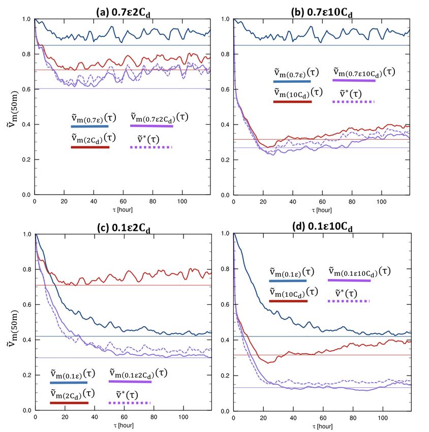
2                 MANUSCRIPT SUBMITTED TO      JOURNAL OF THE ATMOSPHERIC SCIENCES

tropical cyclone date back to Lilly and Emanuel (1985,          applied to predict the intensity response to surface forc-
unpublished manuscript), Shutts (1981), Emanuel (1986,          ings. Section 3 describes our idealized simulation experi-
hereafter referred to E86). More recently, theory now ex-       ments that are used to test the theory. Section 4 presents
ists for TC intensification over the ocean (Emanuel (2012),     our results addressing the research questions. Section 5
hereafter referred to E12) that was found to compare well       summarizes key results, limitations, and avenues for fu-
with an axisymmetric model simulation (Emanuel 2018).           ture work.
However, due to the complexities in the transition from
ocean to land, research has yet to develop a theory for post-   2. Theory
landfall decay that account for the basic physics of the re-
                                                                   This work examines two existing theories that predict
sponse of a tropical cyclone to landfall. Meanwhile, the
                                                                the equilibrium intensity (E86) and the time-dependent in-
potential for existing theoretical models for storms over
                                                                tensity change (E12) of a tropical cyclone. The original
the ocean to be applied after landfall has yet to be ex-
                                                                motivation of such theories is for storms over the ocean.
plored. Therefore, testing existing theories against ideal-
                                                                CC20 found that the equilibrium response of a mature TC
ized landfalls is a natural step to understand how known
                                                                to instantaneous surface roughening or drying followed
physics can or cannot explain the response of TC intensity
                                                                the response predicted by E86 theory closely. This work
after landfall. This is the focus of our work.
                                                                expands on CC20 by testing both the E86 and E12 theory
   Chen and Chavas (2020, hereafter referred to CC20)
                                                                and generalizes the experiments to simultaneous surface
idealized landfall as a transient response of a mature ax-
                                                                roughening and drying. This section reviews each theoret-
isymmetric TC to instantaneous surface forcing: surface
                                                                ical prediction and demonstrates how they can be formu-
roughening or drying, each over a range of magnitudes.
                                                                lated to apply to idealized landfall experiments.
They tested the response to each forcing individually and
showed that each ultimately causes the storm to weaken
                                                                a. Equilibrium intensity prediction: E86
but via different mechanistic pathways. They further
showed that the final equilibrium intensity in response to         Potential intensity is a theoretical upper-bound for the
each forcing can be predicted by E86 potential intensity        tropical cyclone intensity in a given thermodynamic envi-
theory. A logical next step is to test whether the transient    ronment. This theory is formulated by idealizing a mature
intensity response can be predicted by existing theory and,     tropical cyclone as a Carnot heat engine, where entropy
further, whether results can be generalized to any combi-       fluxes from the ocean surface are used to maintain the cir-
nation of surface drying and roughening adjusted simulta-       culation against surface frictional dissipation. Potential in-
neously. Both outcomes would be more directly relevant          tensity Vp is expressed as (Bister and Emanuel 1998),
to a wide range of inland surfaces felt by storms in real-                                 r
world landfalls.                                                                              Ck
                                                                                     Vp =        η(4k)                     (1)
   Therefore, in this work, both steady-state intensity                                       Cd
theory (E86) and time-dependent intensity change the-
ory (E12) are tested against different sets of simula-          where
                                                                                             TST − Tt pp
tions where surface roughness and wetness are individ-                                 η=                                   (2)
                                                                                                Tt pp
ually/simultaneously modified instantaneously beneath a
mature axisymmetric tropical cyclone. We seek to answer                 4k = C p (TST − Ta ) + εLv (q∗ (TST ) − qa (Ta ))   (3)
the following research questions:                               Ck and Cd are bulk exchange coefficient for surface en-
    1. Can traditional potential intensity theory predict the   thalpy and momentum, respectively; 4k is the difference
       equilibrium response to simultaneous surface drying      between the saturation enthalpy of the ocean surface and
       and roughening?                                          the enthalpy of the overlying near-surface air; TST is the
                                                                surface temperature, Ta is the temperature of air overlying
    2. Can the transient response to simultaneous drying        the surface; Tt pp is the tropopause temperature; Lv is the
       and roughening be predicted from the responses to        enthalpy of vaporization; C p is the specific heat capacity
       each forcing individually?                               of air; q∗ is the saturation mixing ratio of the ocean surface
                                                                at the local surface pressure; qa is the mixing ratio of air
    3. Can existing intensification theory predict the tran-    overlying the ocean surface; and ε is surface evaporative
       sient decay response to surface drying and/or rough-     fraction, which is taken as 1 over ocean surface. This for-
       ening?                                                   mulation includes the effect of dissipative heating, which
    4. Do the theories work for the intensity both near the     results in the tropopause temperature replacing the surface
       surface and near the top of the boundary layer?          temperature in the denominator of the Carnot efficiency
                                                                factor (Bister and Emanuel 1998).
   This paper is structured as follows. Section 2 reviews          For inland storms, where the underlying surface has a
the relevant theories and demonstrates how they may be          higher Cd (i.e., a rougher surface) and smaller ε (i.e., a
MANUSCRIPT SUBMITTED TO             JOURNAL OF THE ATMOSPHERIC SCIENCES                                                      3

drier surface), Eq.(1) would predict a weaker maximum
sustained wind speed compared to the ocean environment.
Thus, we define the response of Vp to any given surface
forcing as the ratio of its post-forcing value to its initial
pre-forcing value. Following CC20, the predicted Vp re-
sponse to surface roughening is given by
                                         s
                           Vp(Cd )             Cd
               Ṽp(Cd ) =           =                            (4)
                          Vp(CT RL)          (Cd )EXP

or surface drying given by
                                 s
                   Vp(ε)             C p 4T + (ε)EXP Lv 4q
      Ṽp(ε) =               =                                   (5)
                 Vp(CT RL)                    4k

where (Cd )EXP and (ε)EXP are the modified value of each
respective surface property parameter, representing vari-
ous magnitudes of surface roughening or drying. Vp(CT RL)
is the potential intensity of a Control pre-landfall TC (de-
fined in Section 3). As discussed in CC20, using normal-
ized responses of Vp can generalize the results to any ma-
ture storm intensity and also minimizes sensitivities as-
                                                                           F IG . 1. Normalized intensity decay predicted by E12 theory with
sociated with the precise definition of Vp . CC20 demon-               vm (0) = 100 ms−1 : (a) varying ṽ f with h = 5km, for v f =80%, 60%,
strated that the final equilibrium intensity response in ide-          40%, 20% and 0% of initial intensity (Eq.(10)); (b) varying h with ṽ f =
alized simulations closely follows this prediction.                    0 (Eq.(11)). Note that for ṽ f = 0, intensity reaches zero only as τ → ∞.
   Here we expand this approach to simultaneous surface
drying and roughening, i.e.
                                                                       b. Transient intensity prediction: E12
                           q
                                  Ck                                      E12 presents a theory for the time-dependent intensi-
              Vp(Cd ε)         (Cd )EXP η(C p 4T    + (ε)EXP Lv 4q)
Ṽp(Cd ε) =            =                 q                             fication of a TC, based on the role of outflow turbulence
              VpCT RL                        Ck
                                                                       in setting the radial distribution of low-level entropy pro-
                                             Cd η4k
                                                            (6)        posed in Emanuel and Rotunno (2011). The equation is
Mathematically, Eq.(6) indicates that the equilibrium in-              given by
tensity response to simultaneous forcing, Ṽp(Cd ε) , is simply                                                  Ck v f
                                                                                           vm (τ) = v f tanh (          τ)          (9)
the product of the individual equilibrium responses, Ṽp(Cd )                                                     2h
and Ṽp(ε) , i.e.                                                      with initial condition vm = 0 at τ = 0, where vmax is the fi-
                                                                       nal steady-state maximum wind speed and h is a constant
                                                                       boundary layer depth scale within the eyewall. Ramsay
                     Ṽp(Cd ε) = Ṽp(Cd )Ṽp(ε) .                (7)   et al. (2020) generalized this equation to predict intensifi-
                                                                       cation from a non-zero initial intensity. Here we further
The implication is that the response to any combination of             generalize Eq.(9) to represent the decay from an initial in-
surface roughening and drying may be predictable from                  tensity vm (0) to a weaker equilibrium intensity v f (see Ap-
the responses to each individual forcing. Inspired by                  pendix). This can be written in a form normalized by the
Eq.(7), the complete time-dependent response of storm in-              initial intensity given by
tensity ṽm(Cd ε) (τ) to simultaneous surface roughening and
drying is hypothesized as the product of the individual                                                 Ck v f
                                                                              ṽm(th) (τ) = ṽ f coth          τ + tanh−1 (ṽ f )  (10)
transient responses, i.e.                                                                                2h
                                                                                              v     (τ)               v
          ṽm(Cd ε) (τ) ≈ ṽ∗ (τ) = ṽm(Cd ) (τ)ṽm(ε) (τ)       (8)   where ṽm(th) (τ) = m(th)                  f
                                                                                             vm (0) and ṽ f = vm (0) . We use the sub-
                                                                       script th to denote the intensity predicted by theory. Exam-
The above outcome would have significant practical bene-               ples of the theoretical prediction of Eq.(10) are presented
fits for understanding the response to a wide range of sur-            in Fig.1a for a range of v f , using the value of h (5 km) that
face properties as is found in nature.                                 was applied in E12 and an initial intensity of 100 ms−1 .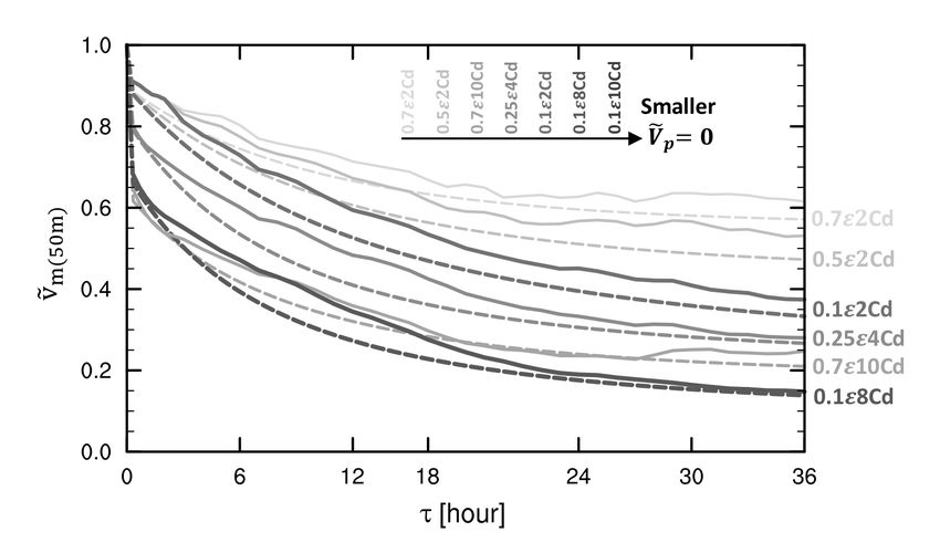
4                 MANUSCRIPT SUBMITTED TO      JOURNAL OF THE ATMOSPHERIC SCIENCES

    When v f = 0, Eq.(10) reduces to                                    TABLE 1. Parameter values of the CTRL simulation.
                                           −1                   Model         Name                             Value
                             Ck vm (0)
             ṽm(th) (τ) =             τ +1              (11)     lh            hor. mixing length               750-m
                                2h                                lin f         asymptotic ver. mixing length    100-m
For this special case, the transient intensity response from      Ck            exchange coef. of enthalpy       0.0015
a given vm (0) depends only on the boundary layer depth           Cd            exchange coef. of momentum       0.0015
scale h. Fig.1b presents examples varying h over a wide           Hdomain       model height                     25-km
                                                                  Ldomain       model radius                     3000-km
range of values, with using vm (0) = 100 ms−1 and v f =
                                                                  Environment   Name                             Value
0. Eq. (11) is the continuous limit of Eq.(10) as v f →
                                                                  TST           surface temperature              300-K
0 and is not singular. Note that setting v f = 0 produces
                                                                  Tt pp         tropopause temperature           200-K
a solution that does not actually reach zero intensity in
                                                                  Qcool         radiative cooling (θ )           1Kday−1
finite time, but rather approaches zero only as τ → ∞; for
                                                                   f            Coriolis Parameter               5 × 10⁻⁵ s−1
realistic timescales, the solution still predicts a normalized
intensity appreciably greater than zero (≈15% after 5 days
in Fig.1).
   According to Eq.(10)-(11), the intrinsic time scale of        requires sophisticated land-surface and boundary layer pa-
intensity decay from the initial condition is determined by      rameterizations (Cosby et al. 1984; Stull 1988; Davis et al.
the boundary layer depth scale h and the steady-state fi-        2008; Nolan et al. 2009; Jin et al. 2010). However, exper-
nal intensity v f , taking Ck as constant, such that a smaller   iments in axisymmetric geometry with a uniform environ-
h leads to a faster decay (Fig.1b). Effects from changes         ment and boundary forcing can reveal the fundamental re-
in the external environment, e.g., surface properties, are       sponses of a mature TC to individual surface roughening
captured in the prediction of v f as discussed below. No-        or drying, as introduced in CC20. Thus, this work extends
tably, the precise definition of h in E12 theory and its re-     the individual forcing experiments of CC20 to simulations
lation to the true boundary layer height, H, is uncertain        where the surface is simultaneously dried and roughened
both theoretically and practically. First and foremost, the      with varying magnitudes of each.
TC boundary layer height H is poorly understood even for            All experiments are performed using the Bryan Cloud
storms over the ocean where the H is approximated by             Model (CM1v19.8) (Bryan and Fritsch 2002) in axisym-
its dynamical or thermodynamical characteristics (Kepert         metric geometry with same setup as Chen and Chavas
2001; Emanuel 1997; Bryan and Rotunno 2009; Zhang                (2020); model parameters are summarized in Table 1. Dis-
et al. 2011; Seidel et al. 2010). Unfortunately, these es-       sipative heating is included. We first run a 200-day base-
timates of boundary layer heights can vary substantially         line experiment to allow a mature storm to reaches a sta-
from one another (Zhang et al. 2011). Moreover, in E12           tistical steady-state, from which we identify the most sta-
theory it is the boundary layer depth specifically within        ble 15-day period. We then define the Control experiment
the deeply-convecting eyewall that is relevant, where air        (CTRL) as the ensemble-mean of five 10-day segments
rapidly rising out of the boundary layer effectively blurs       of the baseline experiment from this stable period whose
the distinction between boundary layer and free tropo-           start times are each one day apart. From each of the five
sphere (Marks et al. 2008; Kepert 2010; Smith and Mont-          CTRL ensemble member start times, we perform idealized
gomery 2010); perhaps for this reason E12 found a value          landfall restart experiments by instantaneously modifying
corresponding to an approximate half-depth of the tropo-         the surface wetness and/or roughness beneath the CTRL
sphere (5km) to perform best. Finally, little is known           TC, which are then averaged into experimental ensembles
about the TC boundary layer height during the landfall           analogous to the CTRL. Surface wetness is modified by
transition. Thus, when evaluating E12 theory, we sim-            decreasing the surface evaporative fraction ε, which re-
ply test a range of values for h and examine the extent          duces the surface latent heat fluxes FLH through the de-
to which variations in the best-fit values of h across exper-    creased surface mixing ratio fluxes Fqv in CM1 (sfcphys.F)
iments align with variations in estimates of the boundary        as
layer.
                                                                                       Fqv = εs10Cq ∆q                      (12)
3. Methodology
                                                                                        FLH = ρLv Fqv                       (13)
   Idealized numerical simulation experiments of landfall
are used to test the theoretical predictions discussed above.
                                                                 where Cq is the exchange coefficients for the surface mois-
                                                                 ture; s10 is the 10-m wind speed; and ∆q is the moisture
a. Simulation setup
                                                                 disequilibrium between the 10-m layer and the sea surface.
   The pronounced spatiotemporal heterogeneity in sur-           Surface roughness is modified by increasing the drag coef-
face properties from storm to storm in real-world landfalls      ficient Cd , which modulates the surface roughness length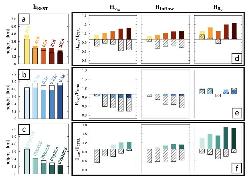
MANUSCRIPT SUBMITTED TO JOURNAL OF THE ATMOSPHERIC SCIENCES 5
Ṽp(Cd ) are labeled in Figure 2. Finally, we generate a spe-
cial set of combined experiments, 0Vp XCd , in which Ṽp is
fully reduced to zero for a range of magnitudes of rough-
ening. Experiments are modeled by setting both surface
sensible and latent heat fluxes to zero while increasing the
roughness by a factor of X. This set of experiments shar-
ing the same Ṽp = 0 and are applied to test the simplified
form of E12 assuming ṽ f = 0 (Eq.(11)).
b. Testing theory against simulations
In each experiment, the simulated storm intensity vm (τ)
is normalized by the time-dependent, quasi-stable CTRL
value, where τ denotes the time since the start of a given
forcing experiment. We primarily focus on the first 36-
F IG . 2. Two-dimensional experimental phase space of surface dry- h evolution, during which ṽm decreases monotonically
ing (decreasing ε moving left to right) and surface roughening (increas-
across all roughening, drying, and combined experiments.
ing Cd moving top to bottom). CTRL is an ocean-like surface with
(Cd , ε) = (0.0015, 1). Values of the potential intensity response Ṽp for In addition, both the near-surface (50m) intensity response
CTRL and individual drying or roughening are listed in parentheses; Ṽp ṽm(50m) and above-BL (2km) intensity response ṽm(2km)
for any combination of forcing is the product of Ṽp for each individual are compared to theoretical predictions. The near-surface
forcing. Experiments testing combined forcings are shaded grey and the wind field is essential for predicting the inland TC hazards,
subset testing the most extreme combinations of each forcing are under-
lined. Experiment set 0Vp XCd , corresponding to the special case where while the above-BL wind field is generally used when
surface heat fluxes are entirely removed (Vp = 0), are shaded green. formulating physically-based theories above the boundary
layer. Over the ocean, ṽm(50m) and ṽm(2km) typically co-
evolve closely (Powell et al. 2003). However, at and after
z0 and in turn the friction velocity u∗ for the surface log- landfall, the response of near-surface winds is expected to
layer in CM1 as deviate from the above-BL winds, particularly in the case
z of roughening, as shown in CC20: there is a very rapid
z0 = ( √κ −1) (14)
e Cd initial response of angular momentum to enhanced fric-
tion near the surface during the first 10 minutes (and espe-
κs1 cially the first 5-6 minutes) that subsequently propagates
u∗ = max , 1.0−6 (15) upward as the vortex decays. In contrast, the response to
za
ln z0 + 1 surface drying initially occurs aloft in the eyewall before
where κ is the von Kármán constant, z = 10m is the refer- propagating into the boundary layer, though this response
ence height, s1 is the total wind speed on the lowest model, is generally slower and smoother in time. Therefore, it
and za is approximately equal to the lowest model level is practically useful to test intensity theories against both
height. Readers are referred to CC20 for full details. near-surface and above-BL winds.
Our experiments are summarized in Fig.2. Surface For E86 theory, we first compare the simulated equilib-
roughening-only experiments (2Cd , 4Cd , 6Cd , 8Cd , 10Cd ) rium intensity against the equilibrium E86 prediction of
and drying-only experiments (0.7ε, 0.5ε, 0.3ε, 0.25ε, Eq.(6). We then compare the full time-dependent simu-
0.1ε) are fully introduced in CC20. The combined ex- lated intensity response against that predicted by assum-
periments are simulated in the same manner but with the ing the total response is the product of the individual re-
surface dried and roughened simultaneously. Our com- sponses, ṽ∗ (τ) (Eq.(8)). For E12 theory, we compare the
bined experiments are designed in a way where individual simulated intensity evolution ṽm (τ) against the E12 pre-
drying and roughening are systematically paired with each diction ṽm(th) (τ) of Eq.(10)-Eq.(11). In these solutions,
other; experiments are named by the corresponding mod- the initial intensity vm (0) = 100.4 ms−1 for 2km wind field
ifications in Cd and ε. We focus on two specific subsets and vm (0) = 90.38 ms−1 for 50m wind field, respectively.
of experiments within this phase space. First, 0.7ε2Cd , The final intensity v f is set as the minimum value of vm in
0.7ε10Cd , 0.1ε2Cd , 0.1ε10Cd are chosen as the repre- each simulation during the evolution. A range of h will be
sentatives for extreme combinations, where each forcing tested in Eq.(10), which will be discussed in the following
takes its highest or lowest non-zero magnitude. Second, subsection. For real-world landfalls, we do not know the
0.25ε4Cd , 0.5ε2Cd , 0.1ε8Cd are chosen to represent cases minimum intensity prior to the inland evolution. Thus, as
where the individual forcings are varied in ways that yield a final step, we compare simulation results against the the-
comparable equilibrium potential intensities; Ṽp(ε) and ory with ṽ f predicted from Ṽp . This final step may be use-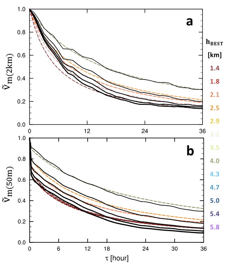
6 MANUSCRIPT SUBMITTED TO JOURNAL OF THE ATMOSPHERIC SCIENCES
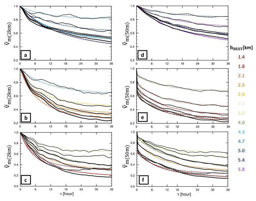
ful for potentially applying the theory to real-world land- roughening experiments, whereas ṽm(2km) responds more
falls. gradually. The magnitude of the deviation of ṽm(50m) from
ṽm(2km) during the first 20 hours increases with increasing
c. The boundary layer depth scale h roughening (Fig.3b), though again both converge to com-
parable values after τ = 20 h. The above behavior is con-
As introduced in Section 2, h is an uncertain bound- sistent with the findings in CC20, where surface roughen-
ary layer height scale both theoretically, as it is assumed ing has a significant and immediate impact on near-surface
to be constant, and in practice, because we do not have intensity while drying first impacts the eyewall aloft. As
a simple means of defining the boundary layer depth par- noted in CC20, Ṽp provides a reasonable prediction for
ticularly during the landfall transition. Thus, we do not the long-term equilibrium intensity response to each indi-
aim to resolve this uncertainty in h in the context of land- vidual forcing; there is a small overshoot in roughening
fall, but rather we simply test what values of h provide the experiments where ṽm reaches a minimum that is less than
best predictions and evaluate to what extent variations in Ṽp at approximately τ = 36 h before increasingly gradu-
h across experiments align with variations in estimates of ally towards Ṽp .
the boundary layer height H. For our combined experiment sets (Fig.3c-d), both sur-
For each simulation, we test a range of constant values face drying and roughening determine the total response
of h from 1.0 to 6.0 km in 0.1 km increments in order to of storm intensity. However, regardless of the relative
identify a best-fit boundary layer depth scale, hBEST . We strength of each forcing, ṽm(50m) always decreases more
define hBEST as the value of h that produces the smallest rapidly than ṽm(2km) due to the surface roughening. Similar
average error throughout the first 36-h evolution for each to the roughening-only experiment, stronger roughening
experiment. We then compare the systematic variation in results in a larger deviation of ṽm(50m) from ṽm(2km) dur-
hBEST against that of three typical estimates of boundary ing the first 20 hours. Overall, the rapid initial response of
layer height H calculated from each simulation. near-surface intensity is controlled by the surface rough-
Since the E12 solution applies within the convecting ening regardless of the surface drying magnitudes. More-
eyewall region, we estimate H using three typical approx- over, similar to the individual forcing experiments, Ṽp pro-
imations and measure the value at the radius of maximum vides a reasonable prediction for the simulated minimum
wind speed (rmax ) at the lowest model level: 1. Hvm is the ṽm in combined experiments used to define the theoretical
height of maximum tangential wind speed (Bryan and Ro- final intensity ṽ f .
tunno 2009); 2. Hin f low is the height where radial wind u
in the eyewall first decreases to 10% of its surface value
(Zhang et al. 2011); and 3. Hθv is defined as the height b. Deconstructing simultaneous drying and roughening
where θv in the eyewall matches its value at the lowest Now we focus on the full time-dependent responses of
model level (Seidel et al. 2010). The 36-h evolution of the combined forcing experiments. As noted above, we
each estimate of H across our simulations is shown in Sup- hypothesized based on traditional potential intensity the-
plementary Figure 1. Considering that H varies in time ory (Eq.(5)-(7)) that the transient response of storm inten-
during the experiment, the averaged value of H during sity to simultaneous drying and roughening can be pre-
τ = 0 − 6 h and τ = 30 − 36 h are each compared to the dicted as the product of their individual responses (Eq.(8)).
hBEST . Thus, we compare the ṽ∗ (τ) to the simulated ṽm (τ) of
near-surface winds for each combined experiment (Fig.4)
4. Results for our experiment set with extreme cases of combined
drying and roughening. Regardless of the magnitude of
a. Near-surface vs. above-BL intensity response
roughening and/or drying, ṽ∗ (τ) follows the simulated
As discussed in Section 3b, the simulated intensity re- ṽm (τ) closely through the initial rapid decay forced by
sponses near the surface (z = 50m) and above the boundary roughening, the weakening stage through 36 hours, and
layer (z = 2km) may differ, and thus we intend to test the the final equilibrium stage. There is a slight low bias in
theory against both. We begin by simply identifying im- ṽ∗ (τ) relative to the ṽm (τ) throughout the primary weak-
portant differences between the intensity responses at each ening stage, especially for strong drying (Fig.4c-d), indi-
level. cating that there is a slight compensation in the response
For drying-only experiments, ṽm(2km) responds to re- to roughening when strong drying is also applied. Overall,
duced ε before ṽm(50m) during the initial ∼ 5 hours though, the full temporal evolution of the normalized re-
(Fig.3a), where stronger drying results in a larger devia- sponses to drying and roughening can indeed be combined
tion between the responses at each level. ṽm(2km) decreases multiplicatively. A very similar result is obtained for the
slightly more rapidly than ṽm(50m) but they eventually con- above-BL intensity as well (not shown).
verge to comparable equilibria. In contrast, for rough- Although E86 theory is formulated for the equilibrium
ening ṽm(50m) responds nearly instantaneously across all intensity, the above results indicate that the implication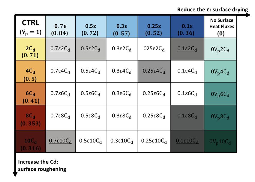
MANUSCRIPT SUBMITTED TO            JOURNAL OF THE ATMOSPHERIC SCIENCES                                                          7

   F IG . 3. Temporal evolution of simulated near-surface (50m, solid curves) and above-BL (2km, dash curves) ṽm , across experiments: (a) surface
drying, (b) surface roughening and (c)-(d) representative combined experiments. Potential intensity response, Ṽp (Eq.(4)-(6)), denoted by horizontal
line. Darker color indicates a smaller Ṽp .

of its underlying physics also extends to the transient re-                    For near-surface winds, E12 theory can capture the tran-
sponse to simultaneous surface drying and roughening.                       sient response of ṽm in drying experiments (Fig.5d) using
This behavior aligns with the notion that periods of in-                    a slightly larger hBEST . For roughening and combined ex-
tensity change represent a non-linear transition of the TC                  periments, though, it misses the very rapid initial decay
system between two equilibrium stable attractors given by                   due to enhanced Cd (Fig.3b-d and Fig.5e-f), which was
the pre-forcing and post-forcing Vp (Kieu and Moon 2016;                    shown in Fig.1 of CC20 to occur within the first 10 min-
Kieu and Wang 2017). Because the distance between at-                       utes. The magnitude of this rapid initial decay depends on
tractors is multiplicative, evidently so too is the trajectory              Cd , as surface roughening immediately acts to rapidly re-
between them.                                                               move momentum near the surface first. To account for this
                                                                            initial response, we propose a simple model for this initial
                                                                            decay of ṽm(50m) that may be derived from the tangential
c. Testing theory for transient intensity response                          momentum equation in a 1D slab boundary layer with a
   We next test the extent to which E12 theory (Eq.(10)                     depth of h∗ , given by
and Eq.(11)) can predict the intensity evolution, taking as
input ṽ f and a best-fit value of hBEST from each simula-                                                dv
tion. The subsequent subsection compares the systematic                                              h∗      = −Cd |v| v                       (16)
                                                                                                          dt
variation in hBEST against that of the estimated H in each
set of experiments.
   We begin by focusing on the above-BL intensity. The                      Taking |v| ≈ v, this equation may be integrated and then
E12-based solution (Eq. (10)) can reasonably capture the                    normalized by an initial intensity vm (0) to yield
overall transient intensity response across all roughening,
drying, and combined experiments (Fig.5a-c). For drying-
                                                                                                                Cd vm (0)
                                                                                                                                 −1
only experiments (Fig.5a), the theory initially (τ < 5 h)                                   ṽm(th) (τ) =                 τ +1                 (17)
                                                                                                                   h∗
underestimates ṽm(2km) (Fig.3a). hBEST in drying experi-
ments takes a value around 5 km and shows little system-
atic variations with increased drying magnitude (Fig.5a).                   Curiously, Eq.(17) is mathematically identical to the E12
In contrast, hBEST decreases with increased surface rough-                  solution with v f = 0 (Eq.(11)) except with Ck replaced by
ening, from 4.3 km to 2.1 km (Fig.5b). In the following                     2Cd , a topic we return to in the summary section.
subsection, we compare this variation in hBEST to that of                     We may combine Eq.(17) for the first 10-min evolution
multiple estimates of H.                                                    with Eq.(10) to model the complete near-surface intensity
8 MANUSCRIPT SUBMITTED TO JOURNAL OF THE ATMOSPHERIC SCIENCES
F IG . 4. Temporal evolution of simulated ṽm (τ) for four representative combined experiments (solid purple) and their associated individual
forcing experiments (solid blue for drying, solid red for roughening), with prediction ṽ∗ (τ) (dash purple; Eq.(8)) defined as the product of the
individual forcing responses. Horizontal line denotes Ṽp , colored by experiment.
response to surface roughening: solution; the 10-minute period is short enough that the dif-
ference is likely not of practical significance. Thereafter,
−1
Cd vm (0)
τ + 1 τ ≤ 10 min we estimate hBEST for each simulation in the same manner
h ∗
ṽm(th) (τ) = Ck v f
as before.
ṽ f coth ( 2h τ + tanh−1 (ṽ∗f ))
τ > 10 min The comparison of model against simulations is shown
(18) in Fig.5e-f. Eq.(18) can capture the simulated near-surface
vf
where ṽ∗f = vm(th) (10 min) since vm(th) now decreases from transient intensity response ṽm (τ) across roughening and
a new initial intensity vm(th) (10 min) calculated from the combined experiments. The values of hBEST for the pre-
first equation. For the τ ≤ 10 min solution, we find that diction of ṽm(50m) are similar to those obtained for the
the rapid decay by τ = 10 min across all roughening ex- above-BL case but slightly smaller in magnitude (Fig.5b,e
periments can be captured by setting h∗ = 1.78 km con- and c,f).
stant, which yields a constant decay rate during the period Similar behavior associated with roughening is found in
τ = 0 − 10 min. In reality, the decay rate is very large experiments for the special case v f = 0 (Fig.6). Thus, we
in the first minute and monotonically decreases through again propose a two-stage model for ṽm(50m) given by
the 10 minute period. This time-varying decay rate can −1
Cd vm (0)
be reproduced by allowing h∗ to increase with time from
h∗ τ + 1 τ ≤ 10 min
an initial very small value, which aligns with the physi- ṽm(th) (τ) = −1
Ck vm (0) vm (0)
cal response to roughening that may be thought of as the 2h τ + vm(th) (10 min)
τ > 10 min
formation of a new internal boundary layer that begins at (19)
the surface and rapidly expands upward. Here though we The comparison of model against simulations is shown in
employ a constant h∗ in order to retain a simple analytic Fig.6, where hBEST exhibits a decreasing trend with en-MANUSCRIPT SUBMITTED TO JOURNAL OF THE ATMOSPHERIC SCIENCES 9
F IG . 5. (a-c) Temporal evolution of the simulated above-BL (2km) winds ṽm (τ) (solid black) and theoretical prediction ṽm(th) (τ) (dash colored;
Eq.(10)) for (a) drying, (b) roughening and (c) combined experiments. ṽm(th) (τ) is colored by the value of best-fit value of h, hBEST . (d-f) are same
as (a-c) but for the near-surface (50m) wind, in which (e-f) are the predictions from Eq.(18) to account for the initial rapid decay due to roughening.
hanced surface roughening, similar to that found in the tion is likely not instantaneous, though we have modeled
pure roughening experiments. it as so here for simplicity. The details of this adjustment
Note that multiplying both sides of (17) by v yields process warrant more in-depth investigation that is left for
a budget equation for kinetic energy given by h d(KE) dt = future work.
3 1 2
−Cd v , where KE = 2 v and the RHS is the expression
for surface frictional dissipation of kinetic energy that is 1) C OMPARING THE VARIATION OF hBEST AND ESTI -
standard in TC theory (Bister and Emanuel 1998; Tang MATES OF H
and Emanuel 2010; Chavas 2017)1 . Physically, then, the
solution for the initial roughening response represents the We next compare the variations of hBEST from our simu-
intensity response to the dominant sink of kinetic energy lations to that of three common estimates of the boundary
in the absence of the dominant compensating thermody- layer height: Hvm , Hin f low , and Hθv . We compare trends
namic source of kinetic energy from surface heat fluxes for both the initial response (0-6h) and the equilibrium re-
for a tropical cyclone. After this initial response, the so- sponse (30-36h) (Fig.7d-f). As noted above, hBEST was
lution follows a solution that accounts for both source and found to decrease with increased roughening (Fig.7a) but
sink as encoded in E12 theory. The interpretation is that remain relatively constant for increased drying (Fig.7b).
there exists a brief initial period where surface roughen- Moreover, hBEST values are quite similar when estimated
ing directly modifies the near-surface air in a manner that from the above-BL vs. near-surface responses (Fig.7a-c),
is thermodynamically independent of the rest of the vor- and hence this discussion is not dependent on the choice
tex. Thereafter, the vortex has adjusted and weakening of level for defining hBEST .
proceeds according to processes governed by the full TC To show the variation of estimates of H in different
system, analogous to that of drying. In reality this transi- sets of experiments, we normalize each H by its corre-
H
sponding value in the CTRL experiment as HCTexpRL (Fig.7d-
f), where each estimate of H in the CTRL experiment is
1 Note: the KE budget equation may be expressed as h d(KE)
dt = quasi-stable (Supplementary Fig.1). We focus first on the
−2Cd |v|(KE). Hence, 2Cd represents the surface exchange coefficient
of kinetic energy over a static surface.10 MANUSCRIPT SUBMITTED TO JOURNAL OF THE ATMOSPHERIC SCIENCES
the pure drying experiments where hBEST remains constant
with enhanced drying. The systematic variation in hBEST
disagrees with both the early and the slow response of all
three estimates of H (Fig.7 c,f).
Note that for the combined experiments, there is no
clear evidence to link the decreasing trend in hBEST
(Fig.5c,f) to the change in each individual forcing. Thus,
we elect not to speculate on the details of hBEST and H
for the combined experiments; instead, we explore a more
practical theoretical prediction for combined forcing cases
that applies hBEST to drying and roughening experiments
individually as shown in the next section.
The disagreement in the systematic trends both among
estimates of H and between those estimates H and hBEST
motivates the need for more detailed studies on the TC
boundary layer during and after the landfall in future work.
In terms of E12 theory, though the solution can reproduce
the decay evolution, it also likely oversimplifies the TC
boundary layer, where a constant h cannot fully capture
the time- and the radially-varying response of boundary
layer height to landfall-like surface forcing. In terms of
boundary layer theory, the optimal definition of boundary
F IG . 6. Temporal evolution of simulated intensity response and the- layer depth is itself uncertain. Meanwhile, without a com-
oretical prediction for the experiment set 0Vp XCd : (a) above-BL 2km prehensive understanding of the TC boundary layer during
winds (Eq.(11)) and (b) near-surface 50m winds (Eq.(19)). E12-based the landfall, it is unclear if one particular definition of H,
prediction is colored by the value of hBEST for corresponding experi- if any, might be most appropriate for E12 theory within
ment.
the eyewall. Therefore, having a better estimation of h in
the E12 solution and an improved understanding of bound-
ary layer evolution during the landfall would help explain
responses to pure roughening or pure drying (Fig.7, top
the differences in systematic variations between h and es-
two rows). During 0-6h, all three estimates of H slightly
timates of H.
increase with enhanced roughening and are approximately
constant with enhanced drying (Fig.7d-f, color). By 30-
36h, H decreases with enhanced roughening and enhanced d. Predicting the intensity response combining equilib-
drying for Hvm and Hin f low , while Hθv remains relatively rium and transient theory
constant for each (Fig.7d-f, shaded). We may combine all theoretical findings presented
Overall, there is no single estimated H whose sys- above to predict the near-surface intensity response to
tematic variation matches that of hBEST (Fig.7). For idealized landfalls for experiments combining drying and
roughening-only experiments, the initial response of all roughening. This represents the most complex of our ex-
three estimates of H with enhanced roughening is opposite perimental outcomes. We begin from the result of Eq.(8)
to that of hBEST (Fig.7a,d), though the slow response of and predict the intensity response to simultaneous surface
each H for two of the estimates does show a decrease with drying and roughening as the product of their individual
enhanced roughening (Fig.7d, shaded). For drying-only predicted intensity responses:
experiments, the initial response of H is either constant or
very slowly decreasing with enhanced drying (Fig.7b,e), ∗
ṽth(Cd ε) ≈ ṽth = ṽth(Cd ) ṽth(ε) (20)
similar to hBEST . However, the slow response of Hvm and
Hin f low decreases with enhanced drying in contrast to the where ṽth(ε) is generated by Eq.(10) and ṽth(Cd ) is gener-
nearly constant hBEST , while the slow response of Hθv is ated by Eq.(18). When applying the transient solution for
again relatively constant (Fig.7e, shaded). each individual forcing component, we use the previously-
Finally, for 0Vp XCd experiments (Fig.6), hBEST exhibits identified hBEST from Fig.7a-b and predict the ṽ f using
a similar systematic response to enhanced surface rough- Ṽp given by Eq.(4)-(5). In principle, an empirical model
ening as the pure roughening experiments (Fig.7 a,c). for hBEST for each individual forcing could be generated
Turning off all heat fluxes does not significantly alter the from our data since hBEST is approximately constant with
variation of hBEST with roughening relative to the pure- enhanced drying and monotonically decreasing with en-
roughening experiments; this behavior is also similar to hanced roughening. But given the uncertainties in hBESTMANUSCRIPT SUBMITTED TO JOURNAL OF THE ATMOSPHERIC SCIENCES 11
F IG . 7. Comparison of hBEST (a-c) and the systematic variation of three estimates of boundary layer depth H (d-f) for each set of surface
roughening, surface drying, and 0Vp XCd experiments. For (a-c), hBEST is shown for above-BL (color) and near-surface (box) intensity predictions.
H
For (d-f), H exp is shown for the early period (τ = 0 − 6h; color) and later period (τ = 30 − 36h; hatched box). The CTRL values of Hvm , Hin f low ,
CT RL
and Hθv are 0.95km, 1.56km, and 0.67km, respectively.
as a true physical parameter, we elect not to take such a
step here.
The results are shown in Fig.8. Overall, our analytic
theory performs well in capturing the first-order response
across experiments, particularly given the relative simplic-
ity of the method. There is a slight low bias in ṽth(Cd ε)
(i.e., too strong of a response) across all the predictions
relative to the simulations, a reflection of the slight com-
pensation found in the assumption that the combined re-
sponse may be modeled as the product of the individual
responses in Fig.4. Therefore, knowing how each sur-
face forcing is changed after landfall provides a theoretical
time-dependent intensity response prediction when given
estimates of Ṽp and hBEST for any combination of uniform F IG . 8. Temporal evolution of simulated near-surface intensity re-
sponse for combined forcing experiments (solid) and the correspond-
surface forcing. This offers an avenue to link our theoreti- ing prediction combining the equilibrium and transient theory (dash;
cal understanding to real-world landfalls. Eq.(20)), with ṽ f = Ṽp and setting h equal to the values of hBEST for
the individual predicted responses to drying (Eq.(10)) and roughening
e. Comparison with existing empirical decay model (Eq.(18)).
Finally, as a first step toward linking theory and real-
world landfalls, we provide a simple comparison of our
theoretical model with the prevailing empirical model for
inland decay. The model was first introduced by DeMaria where storm landfall intensity V0 decays to a background
and Kaplan (1995) and most recently applied to historical intensity Vb with a constant exponential decay rate α.
observations by Jing and Lin (2019) as Jing and Lin (2019) estimated Vb = 18.82 kt (9.7 ms−1 )
and α = 0.049 h−1 using the historical Atlantic hurricane
V (t) = Vb + (V0 −Vb )e−αt (21) database.12 MANUSCRIPT SUBMITTED TO JOURNAL OF THE ATMOSPHERIC SCIENCES
F IG . 9. Comparison between the theoretical intensity prediction for v f = 0 (Eq.(11)) against the prevailing empirical exponential decay model
prediction from Jing and Lin (2019) (Eq.(21)) for a range of initial intensities ([100, 75, 60, 50, 36, 23] ms−1 ). For the theoretical prediction,
h=5km.
Comparisons between theory and Eq.(21) predictions of a mature tropical cyclone to surface drying, roughen-
are shown in Fig.9, for V0 from 100 ms−1 to 23 ms−1 sim- ing, and their combination. This work builds off of the
ilar to Jing and Lin (2019) (their Fig.3). Given that TCs in mechanistic study of Chen and Chavas (2020) that ana-
nature eventually dissipate (and typically do so rapidly), lyzed the responses of a mature tropical cyclone to these
we choose the theoretical equation with v f = 0 (Eq.(11)); surface forcings applied individually. Key findings are as
this is also by far the simplest choice as no final intensity follows:
information is required. We set h = 5km constant. Eq.(11)
• The transient response of storm intensity to any com-
compares well against the empirical prediction for inland
bination of surface drying and roughening is well-
intensity decay, capturing the first-order structure of the
captured as the product of the response to each forc-
characteristic response found in real-world storms. The
ing individually (Eq.(8)). That is, the time-dependent
comparison is poorer for weaker cases (Fig.9e-f), though
intensity evolution in response to a land-like sur-
uncertainties in intensity estimates are also likely highest
face can be understood and predicted via decon-
for such weak storms. Note that the structure of the em-
structed physical processes caused by individual sur-
pirical model is constrained strongly by the assumption face roughening and drying. Surface roughening im-
of an exponential model, so differences beyond the gross poses a strong and rapid initial response and hence
structure should not be overinterpreted. Ultimately, the dominates decay within the first few hours regardless
consistency with the empirical model provides additional of the magnitude of drying.
evidence that the physical model may indeed be applica-
ble to the real world. Hence, it may help us to develop a • The equilibrium response of storm intensity to si-
physically-based understanding of the evolution of the TC multaneous surface drying and roughening is well-
after landfall. predicted by traditional potential intensity theory
(Eq.(6)).
5. Summary • The transient response of storm intensity to drying
and roughening can be predicted by the intensifica-
This work tests the extent to which equilibrium and tion theory of Emanuel (2012), which has been gen-
transient tropical cyclone intensity theory, the latter refor- eralized to apply to weakening in this work (Eq.(10)).
mulated here to apply to inland intensity decay, can predict This theory predicts an intensity decay to a final,
the simulated equilibrium and transient intensity response weaker equilibrium that can be estimated by Eq.(6).MANUSCRIPT SUBMITTED TO JOURNAL OF THE ATMOSPHERIC SCIENCES 13
The intensity prediction also depends on the bound- surface forcings in an idealized setting provides a founda-
ary layer depth scale h, whose best-fit values are com- tion for understanding TC landfall in nature. In this vein,
parable to the value used in E12. Systematic trends of our results suggest that the TC landfall process could plau-
h to surface forcings do not clearly match commonly- sibly be deconstructed into transient responses to individ-
defined TC boundary layer height. ual surface and/or environmental forcings as encoded in
our existing theories. One implication of this work is the
• An additional modification is required to model the potential to predict how post-landfall intensity decay may
near-surface (50m) response specifically for surface change in a changing climate if we know how each sur-
roughening, which induces a rapid initial decay for face forcing will change in the future (Zeng and Zhang
near-surface intensity during the first 10 minutes. 2020). Theoretical solutions presented in this work could
The magnitude of this initial rapid response increases also benefit current risk models for hazard prediction.
with enhanced roughening and can be modeled an- In terms of theory, future work may seek to test the the-
alytically as a pure frictional spin-down (Eq.(17)- ory against simulations in three-dimensional and/or cou-
(18)). pled models that include additional complexities. That
said, several questions pertinent to axisymmetric geom-
• The above findings about the transient and equilib-
etry remain open here: do changes in surface sensible heat
rium responses can be applied together to generate
fluxes significantly alter the response to surface drying?
a theoretical prediction for the time-dependent in-
How might changes in Ck , whose variation after landfall
tensity response to any combination of simultaneous
is not known, alter the results? How should one optimally
surface drying and roughening (Eq.(20)). This pre-
define TC boundary layer height for the convective eye-
diction compares reasonably well against simulation
wall region where boundary layer air rises rapidly into up-
experiments with both surface forcings.
drafts, both in general and in the context of the transition
• In the special case where the final equilibrium inten- from ocean to land? How best can this be used to approx-
sity is taken to be zero, the E12 solution reduces to a imate the boundary layer depth scale h in the theoretical
simpler analytic form that depends only on initial in- solution?
tensity and boundary layer depth (Eq.(11)). This so- Notably, the solution for pure frictional spin-down
lution is found to compare well against experiments (Eq.(17)) and the E12 solution for zero final intensity
with surface fluxes turned off for a range of magni- (Eq.(11)) have an identical mathematical form, with the
tudes of surface roughening. It also compares well lone difference being trading the parameter Ck for 2Cd .
with the prevailing empirical model for landfall de- These are simply the exchange coefficients for the dom-
cay (Eq.(21)) across a range of initial intensities. inant kinetic energy source (enthalpy fluxes) and sink
(frictional dissipation) for the TC, respectively. Phys-
Although existing intensity theories are formulated for ically, we interpreted these two solutions as found in
the tropical cyclone over the ocean, the above findings our work as a transition from a rapid response governed
suggest that those underlying physics may also be valid in by pure frictional spin-down to a response governed by
the post-landfall storm evolution. Note that we have not the reintroduction of the counterbalancing thermodynamic
systematically tested the underlying assumptions of the source of energy for the tropical cyclone as encoded in
theory but have focused on testing the performance of the- Emanuel (2012) theory (and similarly in traditional time-
ories for predicting the response to idealized landfalls. The dependent Carnot-based theory). More generally, though,
principal result is that for an idealized landfall, one can why should the large difference in the underlying physics
generate a reasonable prediction for the time-dependent of these two regimes manifest itself mathematically as a
intensity evolution if the inland surface properties along simple switch in exchange coefficients? This is curious.
the TC track are known. Finally, future work may seek to test these theoretical
Landfall in the real world is certainly much more predictions against observations accounting for variations
complicated. The real world has substantial horizon- in surface properties. Here we showed that our physically-
tal variability in surface properties compared to the sim- based model appears at least broadly consistent with the
plified idealized landfalls where only the surface rough- prevailing empirical exponential decay model, suggesting
ness and wetness beneath the storm are instantaneously that our model may provide an avenue for explaining vari-
and uniformly modified. Additional environmental vari- ability in decay rates both spatially and temporally, includ-
ability during the transition, including heterogeneity in ing across climate states. For example, theory may be use-
surface temperature and moisture, environmental stratifi- ful to understand how surface properties facilitate those
cation, topography, land-atmosphere feedbacks, vertical rare TCs that do not weaken after the landfall (Evans et al.
wind shear, and translation speed, is excluded in these 2011; Andersen and Shepherd 2013). This would help us
idealized simulations. Therefore, a theoretical prediction link physical understanding to real-world landfalls, which
for the first-order intensity response to major post-landfall is important for improving the modeling of inland hazards.14 MANUSCRIPT SUBMITTED TO JOURNAL OF THE ATMOSPHERIC SCIENCES
Acknowledgments. The authors thank for all conversa- References
tions and advice from Frank Marks, Jun Zhang, Xiaomin Andersen, T., and J. M. Shepherd, 2013: A global spatiotemporal anal-
Chen on the hurricane boundary layer. The authors were ysis of inland tropical cyclone maintenance or intensification. Int. J.
supported by NSF grants 1826161 and 1945113. We also Climatol., 34, 391–402.
thank for all feedbacks and conversations related to this re-
Bhowmik, S. K. R., S. D. Kotal, and S. R. Kalsi, 2005: An empirical
search during 101th AGU and AMS annual fall meetings. model for predicting the decay of tropical cyclone wind speed after
landfall over the indian region. J. Appl. Meteor., 44(1), 179–185.
Bister, M., and K. E. Emanuel, 1998: Dissipative heating and hurricane
APPENDIX intensity. Meteor. Atmos. Phys., 65, 233–240.
The E12-based decay solution is derived from Eq.17 of Bryan, G., and R. Rotunno, 2009: The maximum intensity of tropical
cyclones in axisymmetric numerical model simulations. Mon. Wea.
Emanuel (2012), given by
Rev., 137, 1170–1789.
∂ vm Ck Bryan, G. H., and J. M. Fritsch, 2002: A benchmark simulation for
= (v f 2 − vm 2 ) (A1) moist nonhydrostatic numerical models. Mon. Wea. Rev., 130, 2918–
∂τ 2h
2928.
where vm is the initial intensity (maximum tangential wind Chavas, D. R., 2017: A simple derivation of tropical cyclone ventilation
speed) and v f is defined as the theoretical steady-state theory and its application to capped surface entropy fluxes. J. Atmos.
maximum intensity. However, v f need not be larger than Sci., 74(0), 2989–2996.
the current intensity but rather may be generalized to any
Chen, J., and D. R. Chavas, 2020: The transient responses of an ax-
final quasi-steady intensity, larger or smaller. Integrating isymmetric tropical cyclone to instantaneous surface roughening and
Eq.A1 yields: drying. J. Atmos. Sci., 77(8), 2807–2834.
1 Ck Cosby, B. J., G. Hornberger, R.B.Clapp, and T. Ginn, 1984: A statis-
Z Z
dvm = dτ (A2) tical exploration of the relationships of soil moisture characteristics
v f 2 − vm 2 2h to the physical properties of soils. Water Resources Research, 20(6),
682–690.
ln vm + v f − ln vm − v f Ck
= τ +C (A3) Davis, C. A., and Coauthors, 2008: Prediction of landfalling hurricanes
2v f 2h with the advanced hurricane wrf model. Mon. Wea. Rev., 112, 1990–
2005.
vm + v f Ck v f
= e(2 2h τ+C) (A4) DeMaria, M., and J. Kaplan, 1994: Sea surface temperature and
vm − v f the maximum intensity of atlantic tropical cyclones. J. Climate, 7,
1324–1334.
Ramsay et al. (2020) showed that for intensification where
DeMaria, M., and J. Kaplan, 1995: A simple empirical model for pre-
vm < v f , the solution is dicting the decay of tropical cyclone winds after landfall. J. Appl.
Meteor., 34, 2499–2512.
C v vf
(2 k2h f τ+coth−1 ( v (0) ))
e
m −1 DeMaria, M., J. A. Knaff, and J. Kaplan, 2006: On the decay of
vm(th) (τ) = v f C v vf tropical cyclone winds crossing narrow landmasses. J. Appl. Me-
(2 k2h f τ+coth−1 ( v (0) ))
e +1m (A5) teor.Climatol., 45, 491–499.
Ck v f vf
= v f tanh ( τ + coth−1 ( )) DeMaria, M., M. Mainelli, L. K. Shay, J. A. Knaff, and J. Kaplan, 2005:
2h vm (0) Further improvements to the statistical hurricane intensity prediction
scheme (ships). Wea. Forecasting, 20, 531–543.
Eq.A5 reduces to Eq.19 of Emanuel (2012) when vm (τ =
v Emanuel, K., S. Ravela, E. Vivant, and C. Risi, 2006: A statistical deter-
0) = 0, for which coth−1 ( 0f ) = 0. ministic approach to hurricane risk assessment. Bull. Amer. Meteor.
Alternatively, for decay where v f < vm , the solution is Soc., 87(3), 299–314.
C v vf Emanuel, K. A., 1986: An air-sea interaction theory for tropical cy-
(2 k2h f τ+tanh−1 ( v (0) ))
+1 clones. part i: Steady-state maintenance. J. Atmos. Sci., 43, 585–605.
e
m
vm(th) (τ) = v f C v vf
(2 k2h f τ+tanh−1 ( v (0) )) Emanuel, K. A., 1997: Some aspects of hurricane innercore dynamics
e −1 m (A6)
and energetics. J. Atmos. Sci., 54, 1014–1026.
Ck v f −1 vf
= v f coth ( τ + tanh ( )) Emanuel, K. A., 2012: Self-stratification of tropical cyclone outflow:
2h vm (0)
Part ii: Implications for storm intensification. J. Atmos. Sci., 69,
988–996.
Eq.A6 may be normalized by vm (0) to define the intensity
response relative to the initial intensity. Emanuel, K. A., 2018: Corrigendum. J. Atmos. Sci., 75(6), 2155–2156.You can also read